A Polygonal Terrain on Southern Martian Polar Cap: Implications for Its Formation Mechanism

Abstract

Polygonal terrains on a Martian southern polar cap have been observed in high-resolution images by the Mars Orbiter Camera. However, their formation mechanism is enigmatic due to the lack of constraints from their geometric and physical properties. Here we proposed a series of recognition procedures on an image of polygonal terrain located at Australe Scopuli taken by a High-Resolution Imaging Science Experiment. Then, we quantitatively analyzed the areas, orientations and polygon edge densities (~0.10 to ~0.06 in different subregions) of the polygonal terrain. Based on the recognition results, three elevation-related subregions can be distinguished according to the distributions of polygon size and orientation. The two side subregions distribute relatively small and relatively large polygons, respectively. The middle subregion can be regarded as an intermediate zone along the slope (~1°). The intermediate zone is squeezed by the surrounding polygons, indicating a possible uplift or subsidence on previous or present Mars. This paper found a possible formation mechanism of the polygonal terrain located at the south pole of Mars, suggesting that polar-ice-cap polygons are formed during the process of lateral sliding gravity-driven plastic creep and the deformation of ice, with the polygon boundaries being reshaped during the alignment at high slopes and partially compressed at low slopes. These properties and possible formation mechanisms could provide more constraints on understanding ancient and/or present climates on Mars.

1. Introduction

Polygonal terrains are found on the Earth’s cold regions and other solar planets [1,2,3]. On the surface of Mars, polygonal terrains are widespread in mid-high latitudes [4,5,6,7,8,9]. Possible mechanisms of Martian polygonal terrain formation include contraction from desiccation of wet sediment, contraction from cooling lava, and freeze-thaw cycles [10,11,12]. The southern polar cap of Mars is mainly composed of perennial thin CO₂-ice deposits [13] overlying a thick water–ice layer [14,15], with seasonal condensation and sublimation on the top [16,17]. Investigating these polygonal terrains’ characteristics and possible formation mechanisms could provide more constraints on understanding ancient and/or present climates on Mars.

The main geometric properties of the polygonal terrain include diameter, orientation, and polygon edge density. Polygon diameters are widely distributed from dm- to km-scale [1,18]. The difference in the polygon diameters is considered to be related to multiple mechanisms [11,19,20]. Possible mechanisms for different polygonal terrain orientations include the polygonal terrain’s slope and a possible anisotropic stress field [21]. The crack properties are related to the effect caused by temperature changes and the initial water or salt content [22,23,24,25]. Although some south-pole polygonal terrains are observed in high-resolution images by the Mars Orbiter Camera [26], the formation mechanism of the polygonal terrain on the Martian southern polar cap has been given limited attention in the literature [27,28]. In addition, the geometric and physical properties of Martian polygonal terrains lack systemic quantitative evaluation.

Here, we processed an image from the High-Resolution Imaging Science Experiment (HiRISE) [29] and detected the boundaries of polygonal terrains at Australe Scopuli on the southern polar cap of Mars. Then, the statistical information of its area, orientation, and polygon edge density were quantitatively analyzed. Finally, we built up some constraints on the formation mechanism of these polygonal terrains.

2. Region of Study and the Methods of the Recognition for Polygon Properties

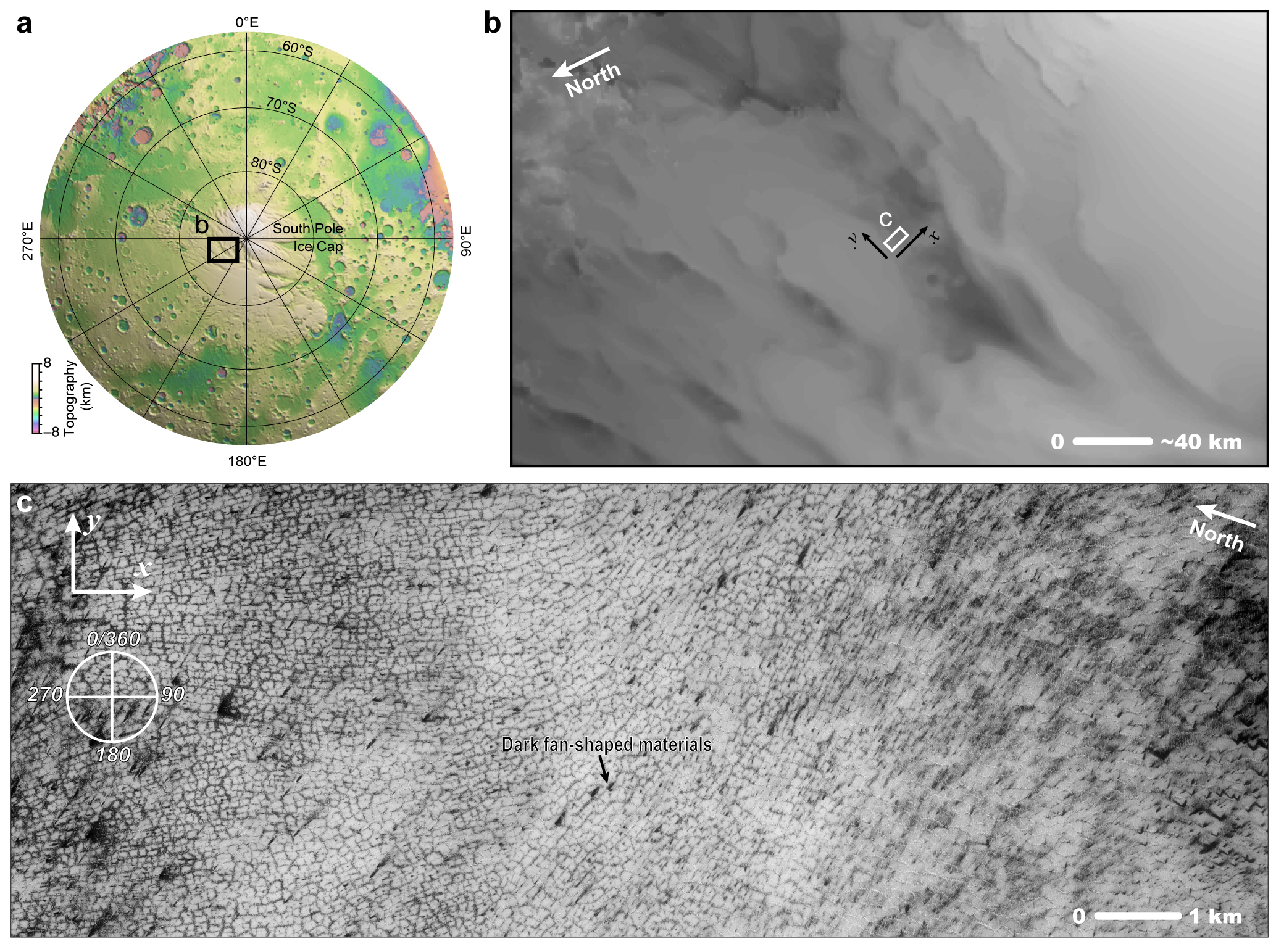
2.1. Region of Study

The study region is located at Australe Scopuli on the south pole of Mars (85.039°S, 259.048°E, Figure 1a,b). Figure 1c presents the picture obtained by HiRISE, showing a region with a polygonal terrain distributed on the surface. The polygons are half-covered by dark fan-shaped materials made up of small particles and distributed by the wind from a particular direction [16]. The size and elongation orientation of the polygons vary, with locations along the HiRISE image (Figure 1c).

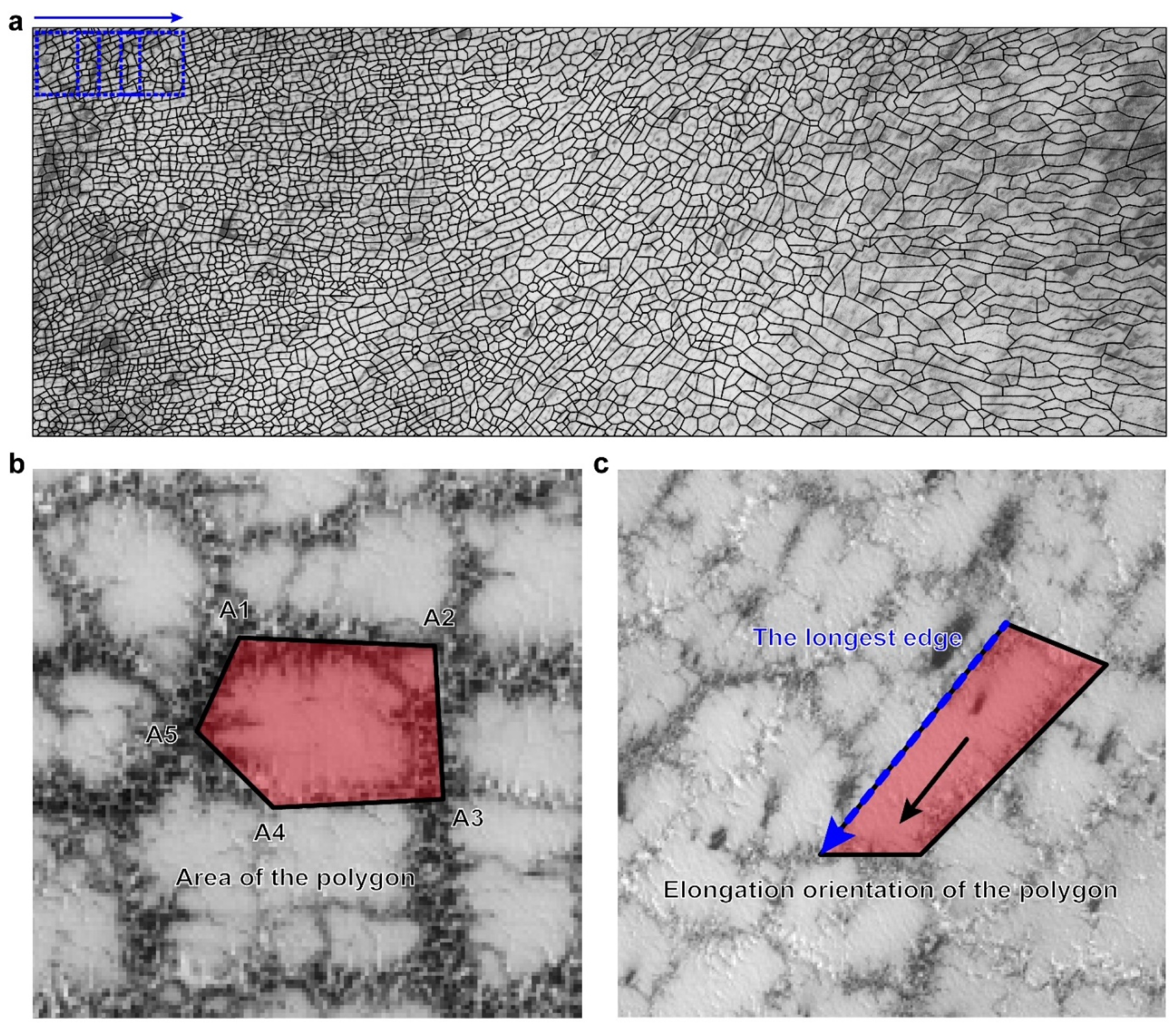
2.2. Recognition Process of the Polygons: Area, Orientation, and Polygon Edge Density

The map was vectorized as polygons (Figure 2a), typically pentagons and hexagons. The edges between the polygonal terrains are represented with lines of the vectorized polygons. The points (A_i) of the polygon with n edges can be marked (Figure 2b) with locations A₁ (x₁, y₁), A₂ (x₂, y₂), …, A_n (x_n, y_n). The area of an individual polygon (S) can be calculated as

$$S=\frac{1}{2}|{\sum }_{i=1}^n(x_i{y}_{i+1}-x_{i+1}{y}_i)|,$$

(1)

where x_{n + 1} = x₁, and y_{n + 1} = y₁.

Figure 2. The procedures of image processing for the polygons. (a) The recognition result of the individual polygons. A series of regions are marked with a dashed box to illustrate the definition of polygon edge density. Two partially enlarged views are presented in (b,c) for the illustration of the recognition process of polygons. (b) The recognition of the polygons. The area of a polygon is shaded. The points of the polygon are marked as A_i (i = 1, 2, 3, …). (c) Elongation orientation of the polygon (black arrow) is defined as the orientation of the longest edge (dashed arrow).

Figure 2. The procedures of image processing for the polygons. (a) The recognition result of the individual polygons. A series of regions are marked with a dashed box to illustrate the definition of polygon edge density. Two partially enlarged views are presented in (b,c) for the illustration of the recognition process of polygons. (b) The recognition of the polygons. The area of a polygon is shaded. The points of the polygon are marked as A_i (i = 1, 2, 3, …). (c) Elongation orientation of the polygon (black arrow) is defined as the orientation of the longest edge (dashed arrow).

The elongation orientation of the polygons shows a spatial variation, especially in the middle subregions (Figure 2a). Here, we evaluated this variation by defining the elongation orientation of an individual polygon along its long edges (Figure 2c). Note that north is defined as zero degrees, clockwise is positive, and the range of the elongation orientation is 0°~180°. The entire image with polygonal terrains can be divided into three subregions, according to the similarity of size, shape and elongation orientation (Figure 3).

Polygon edge density is a key parameter for the geometric property of polygonal terrain. In each local region of the image (Figure 2a), all the pixels can be further divided into the edge and non-edge pixel points. Given that the edge widths of all the polygons are basically the same, we define polygon edge density (unitless) as the ratio of the number of edge pixel points and the number of all pixel points in this local region.

3. Recognition Results

3.1. Areal Distribution of the Polygons

Figure 3a shows the recognized polygons and the areal distribution. The largest and smallest areas of the recognized polygons are ~2500 m² and ~20 m², respectively. The areas of the polygons are small on the –x subregion and large on the +x subregion, with a transition zone in the middle (Figure 3a). Partial enlargements for three representative polygons in the three subregions are shown in Figure 3b–d. According to the areal distribution of the recognized polygons in the three subregions (Figure 3e–g), the –x, middle and +x subregions have individual polygon areas of ~121.6 m², ~218.6 m², and ~574.9 m², respectively.

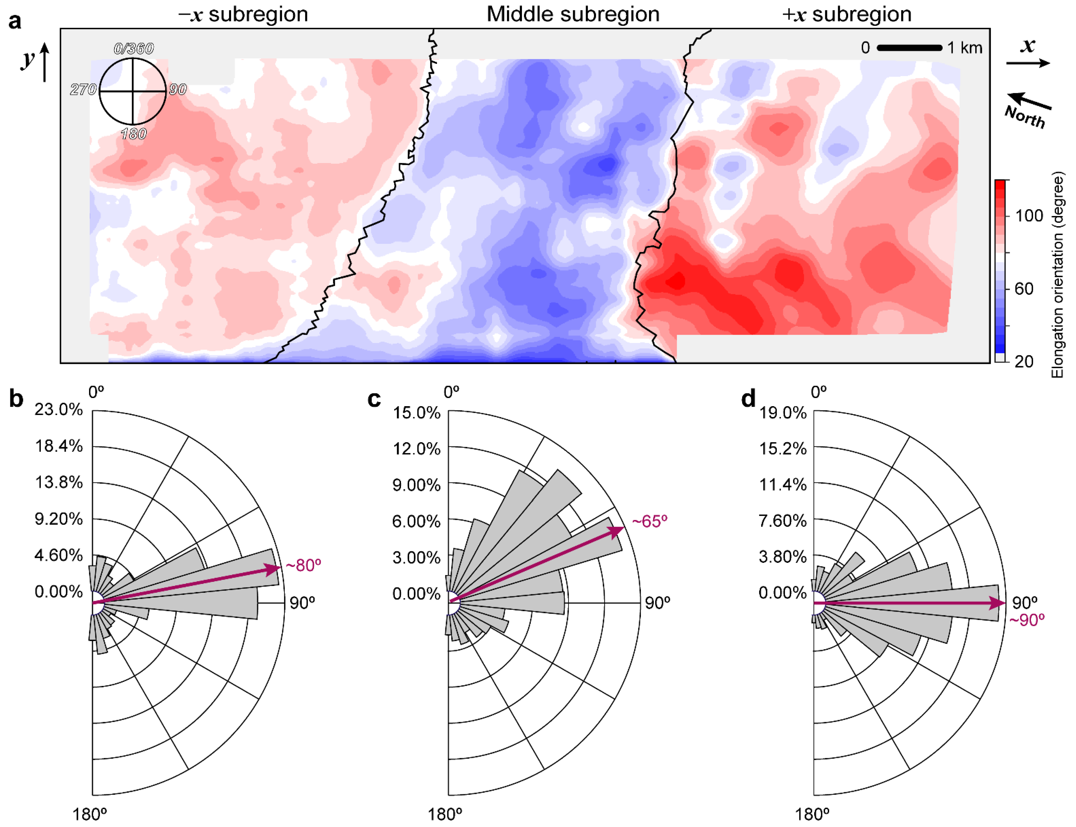
3.2. Distribution of Elongation Orientation of the Polygons

Figure 4a presents the smoothed distribution of elongation orientation of the recognized polygons, showing three subregions consistent with that in Figure 3a. The dominant orientations of the –x, middle and +x subregions are ~80°, ~65°, and ~90°, respectively (Figure 4b–d). It is important to note that the middle subregion has an anomalous orientation, while the –x and +x subregions have nearly east–west orientations (~80° and ~90°, respectively), indicating that the middle subregion might have experienced different deformation than the surrounding regions.

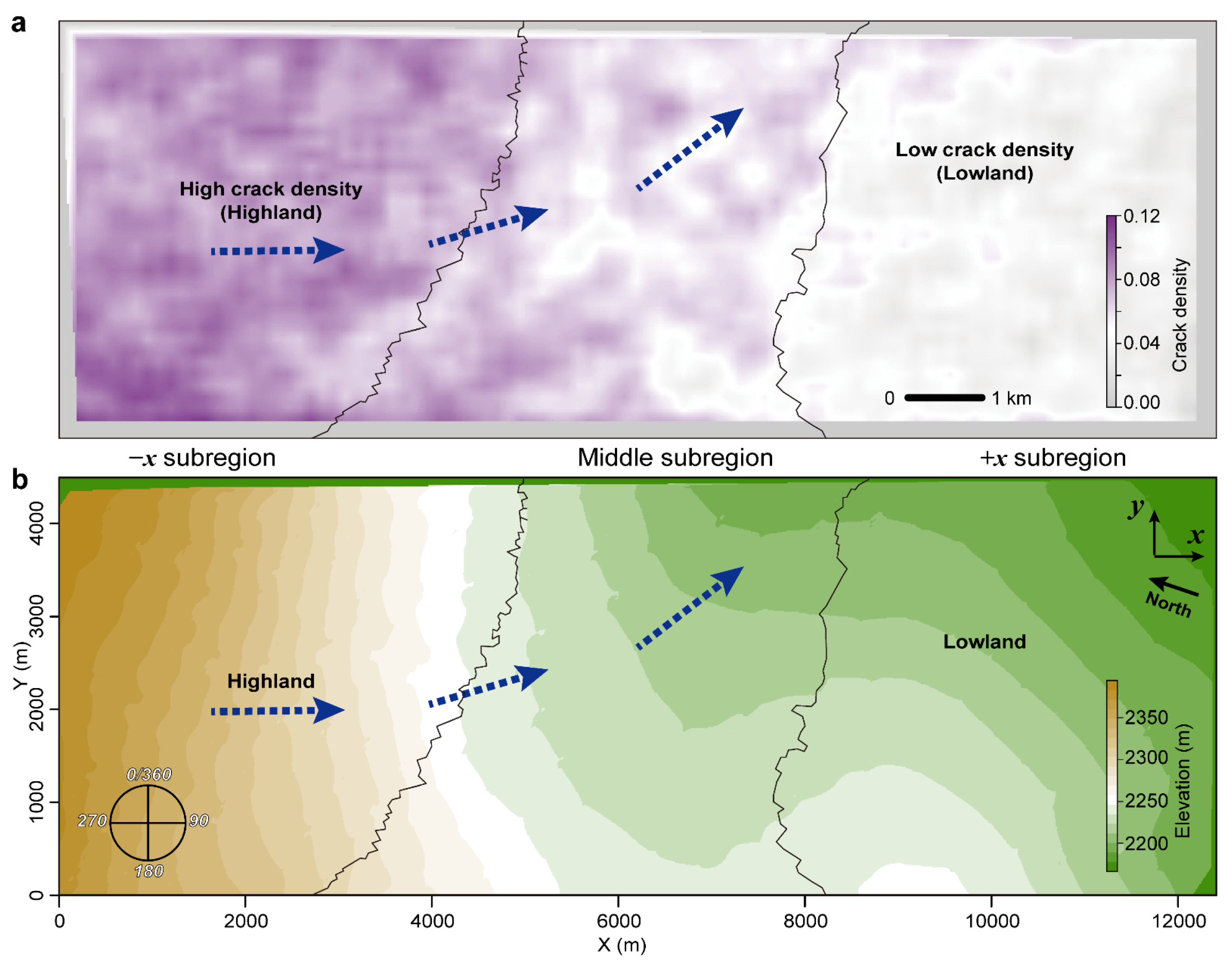
3.3. Polygon Edge Density Distribution of the Polygons

Based on the method proposed in Section 2.2, we can individually calculate the polygon edge density in each local region. Figure 5a presents the distribution of the calculated polygon edge density, showing three subregions consistent with that in Figure 3a and Figure 4a. The average polygon edge densities of the –x, middle and +x subregions are ~0.10, ~0.06, and ~0.03, respectively.

Figure 5b shows the elevation distribution around the analyzed polygonal terrain in the Cartesian coordinate system. Obviously, within the region of x = 0–3000 m, the elevation is over 2300 m, representing a “highland” in the –x subregion. In the region of x = 8000–12,000 m, a slope is descending to the ~45-degree direction. The distribution of polygon edge density has been experimentally proved to be related to the salt content [22,23]. The –x subregion has a relatively higher polygon edge density (lower salt content) than the +x subregion.

4. Discussions

4.1. Possible Formation Mechanisms of the Three-Subregion Zone

As observed in Section 3, the three subregions show different geometric properties in polygonal size, area, and orientation. A possible mechanism for the formation of this special tripartite region is that the ice cap on the slope (–x subregion, Figure 5b) is unstable and deforms slowly towards the lowland through long-term surface creep, but the sliding direction would be caused by gravity, and the surrounding terrains would block the polygons. As a result, the polygons align in nearly parallel directions along their moving direction, forming an ice transportation band system (middle subregion, Figure 3a and Figure 5b).

4.2. Different Polygon Edge Density Distribution

Polygon edge density might reflect the salt activity in the medium [22,23]. Higher salt contents might respond to lower polygon edge densities according to the experimental results based on NaCl [23,25]. The Martian surface is thought to contain salt or saline materials [30,31,32]. The correlation of the size-dependent polygonal surface structure occurrences and elevations indicates that the formation of polygons is influenced by mineralogy [33]. According to the calculated polygon edge density distribution (Figure 5a), the polygon edge density in the highland is systematically larger than that in the lowland, with a transition zone in the middle, which can be explained by the concentration of salt minerals in lowlands so that the growth of fracturing is inhibited [34].

Furthermore, other possible mechanisms could explain the different polygon sizes and/or polygon edge density distribution. For example, different thicknesses of the cracking layer could influence polygon patterns [35], or even the rate/speed of deformation might modify polygon size. However, due to the lack of information from in situ observations, the crack properties (e.g., material composition) in this region cannot be well constrained. With more observation of the satellite spectrum, the investigation of the material composition on the southern polar cap of Mars would be improved, thus providing more constraints for studying the ancient and present climate of Mars.

4.3. Implication of Water/ice Activity on Polar Regions

Martian polar caps are crucial to the investigation of water/ice activity on Mars. The evidence of liquid water in Mars’ subsurface has been discovered near the southern ice cap [36]. The possibly existing flowing water under the ice may also participate in the healing of the ice at the top. However, considering the extremely low temperature on the surface [37] and in the subsurface [38,39] at the South Pole of Mars, liquid water (with zero or low salt content) is hard to exist on the near-surface; thus, the explanation of flowing water under the ice can be ruled out. In addition, polar caps also present ablation features around the rims, showing a receding of the ice caps during the hotter seasons [40]. In addition to analyzing the HiRISE image of polygonal terrains, studies of Martian meteorites or in-situ observations can provide more constraints on the water/ice-related terrain on Mars. Specifically, the interaction of water in ancient terrains on Mars can additionally obtain constraints from the study of meteorites [41]. The processes of formation of carbonates in the cracks of rocks such as ALH84001 are described [42].

5. Conclusions

Based on the recognition of the polygons in a polygonal terrain on the southern polar cap of Mars, three subregions can be distinguished according to the distributions of polygon size, elongation orientation and polygon edge density. In addition, the –x and the +x subregions distribute relatively small and relatively large polygons, respectively, and the middle subregion can be regarded as an intermediate zone along the slope. This intermediate zone is squeezed by the surrounding polygons, indicating that surface creep and/or uplift or subsidence (e.g., glacier movement) [43,44] might be possible on earlier and present Mars. Topography controls the elongation orientation of these polygons, which indicates that polar ice-cap polygons are formed in the process of lateral sliding, and there are complex processes, such as healing, at the long-term contact boundaries.

References

1. Hiesinger, H.; Head III, J.W. Characteristics and origin of polygonal terrain in southern Utopia Planitia, Mars: Results from Mars Orbiter Laser Altimeter and Mars Orbiter Camera data. J. Geophys. Res. Planets 2000, 105, 11999–12022. [Google Scholar] [CrossRef]
2. Brooker, L.M.; Balme, M.R.; Conway, S.J.; Hagermann, A.; Barrett, A.M.; Collins, G.S.; Soare, R.J. Clastic polygonal networks around Lyot crater, Mars: Possible formation mechanisms from morphometric analysis. Icarus 2018, 302, 386–406. [Google Scholar] [CrossRef]
3. Morison, A.; Labrosse, S.; Choblet, G. Sublimation-driven convection in Sputnik Planitia on Pluto. Nature 2021, 600, 419–423. [Google Scholar] [CrossRef] [PubMed]
4. Yoshikawa, K. Origin of the polygons and the thickness of Vastitas Borealis Formation in Western Utopia Planitia on Mars. Geophys. Res. Lett. 2003, 30, 5-1–5-4. [Google Scholar] [CrossRef]
5. Mangold, N. High latitude patterned grounds on Mars: Classification, distribution and climatic control. Icarus 2005, 174, 336–359. [Google Scholar] [CrossRef]
6. Morgenstern, A.; Hauber, E.; Reiss, D.; van Gasselt, S.; Grosse, G.; Schirrmeister, L. Deposition and degradation of a volatile-rich layer in Utopia Planitia and implications for climate history on Mars. J. Geophys. Res. Planets 2007, 112, E06010. [Google Scholar] [CrossRef] [Green Version]
7. Levy, J.; Head, J.; Marchant, D. Thermal contraction crack polygons on Mars: Classification, distribution, and climate implications from HiRISE observations. J. Geophys. Res. Planets 2009, 114, E01007. [Google Scholar] [CrossRef] [Green Version]
8. Orgel, C.; Hauber, E.; van Gasselt, S.; Reiss, D.; Johnsson, A.; Ramsdale, J.D.; Smith, I.; Swirad, Z.M.; Séjourné, A.; Wilson, J.T.; et al. Grid mapping the northern plains of Mars: A new overview of recent water-and ice-related landforms in Acidalia Planitia. J. Geophys. Res. Planets 2019, 124, 454–482. [Google Scholar] [CrossRef] [Green Version]
9. Séjourné, A.; Costard, F.; Swirad, Z.M.; Łosiak, A.; Bouley, S.; Smith, I.; Balme, M.R.; Orgel, C.; Ramsdale, J.D.; Hauber, E.; et al. Grid mapping the Northern Plains of Mars: Using morphotype and distribution of ice-related landforms to understand multiple ice-rich deposits in Utopia Planitia. J. Geophys. Res. Planets 2019, 124, 483–503. [Google Scholar] [CrossRef] [Green Version]
10. Mellon, M.T. Small-scale polygonal features on Mars: Seasonal thermal contraction cracks in permafrost. J. Geophys. Res. Planets 1997, 102, 25617–25628. [Google Scholar] [CrossRef]
11. Seibert, N.M.; Kargel, J.S. Small-scale Martian polygonal terrain: Implications for liquid surface water. Geophys. Res. Lett. 2001, 28, 899–902. [Google Scholar] [CrossRef]
12. Lu, Y.; Liu, S.; Weng, L.; Wang, L.; Li, Z.; Xu, L. Fractal analysis of cracking in a clayey soil under freeze–thaw cycles. Eng. Geol. 2016, 208, 93–99. [Google Scholar] [CrossRef]
13. Kieffer, H.H. Mars south polar spring and summer temperatures: A residual CO2 frost. J. Geophys. Res. Solid Earth 1979, 84, 8263–8288. [Google Scholar] [CrossRef]
14. Byrne, S.; Ingersoll, A.P. A sublimation model for Martian south polar ice features. Science 2003, 299, 1051–1053. [Google Scholar] [CrossRef] [PubMed] [Green Version]
15. Phillips, R.J.; Davis, B.J.; Tanaka, K.L.; Byrne, S.; Mellon, M.T.; Putzig, N.E.; Haberle, R.M.; Kahre, M.A.; Campbell, B.A.; Carter, L.M.; et al. Massive CO2 ice deposits sequestered in the south polar layered deposits of Mars. Science 2011, 332, 838–841. [Google Scholar] [CrossRef] [PubMed] [Green Version]
16. Jian, J.-J.; Ip, W.-H. Seasonal patterns of condensation and sublimation cycles in the cryptic and non-cryptic regions of the South Pole. Adv. Space Res. 2009, 43, 138–142. [Google Scholar] [CrossRef]
17. Portyankina, G.; Pommerol, A.; Aye, K.M.; Hansen, C.J.; Thomas, N. Polygonal cracks in the seasonal semi-translucent CO2 ice layer in Martian polar areas. J. Geophys. Res. Planets 2012, 117, E02006. [Google Scholar] [CrossRef] [Green Version]
18. McGill, G.E.; Hills, L.S. Origin of giant Martian polygons. J. Geophys. Res. Planets 1992, 97, 2633–2647. [Google Scholar] [CrossRef]
19. Lefort, A.; Russell, P.S.; Thomas, N.; McEwen, A.S.; Dundas, C.M.; Kirk, R.L. Observations of periglacial landforms in Utopia Planitia with the high resolution imaging science experiment (HiRISE). J. Geophys. Res. Planets 2009, 114, E04005. [Google Scholar] [CrossRef] [Green Version]
20. Buczkowski, D.L.; Seelos, K.D.; Cooke, M.L. Giant polygons and circular graben in western Utopia basin, Mars: Exploring possible formation mechanisms. J. Geophys. Res. Planets 2012, 117, E08010. [Google Scholar] [CrossRef]
21. Ulrich, M.; Hauber, E.; Herzschuh, U.; Härtel, S.; Schirrmeister, L. Polygon pattern geomorphometry on Svalbard (Norway) and western Utopia Planitia (Mars) using high-resolution stereo remote-sensing data. Geomorphology 2011, 134, 197–216. [Google Scholar] [CrossRef] [Green Version]
22. DeCarlo, K.F.; Shokri, N. Salinity effects on cracking morphology and dynamics in 3-D desiccating clays. Water Resour. Res. 2014, 50, 3052–3072. [Google Scholar] [CrossRef]
23. Shokri, N.; Zhou, P.; Keshmiri, A. Patterns of desiccation cracks in saline bentonite layers. Transp. Porous Media 2015, 110, 333–344. [Google Scholar] [CrossRef]
24. Yang, B.; Yuan, J. Influence of soda content on desiccation cracks in clayey soils. Soil Sci. Soc. Am. J. 2019, 83, 1054–1061. [Google Scholar] [CrossRef]
25. Li, D.; Yang, B.; Yang, C.; Zhang, Z.; Hu, M. Effects of salt content on desiccation cracks in the clay. Environ. Earth Sci. 2021, 80, 671. [Google Scholar] [CrossRef]
26. Van Gasselt, S.; Reiss, D.; Thorpe, A.K.; Neukum, G. Seasonal variations of polygonal thermal contraction crack patterns in a south polar trough, Mars. J. Geophys. Res. Planets 2005, 110, E08002. [Google Scholar] [CrossRef] [Green Version]
27. Kossacki, K.J.; Markiewicz, W.J.; Smith, M.D. Surface temperature of Martian regolith with polygonal features: Influence of the subsurface water ice. Planet. Space Sci. 2003, 51, 569–580. [Google Scholar] [CrossRef]
28. Van Gasselt, S.; Hao, J. Systematic High-Resolution Remote-Sensing Investigation of Martian South Polar Landforms: Thermal Contraction Polygons. In EGU General Assembly Conference Abstracts; EGU General Assembly: Vienna, Austria, 2015; p. 7819. [Google Scholar]
29. McEwen, A.S.; Eliason, E.M.; Bergstrom, J.W.; Bridges, N.T.; Hansen, C.J.; Delamere, W.A.; Grant, J.A.; Gulick, V.C.; Herkenhoff, K.E.; Keszthelyi, L.; et al. Mars reconnaissance orbiter’s high resolution imaging science experiment (HiRISE). J. Geophys. Res. Planets 2007, 112, E05S02. [Google Scholar] [CrossRef] [Green Version]
30. Möhlmann, D.; Thomsen, K. Properties of cryobrines on Mars. Icarus 2011, 212, 123–130. [Google Scholar] [CrossRef]
31. Martín-Torres, F.J.; Zorzano, M.-P.; Valentín-Serrano, P.; Harri, A.-M.; Genzer, M.; Kemppinen, O.; Rivera-Valentin, E.G.; Jun, I.; Wray, J.; Madsen, M.B.; et al. Transient liquid water and water activity at Gale crater on Mars. Nat. Geosci. 2015, 8, 357–361. [Google Scholar] [CrossRef]
32. Rivera-Valentín, E.G.; Chevrier, V.F.; Soto, A.; Martínez, G. Distribution and habitability of (meta) stable brines on present-day Mars. Nat. Astron. 2020, 4, 756–761. [Google Scholar] [CrossRef] [PubMed]
33. Dang, Y.N.; Xiao, L.; Xu, Y.; Zhang, F.; Huang, J.; Wang, J.; Zhao, J.N.; Komatsu, G.; Yue, Z. The polygonal surface structures in the Dalangtan Playa, Qaidam Basin, NW China: Controlling factors for their formation and implications for analogous Martian landforms. J. Geophys. Res. Planets 2018, 123, 1910–1933. [Google Scholar] [CrossRef]
34. Dang, Y.; Zhang, F.; Zhao, J.; Wang, J.; Xu, Y.; Huang, T.; Xiao, L. Diverse polygonal patterned grounds in the northern Eridania basin, Mars: Possible origins and implications. J. Geophys. Res. Planets 2020, 125, e2020JE006647. [Google Scholar] [CrossRef]
35. Nandakishore, P.; Goehring, L. Crack patterns over uneven substrates. Soft Matter 2016, 12, 2253–2263. [Google Scholar] [CrossRef] [Green Version]
36. Orosei, R.; Lauro, S.E.; Pettinelli, E.; Cicchetti, A.; Coradini, M.; Cosciotti, B.; Di Paolo, F.; Flamini, E.; Mattei, E.; Pajola, M.; et al. Radar evidence of subglacial liquid water on Mars. Science 2018, 361, 490–493. [Google Scholar] [CrossRef] [Green Version]
37. Forget, F.; Hourdin, F.; Fournier, R.; Hourdin, C.; Talagrand, O.; Collins, M.; Lewis, S.R.; Read, P.L.; Huot, J.P. Improved general circulation models of the Martian atmosphere from the surface to above 80 km. J. Geophys. Res. Planets 1999, 104, 24155–24175. [Google Scholar] [CrossRef]
38. Price, P.B.; Nagornov, O.V.; Bay, R.; Chirkin, D.; He, Y.; Miocinovic, P.; Richards, A.; Woschnagg, K.; Koci, B.; Zagorodnov, V. Temperature profile for glacial ice at the South Pole: Implications for life in a nearby subglacial lake. Proc. Natl. Acad. Sci. USA 2002, 99, 7844–7847. [Google Scholar] [CrossRef] [Green Version]
39. Zhang, L.; Zhang, J.; Mitchell, R.N.; Cao, P.; Liu, J. A thermal origin for super-high-frequency marsquakes. Icarus 2023, 390, 115327. [Google Scholar] [CrossRef]
40. Smith, D.E.; Zuber, M.T.; Frey, H.V.; Garvin, J.B.; Head, J.W.; Muhleman, D.O.; Pettengill, G.H.; Phillips, R.J.; Solomon, S.C.; Zwally, H.J.; et al. Topography of the northern hemisphere of Mars from the Mars Orbiter Laser Altimeter. Science 1998, 279, 1686–1692. [Google Scholar] [CrossRef] [Green Version]
41. Bridges, J.C.; Catling, D.C.; Saxton, J.M.; Swindle, T.D.; Lyon, I.C.; Grady, M.M. Alteration assemblages in Martian meteorites: Implications for near-surface processes. Space Sci. Rev. 2001, 96, 365–392. [Google Scholar] [CrossRef]
42. Moyano-Cambero, C.E.; Trigo-Rodríguez, J.M.; Benito, M.I.; Alonso-Azcárate, J.; Lee, M.R.; Mestres, N.; Martínez-Jiménez, M.; Martín-Torres, F.J.; Fraxedas, J. Petrographic and geochemical evidence for multiphase formation of carbonates in the Martian orthopyroxenite Allan Hills 84001. Meteorit. Planet. Sci. 2017, 52, 1030–1047. [Google Scholar] [CrossRef] [Green Version]
43. Sleep, N.H. Martian plate tectonics. J. Geophys. Res. Planets 1994, 99, 5639–5655. [Google Scholar] [CrossRef]
44. Clark, B.R.; Mullin, R.P. Martian glaciation and the flow of solid CO2. Icarus 1976, 27, 215–228. [Google Scholar] [CrossRef]
Figure 1. The study region with Martian polygonal terrain on the southern polar cap. (a) Martian topographic map centered on the south pole. The topography is exaggerated for better visualization. (b) Enlargement view for a region of the ice cap. The white rectangle indicates the region shown in (c). (c) The image of the polygonal terrain, taken by HiRISE (ID: ESP_039633_0950). Image credit of HiRISE: NASA/JPL/University of Arizona. The elevation data was obtained from The Mars Orbiter Laser Altimeter (MOLA) database (https://attic.gsfc.nasa.gov/mola/ (accessed on 1 September 2022)).
Remotesensing 14 05789 g001
Figure 3. The analysis of polygon areas. (a) Distribution of the polygon areas. The entire region is divided into three subregions (–x, middle, and +x subregions), approximately separated by the boundaries of the individual polygons (the white lines). (bd) Three representative enlarged HiRISE images of the polygonal terrains in the subregions, where their locations are marked in (a). (eg) Histograms showing the number of different area polygon areas in the three subregions. The mean values of the areas are marked.
Remotesensing 14 05789 g003
Figure 4. The analysis distribution of elongation orientation of the polygons. (a) Distribution of elongation orientation of the polygons in three subregions. (bd) Windrose plots of elongation orientations in the three subregions. Dominate elongation orientations are marked with arrows.
Remotesensing 14 05789 g004
Figure 5. The illustration of possible uplift or subsidence. (a) Distribution of polygon edge density. (b) Elevation distribution, obtained from the MOLA database (https://attic.gsfc.nasa.gov/mola/ (accessed on 1 September 2022)). A set of dashed arrows from the highland to the lowland indicate the possible direction of the uplift or subsidence.
Remotesensing 14 05789 g005
Publisher’s Note: MDPI stays neutral with regard to jurisdictional claims in published maps and institutional affiliations.