Semantic Segmentation and 3D Reconstruction of Concrete Cracks


Abstract
:
1. Introduction
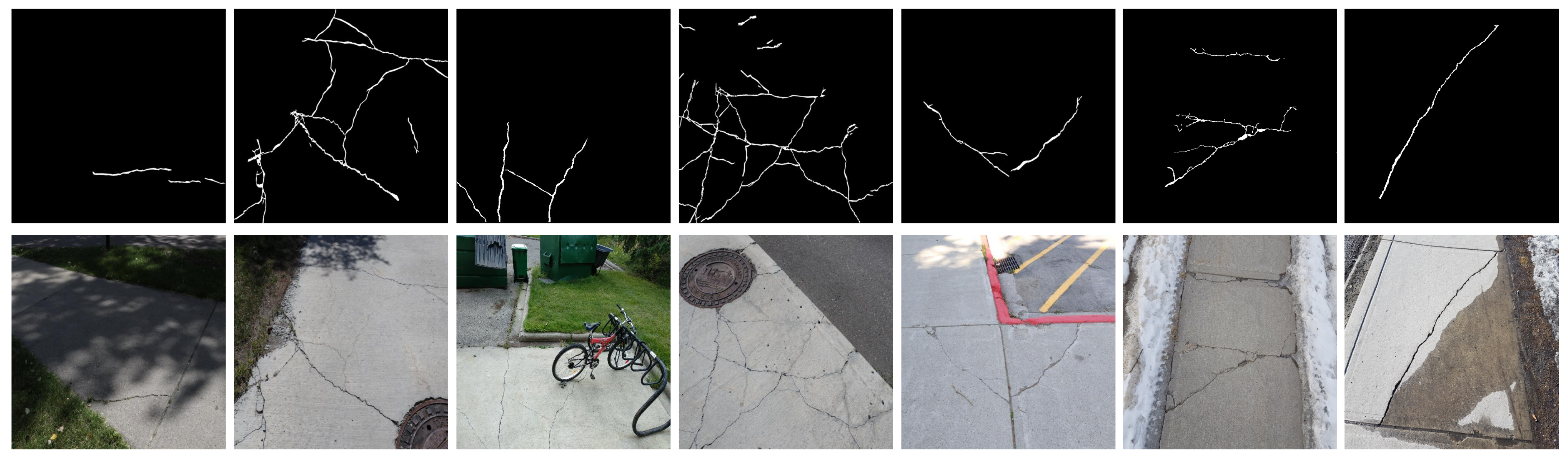
- Addressing data inadequacy challenges by producing a challenging and complex dataset for crack segmentation, including images with various resolutions and with a variety of crack shapes/sizes, then developing a semi-supervised data annotation approach and investigating the potential of GAN-based data augmentation.
- Investigating crack segmentation issues by benchmarking the performance of four state-of-the-art semantic segmentation approaches (SegNet, UNet, Attention Res-UNet, and SP) for identifying cracks; validating the impact of various data augmentation approaches; testing the sensitivity of the models to image scale and resolution; and proposing the use of a loss function based on Intersection of Union (IoU) to reduce the impact of class imbalance on model performance.
- Proposing a new calibration model for calibrating a commercial stereo camera (ZED by Stereolabs); and investigating single-image and stereo 3D reconstruction of segmented cracks based on planarity assumptions and stereo inference, respectively.
2. Methodology
2.1. Dataset Preparation and Augmentation
2.2. Semantic Segmentation Architectures
2.2.1. SegNet
2.2.2. UNet
2.2.3. Structured Prediction
2.3. Training Details
2.3.1. Transfer Learning
2.3.2. Early Stopping
2.3.3. Loss Functions
2.4. Statistical Significance
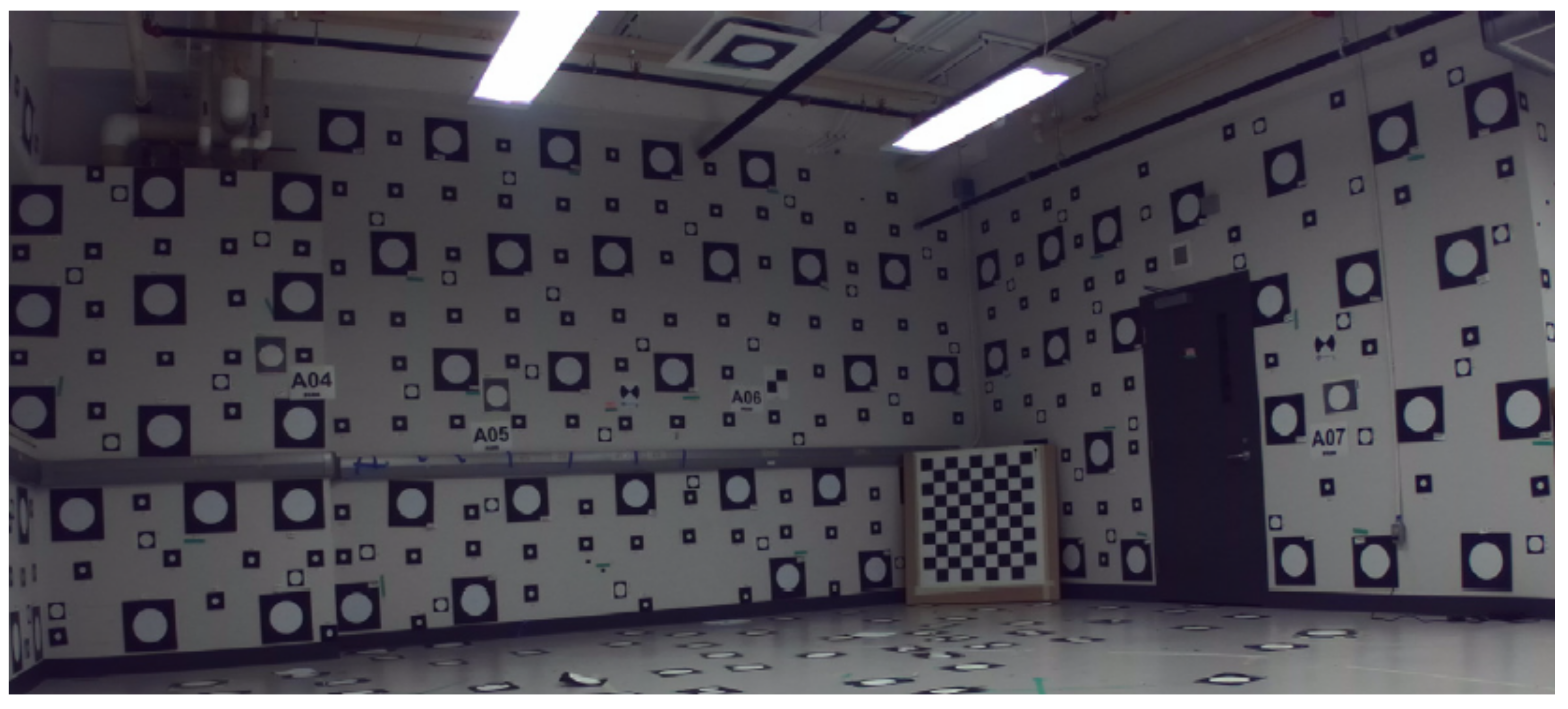
2.5. Calibration
Calibration Model
2.6. 3D Reconstruction
2.6.1. Planar Approach
2.6.2. Stereo Inference Approach
3. Experiments and Results
3.1. Synthetic Image/Label Generation by GANs
3.2. Semantic Segmentation
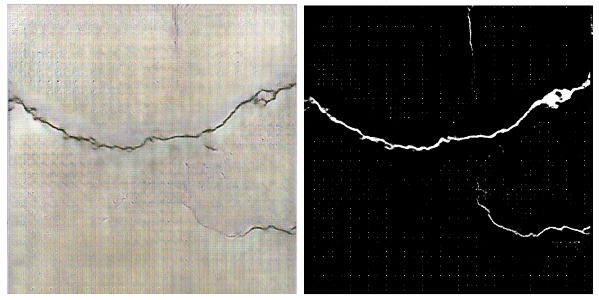
Qualitative Assessment
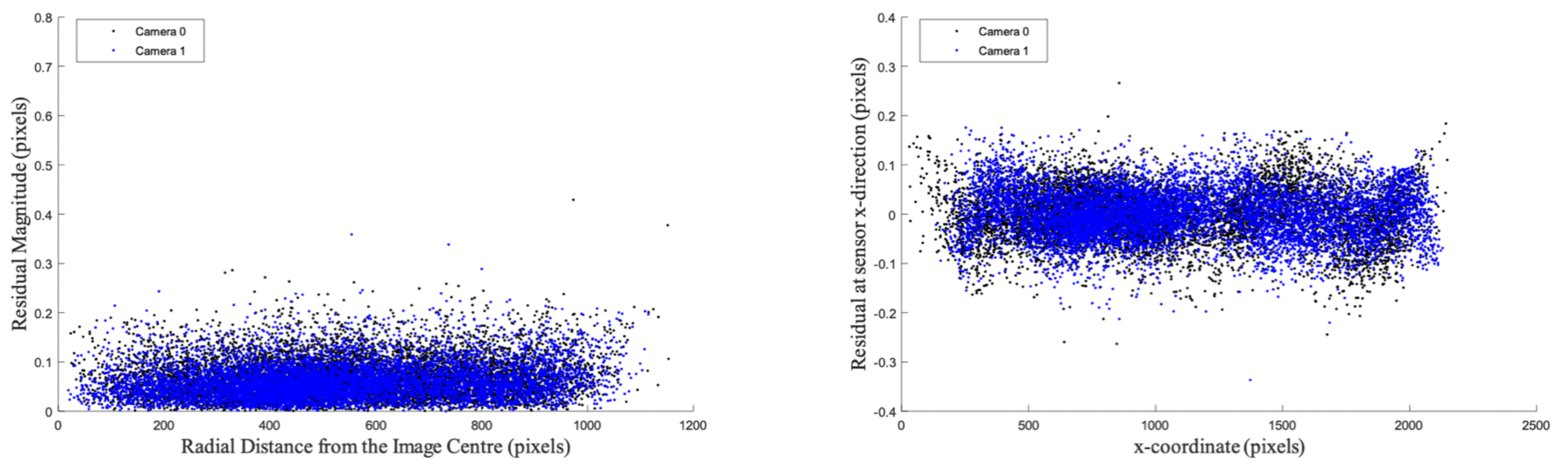
3.3. Calibration
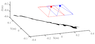
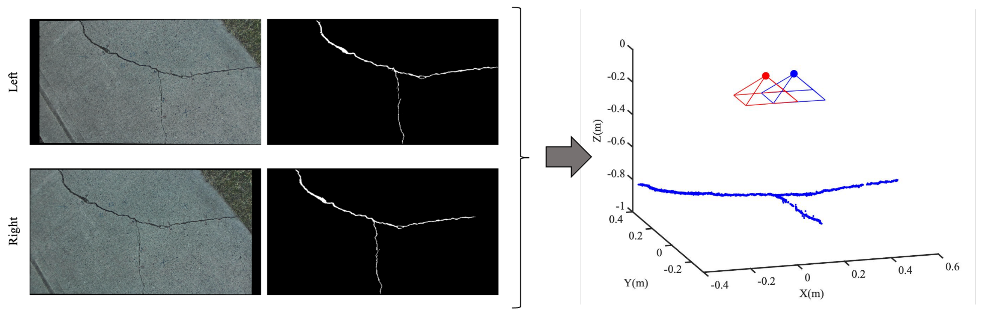
3.4. 3D Reconstruction
3.4.1. Qualitative Evaluation
3.4.2. Quantitative Assessment
4. Discussion
- How can the problem of data inadequacy in training semantic segmentation networks to identify cracks be overcome?In addition to collecting a rich dataset containing various types of images, data augmentation techniques were used in this research. During our experiments, it was shown that although GAN augmentation can be helpful in certain cases, the traditional augmentation techniques are more reliable, guaranteeing either boosted performance, or at the very least, not reducing the performance of the semantic segmentation networks. The other approach that helped with data inadequacy was using information from a different segmentation task to pre-train the segmentation network on a large dataset such as ImageNet. In future studies, domain adaptation should be considered.
- How can the class imbalance issue for crack segmentation be dealt with?The CCSS-DATA dataset is naturally imbalanced, as the number of crack pixels in each image is higher than the background pixels, and adding images with no cracks intensifies the overall imbalance. Therefore, choosing the Jaccard loss function instead of the BCE loss ensured higher performance with the same data.
- What considerations should be made in order to develop a semantic segmentation approach that can detect cracks at different scales?In seeking to develop a scale-invariant model, adding smaller zoomed-in image patches to the training dataset before resizing the training samples was helpful. This helped the network detect multiple scales of objects with the same amount of collected data.
- Do the semantic segmentation networks work well in outdoor environments with varied lighting conditions, ambiguous texture patterns, and high resolution images covering a large field of view?The inference images of the collected dataset (CCSS-DATA) include many challenging scenes, such as shadows and background objects, and cover a large field of view. As shown in this study, the UNet and SegNet networks had decent performance on these test scenes.
- Are the calibration parameters provided by the stereo camera’s manufacturer sufficient for reconstructing the cracks? If not, what is the best calibration model for the stereo camera?No, the calibration parameters provided by Stereo Labs were not sufficient to accurately model the cracks. Therefore, modifications were applied to the calibration model to ensure that the distortion parameters and RO parameters of the stereo camera were accurately estimated.
- What is the best crack reconstruction approach considering the semantic segmentation results and a well-calibrated stereo camera?Assuming prior knowledge that the surface of the concrete is planar, the planar 3D modeling approach was the fastest algorithm. Otherwise, the matching approach was more accurate, and does not require the concrete surface surrounding the crack to be planar.
5. Conclusions
Author Contributions
Funding
Data Availability Statement
Conflicts of Interest
Abbreviations
| CNN | Convolutional Neural Network |
| GAN | Generative Adversarial Network |
| CCSS-DATA | Concrete Cracks Semantic Segmentation Dataset |
| DCGAN | Deep Convolutional Generative Adversarial Network |
| ProGAN | Progressive Growing of Generative Adversarial Network |
| EOP | Exterior Orientation Parameter |
| IOP | Interior Orientation Parameter |
| UNet | A type of semantic segmentation neural network |
| SegNet | A type of semantic segmentation neural network |
| ResNet | Residual Network |
| IoU | Intersection over Union |
| F1 | F1 Score, an evaluation metric |
| P | Precision |
| R | Recall |
| BCE | Binary Cross-Entropy |
| 3D | three-dimensional |
| StD | Standard Deviation |
| RMS | Root-Mean-Square |
| RGB | Red-Green-Blue |
| DSLR | Digital Single-Lens Reflex |
| SfM | Structure from Motion |
Appendix A
Appendix A.1

Appendix A.2

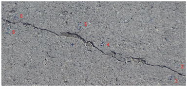
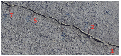
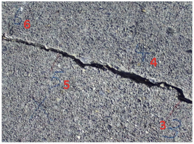
| Left Image in Stereo Pair | Marks | Ground Truth Distance (mm) | Matching Error (mm) | Planar Error (mm) |
|---|---|---|---|---|
 | 5–6 7–8 | 8.25 9.45 | −1.26 −0.68 | −4.79 −2.31 |
 | 1–2 3–5 6–9 | 2.8 92.6 99.6 | 0.64 −0.9 0.61 | 0.56 −0.24 0.5 |
 | 2–3 4–5 6–8 9–10 11–12 | 20.2 80.5 94.3 24.1 94 | 0.51 1.2 1.32 1.18 −0.53 | 0.53 1.4 1.31 0.55 −0.77 |
 | 1–2 5–6 7–8 | 12.4 117 17.7 | 1.24 0.05 0.88 | 1.15 0.33 0.82 |
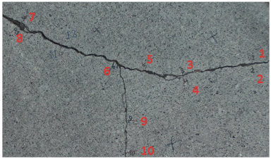 | 1–2 3–4 5–6 7–8 9–10 | 5 7.3 87.2 17.2 92 | 0.72 1.33 0.72 −0.57 1.11 | 1.1 0.56 0.31 −0.35 0.04 |
 | 1–2 3–4 5–6 | 137.3 9.1 149.4 | −0.53 0.92 −0.08 | −0.6 0.88 −0.71 |
 | 1–2 5–7 | 114.9 123.9 | 0.35 0.53 | 0.32 0.59 |
 | 1–2 4–5 8–10 9–10 | 10.8 143.3 137.8 12.2 | 0.77 0.73 0.63 0.29 | 0.8 0.86 0.9 0.2 |
 | 3–4 5–6 | 109.45 110.6 | 1.17 0.85 | −0.38 1.29 |
 | 1–2 5–6 3–4 | 141.1 95.5 143 | 0.07 1.07 1.39 | 0.37 0.54 2.1 |
| RMS | 0.86 | 1.23 | ||
| StD(abs) | 0.3798 | 0.8755 |
Appendix A.3
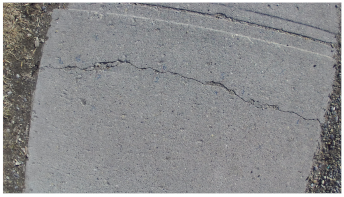
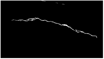
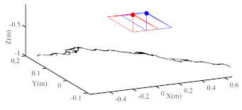
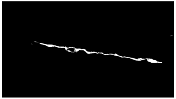
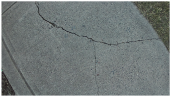
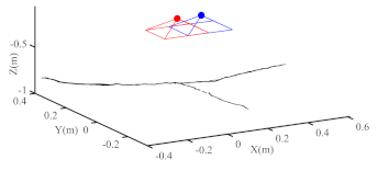
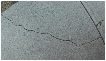
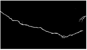
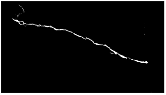
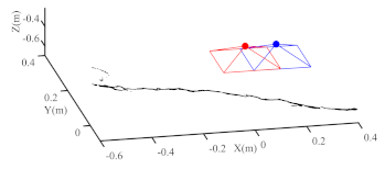
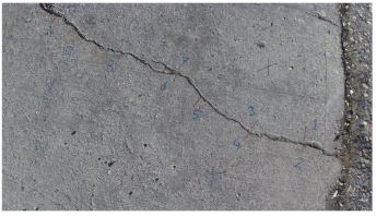
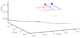
| Left Image in Stereo Pair | Left Segmented Crack | 3D Reconstructed Crack |
|---|---|---|
 |  |  |
 |  |  |
 |  |  |
 |  |  |
 |  |  |
 |  |  |
 |  |  |
 |  |  |
 |  |  |
 |  |  |
References
- Saatcioglu, M.; Ghobarah, A.; Nistor, I. Effects of the December 26, 2004 Sumatra earthquake and tsunami on physical infrastructure. ISET J. Earthq. Technol. 2005, 42, 79–94. [Google Scholar]
- Hassanain, M.A.; Loov, R.E. Cost optimization of concrete bridge infrastructure. Can. J. Civ. Eng. 2003, 30, 841–849. [Google Scholar] [CrossRef]
- Yu, S.N.; Jang, J.H.; Han, C.S. Auto inspection system using a mobile robot for detecting concrete cracks in a tunnel. Autom. Constr. 2007, 16, 255–261. [Google Scholar] [CrossRef]
- Oh, J.K.; Jang, G.; Oh, S.; Lee, J.H.; Yi, B.J.; Moon, Y.S.; Lee, J.S.; Choi, Y. Bridge inspection robot system with machine vision. Autom. Constr. 2009, 18, 929–941. [Google Scholar] [CrossRef]
- Montero, R.; Victores, J.; Martinez, S.; Jardón, A.; Balaguer, C. Past, present and future of robotic tunnel inspection. Autom. Constr. 2015, 59, 99–112. [Google Scholar] [CrossRef]
- Lee, D.; Kim, J.; Lee, D. Robust Concrete Crack Detection Using Deep Learning-Based Semantic Segmentation. Int. J. Aeronaut. Space Sci. 2019, 20, 287–299. [Google Scholar] [CrossRef]
- Jahanshahi, M.R.; Masri, S.F.; Padgett, C.W.; Sukhatme, G.S. An innovative methodology for detection and quantification of cracks through incorporation of depth perception. Mach. Vis. Appl. 2013, 24, 227–241. [Google Scholar] [CrossRef]
- Kim, B.; Cho, S. Automated vision-based detection of cracks on concrete surfaces using a deep learning technique. Sensors 2018, 18, 3452. [Google Scholar] [CrossRef] [Green Version]
- Fan, Z.; Wu, Y.; Lu, J.; Li, W. Automatic pavement crack detection based on structured prediction with the convolutional neural network. arXiv 2018, arXiv:1802.02208. [Google Scholar]
- Hedayati, M.; Sofi, M.; Mendis, P.; Ngo, T. A Comprehensive Review of Spalling and Fire Performance of Concrete Members. Electron. J. Struct. Eng. 2015, 15, 8–34. [Google Scholar] [CrossRef]
- Greening, N.; Landgren, R. Surface Discoloration of Concrete Flatwork; Number 203; Portland Cement Association, Research and Development Laboratories: Skokie, IL, USA, 1966. [Google Scholar]
- Jahanshahi, M.R.; Masri, S.F. A new methodology for non-contact accurate crack width measurement through photogrammetry for automated structural safety evaluation. Smart Mater. Struct. 2013, 22, 035019. [Google Scholar] [CrossRef]
- Chambon, S.; Moliard, J.M. Automatic road pavement assessment with image processing: Review and comparison. Int. J. Geophys. 2011, 2011, 989354. [Google Scholar] [CrossRef]
- Shan, B.; Zheng, S.; Ou, J. A stereovision-based crack width detection approach for concrete surface assessment. KSCE J. Civ. Eng. 2016, 20, 803–812. [Google Scholar] [CrossRef]
- Shi, Y.; Cui, L.; Qi, Z.; Meng, F.; Chen, Z. Automatic road crack detection using random structured forests. IEEE Trans. Intell. Transp. Syst. 2016, 17, 3434–3445. [Google Scholar] [CrossRef]
- Fan, Y.; Zhao, Q.; Ni, S.; Rui, T.; Ma, S.; Pang, N. Crack detection based on the mesoscale geometric features for visual concrete bridge inspection. J. Electron. Imaging 2018, 27, 053011. [Google Scholar] [CrossRef]
- Hoskere, V.; Narazaki, Y.; Hoang, T.; Spencer, B., Jr. Vision-based structural inspection using multiscale deep convolutional neural networks. arXiv 2018, arXiv:1805.01055. [Google Scholar]
- Liskowski, P.; Krawiec, K. Segmenting retinal blood vessels with deep neural networks. IEEE Trans. Med. Imaging 2016, 35, 2369–2380. [Google Scholar] [CrossRef]
- Cha, Y.J.; Choi, W.; Büyüköztürk, O. Deep learning-based crack damage detection using convolutional neural networks. Comput.-Aided Civ. Infrastruct. Eng. 2017, 32, 361–378. [Google Scholar] [CrossRef]
- Cao, M.T.; Tran, Q.V.; Nguyen, N.M.; Chang, K.T. Survey on performance of deep learning models for detecting road damages using multiple dashcam image resources. Adv. Eng. Inform. 2020, 46, 101182. [Google Scholar] [CrossRef]
- Ronneberger, O.; Fischer, P.; Brox, T. U-net: Convolutional networks for biomedical image segmentation. In Proceedings of the International Conference on Medical Image Computing and Computer-Assisted Intervention, Munich, Germany, 5–9 October 2015; pp. 234–241. [Google Scholar]
- Badrinarayanan, V.; Kendall, A.; Cipolla, R. Segnet: A deep convolutional encoder-decoder architecture for image segmentation. IEEE Trans. Pattern Anal. Mach. Intell. 2017, 39, 2481–2495. [Google Scholar] [CrossRef]
- Lau, S.L.; Chong, E.K.; Yang, X.; Wang, X. Automated pavement crack segmentation using u-net-based convolutional neural network. IEEE Access 2020, 8, 114892–114899. [Google Scholar] [CrossRef]
- Lin, F.; Yang, J.; Shu, J.; Scherer, R.J. Crack Semantic Segmentation using the U-Net with Full Attention Strategy. arXiv 2021, arXiv:2104.14586. [Google Scholar]
- Vaswani, A.; Shazeer, N.; Parmar, N.; Uszkoreit, J.; Jones, L.; Gomez, A.N.; Kaiser, Ł.; Polosukhin, I. Attention is all you need. arXiv 2017, arXiv:1706.03762. [Google Scholar]
- Hsiel, Y.A.; Tsai, Y.C.J. Dau-net: Dense attention u-net for pavement crack segmentation. In Proceedings of the 2021 IEEE International Intelligent Transportation Systems Conference (ITSC), Indianapolis, IN, USA, 19–22 September 2021; pp. 2251–2256. [Google Scholar]
- Song, C.; Wu, L.; Chen, Z.; Zhou, H.; Lin, P.; Cheng, S.; Wu, Z. Pixel-level crack detection in images using SegNet. In Multi-Disciplinary Trends in Artificial Intelligence. MIWAI 2019; Lecture Notes in Computer Science; Springer: Cham, Switzerland, 2019; pp. 247–254. [Google Scholar]
- Canny, J. A Computational Approach to Edge Detection. IEEE Trans. Pattern Anal. Mach. Intell. 1986, PAMI-8, 679–698. [Google Scholar] [CrossRef]
- Kanopoulos, N.; Vasanthavada, N.; Baker, R. Design of an image edge detection filter using the Sobel operator. IEEE J. Solid-State Circuits 1988, 23, 358–367. [Google Scholar] [CrossRef]
- Chen, T.; Cai, Z.; Zhao, X.; Chen, C.; Liang, X.; Zou, T.; Wang, P. Pavement crack detection and recognition using the architecture of segNet. J. Ind. Inf. Integr. 2020, 18, 100144. [Google Scholar] [CrossRef]
- Choi, W.; Cha, Y.J. SDDNet: Real-time crack segmentation. IEEE Trans. Ind. Electron. 2019, 67, 8016–8025. [Google Scholar] [CrossRef]
- Ozgenel, C.F. Concrete Crack Segmentation Dataset. Mendeley Data 2019. [Google Scholar] [CrossRef]
- Taylor, L.; Nitschke, G. Improving deep learning with generic data augmentation. In Proceedings of the 2018 IEEE Symposium Series on Computational Intelligence (SSCI), Bangalore, India, 18–21 November 2018; pp. 1542–1547. [Google Scholar]
- Simard, P.Y.; Steinkraus, D.; Platt, J.C. Best practices for convolutional neural networks applied to visual document analysis. In Proceedings of the Seventh International Conference on Document Analysis and Recognition, Edinburgh, UK, 6 August 2003. [Google Scholar]
- Bowles, C.; Chen, L.; Guerrero, R.; Bentley, P.; Gunn, R.; Hammers, A.; Dickie, D.A.; Hernández, M.V.; Wardlaw, J.; Rueckert, D. GAN augmentation: Augmenting training data using generative adversarial networks. arXiv 2018, arXiv:1810.10863. [Google Scholar]
- Neff, T.; Payer, C.; Stern, D.; Urschler, M. Generative adversarial network based synthesis for supervised medical image segmentation. In Proceedings of the OAGM&ARW Joint Workshop 2017, Vienna, Austria, 10–12 May 2017. [Google Scholar] [CrossRef]
- Atkinson, G.A.; Zhang, W.; Hansen, M.F.; Holloway, M.L.; Napier, A.A. Image segmentation of underfloor scenes using a mask regions convolutional neural network with two-stage transfer learning. Autom. Constr. 2020, 113, 103118. [Google Scholar] [CrossRef]
- Stan, S.; Rostami, M. Unsupervised model adaptation for continual semantic segmentation. In Proceedings of the AAAI Conference on Artificial Intelligence, Virtual, 2–9 February 2021; pp. 2593–2601. [Google Scholar]
- Huang, J.; Lu, S.; Guan, D.; Zhang, X. Contextual-relation consistent domain adaptation for semantic segmentation. In Computer Vision—ECCV 2020. ECCV 2020; Lecture Notes in Computer Science; Springer: Cham, Switzerland, 2020; pp. 705–722. [Google Scholar]
- Liu, Y.; Zhang, W.; Wang, J. Source-free domain adaptation for semantic segmentation. In Proceedings of the 2021 IEEE/CVF Conference on Computer Vision and Pattern Recognition Workshops, Nashville, TN, USA, 19–25 June 2021; pp. 1215–1224. [Google Scholar]
- Buda, M.; Maki, A.; Mazurowski, M.A. A systematic study of the class imbalance problem in convolutional neural networks. Neural Netw. 2018, 106, 249–259. [Google Scholar] [CrossRef] [PubMed] [Green Version]
- Koch, C.; Paal, S.G.; Rashidi, A.; Zhu, Z.; König, M.; Brilakis, I. Achievements and challenges in machine vision-based inspection of large concrete structures. Adv. Struct. Eng. 2014, 17, 303–318. [Google Scholar] [CrossRef]
- Kerle, N.; Nex, F.; Gerke, M.; Duarte, D.; Vetrivel, A. UAV-Based Structural Damage Mapping: A Review. ISPRS Int. J. Geo-Inf. 2020, 9, 14. [Google Scholar] [CrossRef] [Green Version]
- Kim, H.; Lee, J.; Ahn, E.; Cho, S.; Shin, M.; Sim, S.H. Concrete crack identification using a UAV incorporating hybrid image processing. Sensors 2017, 17, 2052. [Google Scholar] [CrossRef] [Green Version]
- Fathi, H.; Brilakis, I. Multistep explicit stereo camera calibration approach to improve euclidean accuracy of large-scale 3D reconstruction. J. Comput. Civ. Eng. 2016, 30, 04014120. [Google Scholar] [CrossRef]
- Krizhevsky, A.; Sutskever, I.; Hinton, G.E. ImageNet classification with deep convolutional neural networks. In Communications of the ACM; Association for Computing Machinery: New York, NY, USA, 2012; pp. 1097–1105. [Google Scholar]
- Zeiler, M.D.; Fergus, R. Visualizing and understanding convolutional networks. In Computer Vision—ECCV 2014; Lecture Notes in Computer Science; Springer: Cham, Switzerland, 2014; pp. 818–833. [Google Scholar]
- Noh, H.; Hong, S.; Han, B. Learning deconvolution network for semantic segmentation. In Proceedings of the IEEE International Conference on Computer Vision, Santiago, Chile, 7–13 December 2015; pp. 1520–1528. [Google Scholar]
- Wu, R.; Yan, S.; Shan, Y.; Dang, Q.; Sun, G. Deep image: Scaling up image recognition. arXiv 2015, arXiv:1501.02876. [Google Scholar]
- Liu, Y.; Ren, Q.; Geng, J.; Ding, M.; Li, J. Efficient patch-wise semantic segmentation for large-scale remote sensing images. Sensors 2018, 18, 3232. [Google Scholar] [CrossRef] [Green Version]
- Dung, C.V.; Anh, L.D. Autonomous concrete crack detection using deep fully convolutional neural network. Autom. Constr. 2019, 99, 52–58. [Google Scholar] [CrossRef]
- Radford, A.; Metz, L.; Chintala, S. Unsupervised representation learning with deep convolutional generative adversarial networks. arXiv 2015, arXiv:1511.06434. [Google Scholar]
- Karras, T.; Aila, T.; Laine, S.; Lehtinen, J. Progressive growing of gans for improved quality, stability, and variation. arXiv 2017, arXiv:1710.10196. [Google Scholar]
- Oktay, O.; Schlemper, J.; Folgoc, L.L.; Lee, M.; Heinrich, M.; Misawa, K.; Mori, K.; McDonagh, S.; Hammerla, N.Y.; Kainz, B.; et al. Attention u-net: Learning where to look for the pancreas. arXiv 2018, arXiv:1804.03999. [Google Scholar]
- Su, R.; Zhang, D.; Liu, J.; Cheng, C. MSU-net: Multi-scale U-net for 2D medical image segmentation. Front. Genet. 2021, 12, 639930. [Google Scholar] [CrossRef] [PubMed]
- Caruana, R. Learning Many Related Tasks at the Same Time with Backpropagation. In NIPS’94: Proceedings of the 7th International Conference on Neural Information Processing Systems, Denver, CO, USA, 1 January 1994; MIT Press: Cambridge, MA, USA, 1995; pp. 657–664. [Google Scholar]
- Yosinski, J.; Clune, J.; Bengio, Y.; Lipson, H. How transferable are features in deep neural networks? arXiv 2014, arXiv:1411.1792. [Google Scholar]
- Deng, J.; Dong, W.; Socher, R.; Li, L.J.; Li, K.; Fei-Fei, L. ImageNet: A large-scale hierarchical image database. In Proceedings of the 2009 IEEE Conference on Computer Vision and Pattern Recognition, Miami, FL, USA, 20–25 June 2009; pp. 248–255. [Google Scholar] [CrossRef] [Green Version]
- Rahman, M.A.; Wang, Y. Optimizing intersection-over-union in deep neural networks for image segmentation. In ISVC 2016: Advances in Visual Computing; Lecture Notes in Computer Science; Springer: Cham, Switzerland, 2016; pp. 234–244. [Google Scholar]
- Van Beers, F. Using Intersection over Union Loss to Improve Binary Image Segmentation. Bachelor’s Thesis, University of Groningen, Groningen, The Netherlands, 2018. [Google Scholar]
- Wilcoxon, F. Individual comparisons by ranking methods. In Breakthroughs in Statistics; Springer: New York, NY, USA, 1992; pp. 196–202. [Google Scholar]
- Shokri, P.; Shahbazi, M.; Lichti, D.; Nielsen, J. Vision-Based Approaches for Quantifying Cracks in Concrete Structures. Int. Arch. Photogramm. Remote Sens. Spat. Inf. Sci. 2020, 43, 1167–1174. [Google Scholar] [CrossRef]
- Luhmann, T.; Robson, S.; Kyle, S.; Boehm, J. Close-Range Photogrammetry and 3D Imaging; De Gruyter: Berlin, Germany, 2019. [Google Scholar]
- Shahbazi, M.; Sohn, G.; Théau, J.; Ménard, P. Robust structure-from-motion computation: Application to open-pit mine surveying from unmanned aerial images. J. Unmanned Veh. Syst. 2017, 5, 126–145. [Google Scholar] [CrossRef]
- OpenCV Camera Calibration. Available online: https://docs.opencv.org/3.4/d4/d94/tutorial_camera_calibration.html (accessed on 19 February 2022).
- Lichti, D.D.; Sharma, G.B.; Kuntze, G.; Mund, B.; Beveridge, J.E.; Ronsky, J.L. Rigorous geometric self-calibrating bundle adjustment for a dual fluoroscopic imaging system. IEEE Trans. Med. Imaging 2014, 34, 589–598. [Google Scholar] [CrossRef]
- Harris, C.; Stephens, M. A Combined Corner and Edge Detector. In Proceedings of the Alvey Vision Conference, Manchester, UK, 31 August–2 September 1988; Alvey Vision Club: Manchester, UK, 1988; pp. 23.1–23.6. [Google Scholar] [CrossRef]
- Bay, H.; Ess, A.; Tuytelaars, T.; Van Gool, L. Speeded-up robust features (SURF). Comput. Vis. Image Underst. 2008, 110, 346–359. [Google Scholar] [CrossRef]
- Fusiello, A.; Trucco, E.; Verri, A. A compact algorithm for rectification of stereo pairs. Mach. Vis. Appl. 2000, 12, 16–22. [Google Scholar] [CrossRef]
- Nielsen, C.; Okoniewski, M. GAN Data Augmentation Through Active Learning Inspired Sample Acquisition. In Proceedings of the 2019 IEEE/CVF Conference on Computer Vision and Pattern Recognition (CVPR), Long Beach, CA, USA, 15–20 June 2019. [Google Scholar]


| Operation | Kernel Size | Stride | Feature Maps | Batch Norm. | Activation Func. | Pool Size |
|---|---|---|---|---|---|---|
| Conv | 64 | True | ReLU | N/A | ||
| Max pool | N/A | N/A | N/A | N/A | 3 | |
| Residual block | True | ReLU | N/A | |||
| Identity block | True | ReLU | N/A | |||
| Residual block | True | ReLU | N/A | |||
| Identity block | True | ReLU | N/A | |||
| Residual block | True | ReLU | N/A | |||
| Identity block | True | ReLU | N/A | |||
| Residual block | True | ReLU | N/A | |||
| Identity block | True | ReLU | N/A | |||
| Average pool | N/A | N/A | N/A | N/A | 7 |
| Operation | Kernel Size | Stride | Feature Maps | Batch Norm. | Activation Func. | Up-Sample Size |
|---|---|---|---|---|---|---|
| Conv + upsample | 512 | True | None | 2 | ||
| Conv + upsample | 256 | True | None | 2 | ||
| Conv + upsample | 128 | True | None | 2 | ||
| Conv | 64 | True | None | N/A | ||
| Conv | 1 | True | None | N/A | ||
| Conv | 1 | True | Sigmoid | N/A |
| Operation | Kernel Size | Stride | Feature Maps | Batch Norm. | Activation Func. | Pool Size |
|---|---|---|---|---|---|---|
| Conv * | 64 | True | ReLU | N/A | ||
| Max pool | N/A | N/A | N/A | N/A | 3 | |
| Residual block | True | ReLU | N/A | |||
| Identity block * | True | ReLU | N/A | |||
| Residual block | True | ReLU | N/A | |||
| Identity block * | True | ReLU | N/A | |||
| Residual block | True | ReLU | N/A | |||
| Identity block * | True | ReLU | N/A | |||
| Residual block | True | ReLU | N/A | |||
| Identity block | True | ReLU | N/A |
| Operation | Kernel Size | Stride | Feature Maps | Batch Norm. | Activation Func. | Up-Sample Size |
|---|---|---|---|---|---|---|
| Upsample + * conv | 256 | True | ReLU | 2 | ||
| Conv | 256 | True | ReLU | N/A | ||
| Upsample + * conv | 128 | True | ReLU | 2 | ||
| Conv | 128 | True | ReLU | N/A | ||
| Upsample + * conv | 64 | True | ReLU | 2 | ||
| Conv | 64 | True | ReLU | N/A | ||
| Upsample + * conv | 32 | True | ReLU | 2 | ||
| Conv | 32 | True | ReLU | N/A | ||
| Upsample + conv | 16 | True | ReLU | 2 | ||
| Conv | 16 | True | ReLU | N/A | ||
| Conv | 1 | True | None | N/A |
| Parameter Name | Value |
|---|---|
| Optimizer | Adam |
| Learning rate | |
| Batch size | 4 |
| Epochs | Early stopping (val loss) |
| Decoder weight initialization | ImageNet |
| Encoder weight initialization | Glorot uniform |
| Bias initialization | 0 |
| Loss function | BCE/Jaccard |
| Parameter Name | Value |
|---|---|
| Optimizer | Adam |
| Learning rate | 0.001 |
| Batch size | 256 |
| Epochs | Early stopping (val loss) |
| Weight initialization | Glorot uniform |
| Bias initialization | 0 |
| Loss function | BCE |
| SegNet—BCE Loss—Training/Inference on Down-Sized Images | ||||
|---|---|---|---|---|
| Scenarios | P | R | F1 | IoU |
| Baseline | 94.48 | 77.04 | 82.89 | 50.72 |
| Traditional augmentation | 94.85 | 81.20 | 85.83 | 53.61 |
| GAN augmentation | 93.33 | 79.68 | 84.21 | 52.97 |
| GAN + Traditional augmentation | 92.92 | 83.32 | 86.39 | 54.99 |
| UNet—BCE Loss—Training/Inference on Down-Sized Images | ||||
|---|---|---|---|---|
| Scenarios | P | R | F1 | IoU |
| Baseline | 95.29 | 84.71 | 88.41 | 60.60 |
| Traditional augmentation | 95.47 | 86.40 | 89.58 | 61.84 |
| GAN augmentation | 95.98 | 84.71 | 88.76 | 60.86 |
| GAN + Traditional augmentation | 95.31 | 86.34 | 89.51 | 61.38 |
| Experiments | P | R | F1 | IoU |
|---|---|---|---|---|
| 1. GAN + Traditional augmentation, Trained with non patch, BCE loss, Tested on non patch | 92.92 | 83.32 | 86.39 | 54.99 |
| 2. Traditional augmentation, Trained with non patch, Jaccard loss, Tested on non patch | 93.78 | 83.32 | 86.65 | 56.41 |
| 3. GAN + Traditional augmentation, Trained with non patch, BCE loss, Tested on patches | 90.04 | 66.13 | 73.09 | 34.79 |
| 4. GAN augmentation, Trained with non patch, Jaccard loss, Tested on patches | 86.94 | 62.94 | 69.11 | 32.29 |
| 5. Traditional augmentation, Trained with both patches and non patch, BCE loss, Tested on patches | 92.00 | 78.80 | 82.84 | 48.46 |
| 6. Traditional augmentation, Trained with both patches and non patch, Jaccard loss, Tested on patches | 91.81 | 79.36 | 83.13 | 50.91 |
| 7. Traditional augmentation, Trained with both patches and non patch, BCE loss, Tested on non patch | 94.94 | 79.70 | 84.47 | 53.08 |
| 8. Traditional augmentation, Trained with both patches and non patch, Jaccard loss, Tested on non patch | 95.00 | 81.24 | 85.45 | 56.17 |
| Experiments | P | R | F1 | IoU |
|---|---|---|---|---|
| 1. Traditional augmentation, Trained with non patch, BCE loss, Tested on non patch | 95.47 | 86.40 | 89.58 | 61.84 |
| 2. Traditional augmentation, Trained with non patch, Jaccard loss, Tested on non patch | 95.49 | 84.59 | 88.24 | 63.13 |
| 3. GAN + Traditional augmentation, Trained with non patch, BCE loss, Tested on patches | 92.11 | 78.78 | 82.82 | 45.32 |
| 4. GAN + Traditional augmentation, Trained with non patch, Jaccard loss, Tested on patches | 92.07 | 69.84 | 76.31 | 42.03 |
| 5. GAN * + Traditional augmentation, Trained w/both patches and non patch, BCE loss, Tested on patches | 94.68 | 87.41 | 89.57 | 58.01 |
| 6. Traditional augmentation, Trained with both patches and non patch, Jaccard loss, Tested on patches | 95.29 | 86.09 | 88.92 | 59.19 |
| 7. GAN * + Traditional augmentation, Trained w/both patches and non patch, BCE loss, Tested on non patch | 96.45 | 84.66 | 88.24 | 61.50 |
| 8. Traditional augmentation, Trained with both patches and non-patch, Jaccard loss, Tested on non patch | 96.34 | 85.17 | 88.45 | 63.32 |
| Performance Measures (mm) | Planar | Matching |
|---|---|---|
| RMS Reconstruction Error | 1.23 | 0.86 |
| StD of Absolute Reconstruction Error | 0.8755 | 0.3798 |
Publisher’s Note: MDPI stays neutral with regard to jurisdictional claims in published maps and institutional affiliations. |
© 2022 by the authors. Licensee MDPI, Basel, Switzerland. This article is an open access article distributed under the terms and conditions of the Creative Commons Attribution (CC BY) license (https://creativecommons.org/licenses/by/4.0/).
Share and Cite
Shokri, P.; Shahbazi, M.; Nielsen, J. Semantic Segmentation and 3D Reconstruction of Concrete Cracks. Remote Sens. 2022, 14, 5793. https://doi.org/10.3390/rs14225793
Shokri P, Shahbazi M, Nielsen J. Semantic Segmentation and 3D Reconstruction of Concrete Cracks. Remote Sensing. 2022; 14(22):5793. https://doi.org/10.3390/rs14225793
Chicago/Turabian StyleShokri, Parnia, Mozhdeh Shahbazi, and John Nielsen. 2022. "Semantic Segmentation and 3D Reconstruction of Concrete Cracks" Remote Sensing 14, no. 22: 5793. https://doi.org/10.3390/rs14225793