Abstract
Remote sensing target recognition has always been an important topic of image analysis, which has significant practical value in computer vision. However, remote sensing targets may be largely occluded by obstacles due to the long acquisition distance, which greatly increases the difficulty of recognition. Shape, as an important feature of a remote sensing target, plays an important role in remote sensing target recognition. In this paper, an occluded shape recognition method based on the local contour strong feature richness (contour pixel richness, contour orientation richness, and contour distance richness) to the walking minimum bounding rectangle (MBR) is proposed for the occluded remote sensing target (FEW). The method first obtains the local contour feature richness by using the walking MBR; it is a simple constant vector, which greatly reduces the cost of feature matching and increases the speed of recognition. In addition, this paper introduces the new concept of strong feature richness and uses the new strategy of constraint reduction to reduce the complex structure of shape features, which also speeds up the recognition speed. Validation on a self-built remote sensing target shape dataset and three general shape datasets demonstrate the sophisticated performance of the proposed method. FEW in this paper has both higher recognition accuracy and extremely fast recognition speed (less than 1 ms), which lays a more powerful theoretical support for the recognition of occluded remote sensing targets.
1. Introduction
Remote sensing image processing is an important branch of remote sensing target detection and recognition, which is mainly aimed at the salient target in the remote sensing image region. This technology is widely used in the vision system of satellites, missiles, and ships. In order to give full play to the perceived ability of the visual system, the speed and accuracy of detection and recognition have become important standards to measure the visual system [1,2,3,4,5,6]. However, the remote image transmission will lose some feature information, such as color and texture, due to the influence of natural factors and the external environment.
As an important feature of remote sensing targets, the shape has good anti-interference ability against natural factors such as the environment. Therefore, the shape has been used by a large number of scholars to describe remote sensing target features [7,8,9,10,11,12], becoming an important tool for remote sensing target detection and recognition. However, most of the existing shape description methods mainly focus on the accuracy and precision of target recognition but ignore the recognition speed, which makes it difficult to be applied in the remote sensing target measurement system. At the same time, it becomes the application bottleneck. For example, LP (label propagation) [13], LCDP (local constrained diffusion process) [14], and co-transduction (cooperative transduction) [15] are based on graph conduction and diffusion process technology to achieve dataset retrieval reordering by iteration, although the recognition accuracy is high, the time cost is very high. Although the MMG (modified common graph) [16] algorithm is known for its speed, it does not adopt the graph conduction technology based on iteration, it needs to find the shortest path between any two nodes in a sparse G=graph, which still consumes a lot of computation time. There are also many shape description methods based on deep learning and neural networks, but the neural network is a relatively complex framework. In addition, shape datasets are generally small in volume, and cannot meet a large number of training requirements of neural networks. It requires relatively high time complexity and is not easy to meet the needs of practical applications.
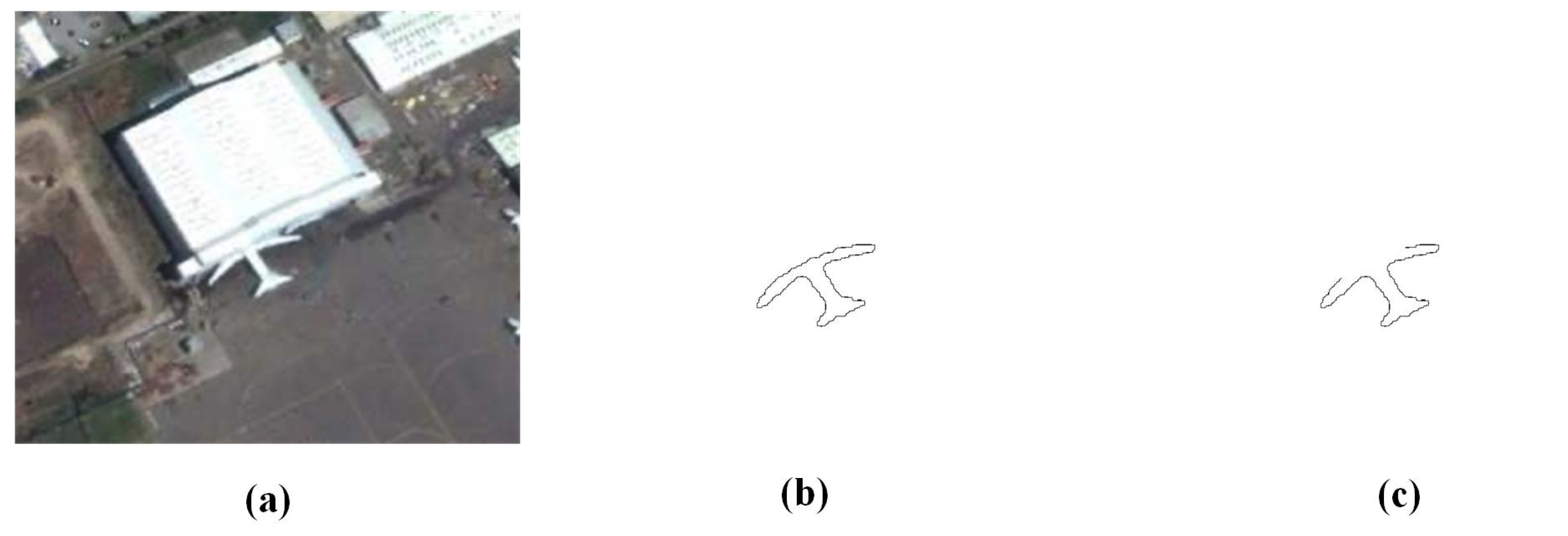
Shape descriptors are generally divided into global and local descriptors. Because shape description methods need to satisfy three invariances (translation invariance, scale shrinkage invariance, and rotation invariance), and it is difficult for local shape descriptors to ensure these three invariances, most of the existing shape description methods are based on the global feature of the target. For example, CCD (centroid contour distance) [17], FD-CCD (FD-based CCD) [18], FPD (farthest point distance) [19], SC (shape context) [20], IDSC (shape context based on inner distance) [21], AICD (affine-invariant curve descriptor) [22]. There have also been efficient global shape description methods in recent years, such as CBW (chord bunch balks) proposed by Bin Wang et al. in 2019 [23,24], and TCDs (triangular centroid distances) proposed by Chengzhuan Yang et al. in 2017 [25]. Remote sensing targets could be occluded, such as shown in Figure 1a, where the shape contour of the plane target in the remote sensing image is occluded. In this case, the obtained shape will be a severely deformed shape contour or a missing shape contour, as shown in Figure 1b,c. If the above global shape description method is still used, the recognition accuracy will be greatly reduced and the practical application ability of the target recognition method will be reduced. At this time, in order to correctly identify the target through shape, it is necessary to obtain the local shape features to describe the target. Therefore, for the occluded remote sensing target, the local shape description method will play an extremely important role, and the study of the local shape description method is of great value for the occluded target.

Figure 1.
(a) The original image of the occluded aircraft target acquired by the remote sensing vision system, (b) the deformed contour obtained after the aircraft contour extraction, and (c) the missing local contour obtained after the aircraft contour extraction. As can be seen from the picture, the extracted target contours are not complete.
However, existing local shape description methods, such as dynamic space warping (DSW) proposed by N. Alajlan et al. [26] and contour convexities and concavities (CCC) proposed by T. Adamek et al. [27], mostly due to considering three invariances and increasing the calculation amount (and, thus, increasing the recognition time cost), means they cannot be applied. Therefore, it is critical to research a fast and accurate local shape recognition method for the occluded target. A fast local shape description method based on feature richness, aimed at the local shape features of occluded targets, is proposed by using walking MBRs, where feature richness includes pixel richness, direction richness, and distance richness. It provides some theoretical support for the practical application of occluded remote sensing targets. The authors’ contributions include:
(1) A feature richness principle of the walking MBRs for the local shape contour of the occluded remote sensing target is proposed, which satisfies three invariances of shape recognition;
(2) Proposed local contour pixel richness feature based on the feature principle;
(3) Proposed local contour orientation richness feature based on the feature principle;
(4) Proposed local contour distance richness feature based on the feature principle;
(5) A fast shape local strong feature description method based on the constraint reduction of the feature structure is proposed for the remote sensing occluded target.
Detailed explanations and procedures of the proposed method are provided in the following sections. The second section presents a detailed introduction to the proposed method of FEW. The third section presents the calculation complexity analysis. The fourth section presents the performance and test results of the method, including a self-built small remote sensing target dataset and three internationally used shape datasets. The fifth section presents a discussion of the proposed method. The last section presents the conclusion.
2. The Proposed Method
In this paper, a shape recognition method based on the feature richness of local contour using walking MBRs is proposed for partially occluded remote sensing targets. Firstly, a certain length of the target contour is fixed from a certain contour point to obtain its MBR, and then the feature richness of the inner contour of the MBR is calculated, including the contour pixel richness, contour orientation richness, and contour distance richness. Finally, the minimum feature richness and maximum feature richness of the local contour are obtained as the target shape features, which form the local feature of the target shape. The structural framework of the proposed method is shown in Figure 2 below, and the algorithm framework is shown in Algorithm 1 in Table below.

Figure 2.
The structural framework of the proposed method is divided into seven parts, from the input of the occluded shape to the final output of shape recognition results using FEW.
The proposed method can be divided into six parts, from the input shape contour to the output shape recognition result, representing the complete step of shape recognition. See Section 3 for a detailed comparison and evaluation.
| Algorithm 1 |
| Input: Shape contour sampling points, ; |
| Output: Shape recognition similarity of constraint reduction, ; |
| 1: Create some sets of , |
| 2: represents the number of MBR; |
| 3: for each , do |
| 4: Calculate the walking MBR of the local contour from to a fixed length; |
| 5: for each , do; |
| 6: Calculate contour pixel richness , contour direction richness , and contour distance richness of contour ; |
| 7: Calculate feature richness, of , ; |
| 8: end for |
| 9: end for |
| 10: The feature richness of the shape is ; |
| 11: Calculate the maximum feature richness and the minimum feature richness ; |
| 12: Reduce restraint for to obtain the strong feature-richness ; |
| 13: Then, do shape matching and shape recognition to obtain recognition accuracy. |
| 14: Return |
2.1. New Concepts
Feature richness: Feature is an important weapon for the computer to describe remote sensing targets. The richer the feature of the target shape, the more easily the target shape can be recognized and perceived by the computer. Feature richness is defined as the information richness of features used by the computer to describe the target shape, also known as feature information strength.
Contour pixel richness: Pixels are important information for a computer to describe images, which is also a kind of feature of target shape contour because the shape contour in the image is accumulated from pixels with different parameters. Contour pixel richness is defined as the ratio of the number of pixels on a certain contour in a given area (in this paper the area is whole sides of MBR) when the recognition system describes the target. The larger the ratio of the number of contour pixels to four sides pixels, the greater the pixel richness of the contour.
Contour orientation richness: Orientation is an important feature for the computer to describe the image. Contour orientation richness is defined as the change of relative position between points on the contour, which is expressed as the average directional change in this paper. The greater the change, the greater the contour directional richness.
Contour distance richness: Distance is an important feature for the computer to describe target parameters in target image, especially in the points of shape contour. Contour distance richness is defined as the distribution of the distance between a contour and a given endpoint when a recognition system describes a target shape. The wider the distance distribution, the greater the distance richness of the contour.
Feature structure reduction constraint: Shape recognition is the recognition of shape features. The feature structure reduction constraint is defined as the factor that reduces the performance of shape recognition after obtaining shape features. In this paper, the constraints of structural features are expressed as reducing the weak features in the feature structures and leaving only strong features (minimum feature richness and maximum feature richness).
2.2. Local Contour MBR
The MBR refers to the maximum rectangular range of multiple two-dimensional shape (such as points, lines, and polygons) represented by two-dimensional coordinates. It is the rectangle whose boundary is determined by the maximum abscissa, minimum abscissa, maximum ordinate, and minimum ordinate of each vertex of a given shape. Such a rectangle contains a given image and has a minimum area, etc. The MBR can reflect the feature information of the target, such as direction, size, and position, and the structure with the feature information of the target can be used to describe the target, so the MBR can be used as one of the target features [28,29].
In general, there are two types of MBR: minimum area rectangle and minimum perimeter rectangle. In this article, the minimum area rectangle is used. The following steps are the key steps to calculating the MBR [28].
Step 1: Find the maximum and minimum points of the abscissa and ordinate of the shape contour points respectively;
Step 2: Use these four points to construct four tangents to the shape;
Step 3: If one or two lines coincide with an edge, calculate the area of the rectangle determined by the four lines and save it as the current minimum value. Otherwise, the current minimum value is defined as infinity;
Step 4: Rotate the lines clockwise until one of them coincides with the edge of the polygon;
Step 5: Calculate the area of the new rectangle and compare it with the current minimum area. If it is less than that, update and save the area of the new rectangle as the minimum area;
Step 6: Repeat steps 4 and 5 until the angle of the line is rotated more than 90 degrees;
Step 7: Obtain the MBR.
Figure 3 shows the MBRs of some local contours of the target shape.
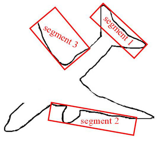
Figure 3.
The partial contour of an occluded remote sensing aircraft target is shown in the figure. For the specified contour segment 1, segment 2, and segment 3, the red rectangle is the MBR of its contour.
The set of contour points , denotes the number of contour points of the contour, and all the contours in this article are extracted by the Canny operator. The MBR of the contour obtained at this time can be expressed as Equation (1). This is also the basic criterion of the feature richness method proposed in this paper.
where, represent constants, represent -axis coordinates of the four vertices of the of the contour, respectively.
Assuming that the set of a certain contour segment is , and the inner region of the minimum outer rectangle of the contour segment is , then is obtained.
2.3. Contour Pixel Richness
Contour pixel refers to the number of pixels contained in a certain contour, which can represent the contour feature [30]. In this paper, contour pixel richness is expressed as the proportion of the number of contour pixels in the whole sides under the principle. Let the number of pixels on the contour segment be , and the number of pixels contained in the whole sides of the MBR of the contour be , then the calculation equation of the contour pixel richness is shown in Equation , and the calculation result is a constant.
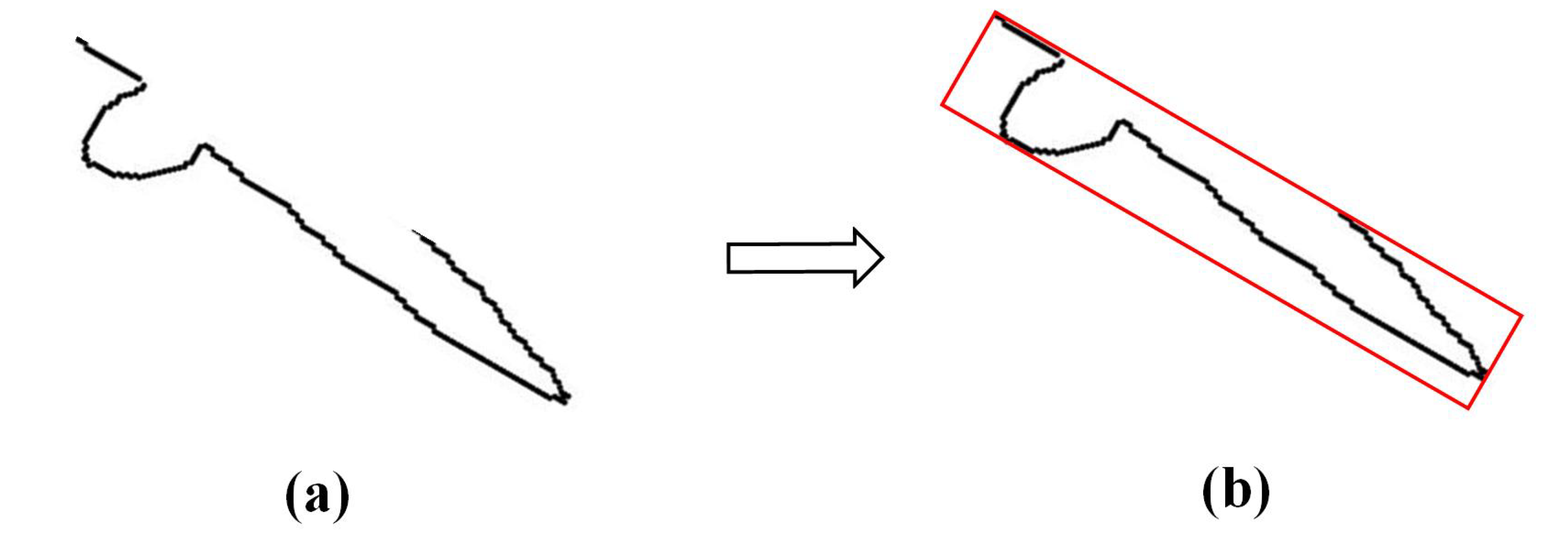
In Figure 4 below, (a) a specified contour of the aircraft, and (b) the MBR of the contour. After the calculation, the contour pixel richness of this contour segment is 0.52.

Figure 4.
The black line as shown in (a) the partial contour of a remote sensing aircraft target, and the red rectangle in (b) the pixel of the MBR’s four sides. The pixel richness of the contour can be obtained according to the number of pixels of the black line and the pixels of the entire rectangular sides.
2.4. Contour Orientation Richness
Contour orientation richness is defined as the intensity of position variation between contour points. In this paper, the contour orientation is obtained by coding. The chain code is a method to describe the orientation of a curve with the coordinates of the starting point of the curve and the direction code of the contour point. It is often used in image processing, computer graphics, pattern recognition, and other fields to represent the image feature [31,32]. Chain codes are generally divided into original chain codes, differential chain codes, and normalized chain codes.
2.4.1. Original Chain Code
Starting from a certain starting point of the boundary (curve or line), calculate the orientation of each line segment in a certain orientation, and express it with the corresponding pointing symbol of the fixed number of orientations. The result will form a digital sequence representing the boundary (curve or line), which is called the original chain code. The original chain code has translation invariance (the pointer is not changed during translation), but when the starting point S is changed, different chain code representations will be obtained, i.e., there is no uniqueness.
2.4.2. Differential Chain Code
The differential chain code denotes the coding of a dataset M, except for the first element , in which each element is represented as the difference between the current element and the previous element. Similar to the original chain code, the differential code page has translation invariance and scale invariance. The calculation formula of the “difference” code is shown in Equation (3).
Here, N represents the total number of directions encoded, and is the value of each sequence in the original chain code.
2.4.3. Normalized Differential Chain Code
The normalized chain code is to obtain the original chain code from any starting point for the closed boundary. The chain code is regarded as the N-bit natural number formed by the numbers in each direction, and the code is recycled in one direction to minimize the N-bit natural number formed by it. At this time, the chain code with a unique starting point is formed, which is called the normalized chain code. Simply speaking, it is to cycle the original chain code in one direction to minimize the N-bit natural number formed by it. Normalized differential chain codes have translation invariance, rotation invariance, and uniqueness. The acquisition method is: normalize the difference code. The calculation formula of the normalized differential chain code is shown in Equation (4) below.
where, the value of is the number of differential codes, and is the value of each sequence in the differential chain code, which can be "recursed" step by step in one orientation starting from any code value in the differential code. Based on the feature requirements of shape recognition, the shape representation method should satisfy three invariances. Considering the three coding methods and the uniqueness of the coding results, it is found that the normalized differential chain code can meet the requirements of shape descriptor for shape recognition, and it has translation, scale transformation, and rotation invariances. Therefore, it can be used as a feature vector to describe the shape contour.
2.4.4. 20-Chain Code Coding
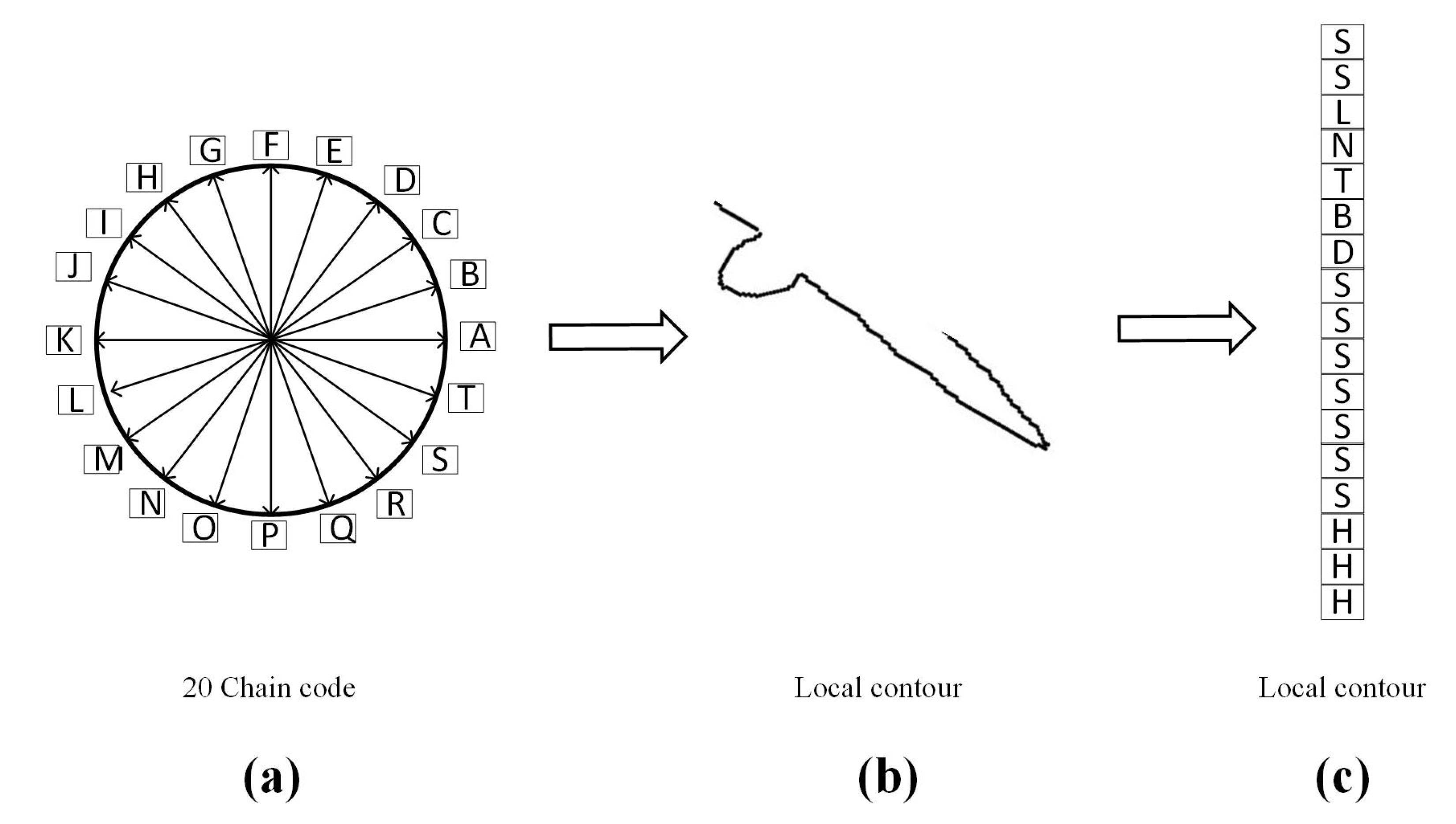
The connectivity orientation diagram of the 20-chain code designed in this method is shown in Figure 5a below. The 20 orientations corresponding to the current contour are divided into 20 regions respectively. According to the relative direction rule of the current contour point, , and the fourth contour point, , the position of each possible next direction is represented by letters from A to T. In the calculation process, the 20 orientations correspond to the natural numbers 0–19, respectively. The starting orientation was set as the right orientation of the image, and the starting point of the coding was the contour closest to the top left of the contour part. All the contours on the shape were coded in the clockwise orientation according to the above rules, so the initial contour was returned. Finally, the orientation feature of the contour is represented by the relative position relationship of all orientations of the contour. In Figure 5b is the local contour of a target, and (c) the orientation code of the contour obtained by coding according to the above rules.

Figure 5.
(a) The specified 20-orientation coding diagram, which contains 20-orientational code values, corresponding to the letters A–T. (b) a local contour, and (c) the code values of the contour in (b) after coding according to the specified coding rules (from top to bottom).
Contour orientation richness represents the intensity of variation of contour orientation, in other words, it is all the variation between the code value of the next direction and the current direction. For the whole local contour, it is expressed as the ratio of all variation to the number of the changes. In this method, the average variation of orientation is chosen as the contour orientation richness. Let the code values of all orientations on the contour be , where represents the number of codes on the contour, then the contour orientation richness can be calculated by the following Equation (5). The result is also a constant.
2.5. Contour Distance Richness
Distance is an important feature of an image [20,21,33]. Contour distance richness refers to the distance between the points on the contour and the long side and short side of the MBR according the principle, and two pairs of distance values on the long side and short side of the MBR can be obtained respectively. The minimum values of the two pairs of distances are respectively found as the distance of the point with respect to the MBR. Since the sum of these two pairs of values corresponds to the value of the perimeter of the MBR, the shortest distance and the longest distance selected here are the same. In this method, the minimum value is selected as the final distance of this point.
Assume a point on the contour, and find the distance between the long side and the short side of the MBR as . The minimum distance to the long side is , and the minimum distance to the short side is , the ultimate distance ’value ’ is expressed as . In this case, after the distance values of all contour points are obtained according to this rule, a vector set containing distances will be obtained, denoted as . The distance set is divided into bins according to the distance distribution, and a new vector set is obtained, which is defined as the contour distance richness under the , where the value of in this method is 10. Then the contour distance richness is expressed as the following Equation (6). This vector is also a constant vector.
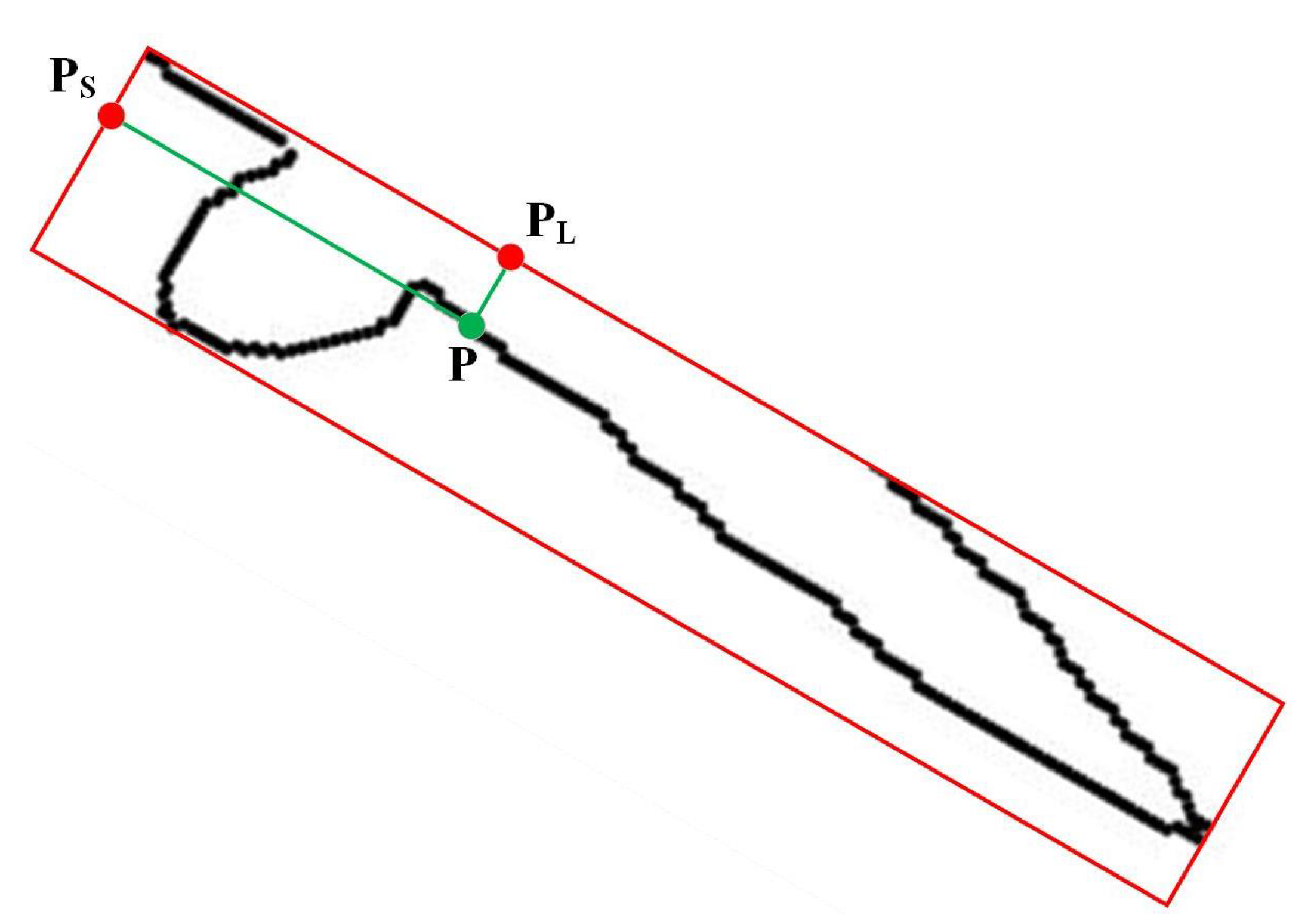
Figure 6 below shows a schematic diagram of a contour and its . Where, the green point P is the point on the contour, the red rectangle is the of the contour, and the red points and are the vertical points of P on the short and long sides of the , respectively. The green line · segments and are the shortest distances of P with respect to the short and long sides of the , respectively. According to the above rules, the minimum distance of the contour point with respect to the MBR can be obtained. After finding the minimum distance of all contour points, the minimum distance set of all points can be obtained.
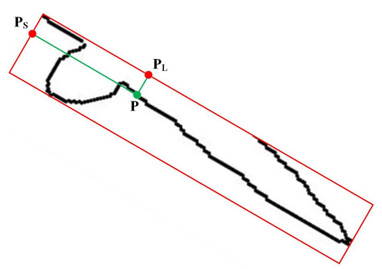
Figure 6.
The picture shows the minimum distance of contour point with respect to the MBR. According to this rule, the minimum distance set of all points on the contour can be obtained, and finally the distance richness of the contour can be obtained. Where, the red box denotes the MBR of the contour, and the green line segments denote the distance between a point on the contour and two rectangular sides.
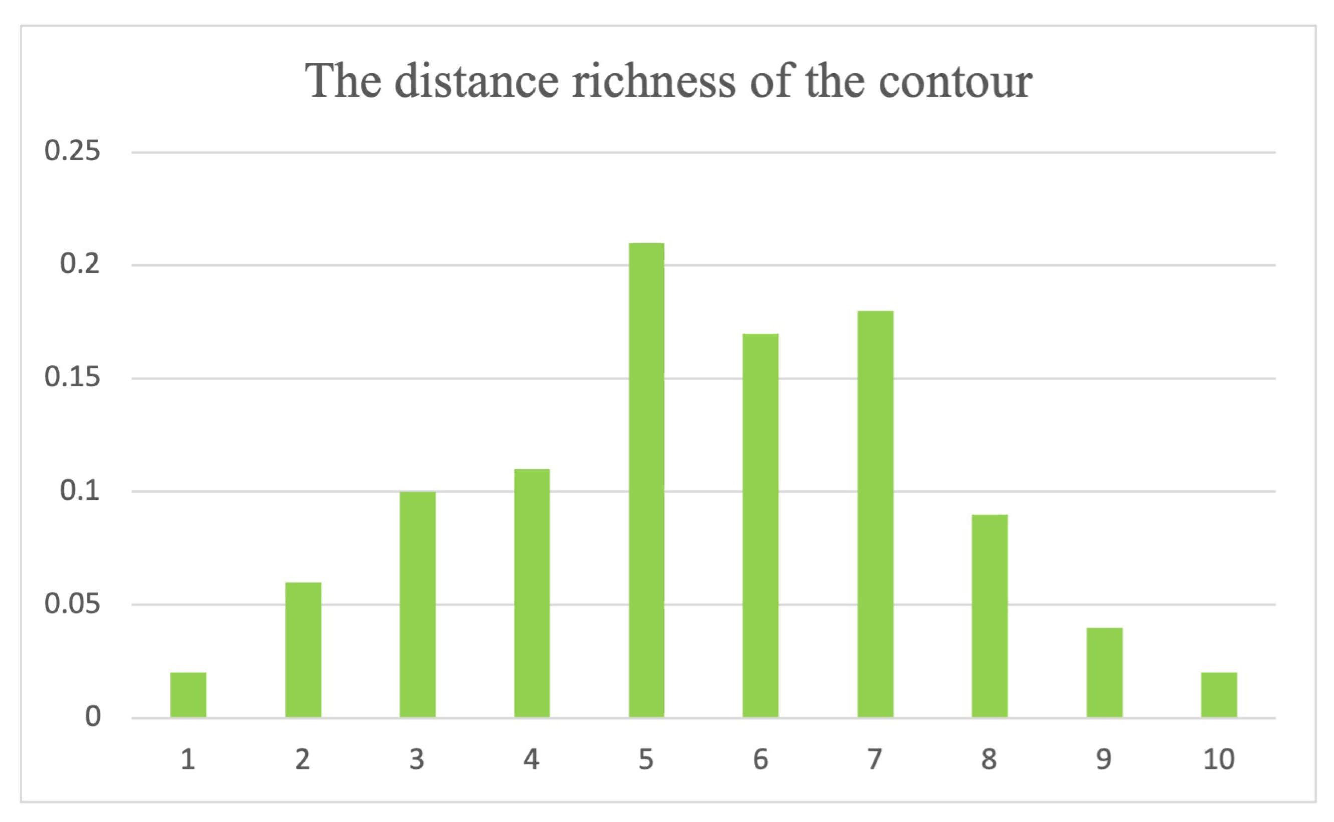
The histogram is widely used to represent the distribution features of the image [34,35,36]. In this method, the histogram is also used to represent the distance distribution vector of the contour. For the contour shown in Figure 6, the distance distribution obtained is shown in Figure 7 below.

Figure 7.
This histogram shows the distance distribution of the local contour in the MBR, which is also the specific representation of the contour distance richness.
2.6. Feature Richness for Walking MBRs
The method proposed in this paper is based on the local feature of the occluded contour. In order to describe the shape contour features of the occluded target more effectively, the authors use the principle of walking MBR to obtain the contour feature richness of the entire occluded target shape. The walking principle is: from the first point of the occluded contour, respectively, according to a certain number interval and a certain number points N to calculate all the MBRs. Then, the feature richness of each fixed-length contour to the MBR is calculated respectively, until the feature richness of the last contour with length N is obtained. Figure 8 below shows the walking diagram of the MBR to the occluded target contour. In Figure 8a, there is an occluded aircraft contour. On this contour, the MBR of the local contour is obtained from the upper left corner according to the principles described above, as shown in the red, green, yellow, and brown rectangles. The order of selection is counterclockwise, as shown by the fluorescent green circular arrow in (a). The walking principle of the MBR is shown in Figure 8b (the dashed box area in Figure 8a). The direction pointed by the fluorescent blue dashed arrow is the walking direction of the MBR, also known as the walking principle.
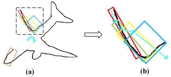
Figure 8.
(a) The design principles of the MBR for the occluded contour of the target; (b) the content of the dashed box in Figure (a) and the detailed walking principles of the MBR, as shown by the fluorescent blue arrow in Figure (b).
Based on the above walking principles of MBR, the MBR of all local contours and the corresponding feature richness can be obtained. At this time, according to the aforementioned solving methods of richness and the walking principles of the MBR, the pixel richness, orientation richness, and distance richness of the entire occluded target contour can be calculated according to the corresponding equations. The following Equation (7) represents the pixel richness of the entire occluded target contour, Equation (8) represents the directional richness of the entire occluded target contour, and Equation (9) represents the distance richness of the entire occluded target contour, where, represents the number of local contour segments of the entire occluded target and the number of minimum enclosing rectangles. indicates the number of bins.
According to the above three equations, the feature richness of the entire occluded target contour can be calculated and expressed as the following Formula (10).
In order to reduce the complexity of the feature structure of the shape contour, this method uses the concept of constraint reduction to select strong features as the final occluded target contour features, including the maximum contour richness and the minimum contour richness. As we all know, strong features are more suitable to describe target features and distinguish different targets more easily. The maximum and minimum contour richness are expressed in Equations (11) and (12), respectively.
Then, the feature richness , which is finally used to represent the occluded contour, can be obtained and expressed as the following Equation (13).
2.7. Feature Matching
The feature matching stage is the process of similarity matching after obtaining the final shape feature, which is also an important step after feature extraction. According to the sections described above, the feature richness of the occluded target contour can be obtained, and feature matching can be carried out after the feature vector is obtained. Based on the feature structure of the occluded shape in this method, the Euclidean distance is used to measure the shape similarity, and then the feature matching is carried out and the recognition result is obtained. In order to ensure the integrity of the feature vectors, the difference between the maximum and the minimum feature richness is calculated as the basis for the similarity measurement of the two shapes. The specific matching equation can be expressed as the following Equation (14).
3. Complexity
The complexity of shape recognition refers to the complexity of the shape description method in the process of feature computation. The feature richness description method based on walking MBR adopted in this paper is itself a computational process with low computational complexity, because the calculation results including contour pixel richness, contour orientation richness and contour distance richness are all one-dimensional constant vectors. In addition, in this paper, the feature structure is finally reduced by the constraint reduction (only the strong features are selected for recognition and matching, in other words, they are the maximum feature richness and the minimum feature richness), which greatly reduces the matching cost, so the proposed method has low computational complexity. When the number of contour points of the input shape contour is and the minimum peripheral rectangle is calculated according to each point, the complexity of the method in this paper is lower than that of some well-known shape description methods. Although the proposed method also processes all the contour points of the occluding object, the feature structure reduction constraint is added in the feature matching stage and the final total complexity is . This also becomes an important basis for this method to improve recognition speed. The computational complexity of several representative shape description methods is listed in the following Table 1. Since , the proposed method has the lowest complexity.

Table 1.
Some representative shape recognition methods feature computational complexities.
4. Performance on the Four Datasets
In order to evaluate the performance of the proposed shape recognition method, the shape features formed by the proposed method are verified in a self-built remote sensing target dataset and three mainstream international shape recognition datasets. The shape contours of the two mainstream shape datasets (MPEG-7 Part B and Plant Leaf 270) are complete and cannot verify the accuracy of the occluded target shape recognition in this paper, so the current shape is artificially added with partial occlusion every time the shape matching is performed. These four datasets include the FEW 100 dataset, the MPEG-7 Part B dataset, the Plant Leaf 270 dataset, and the Kimia 99 dataset. There are different types of 2D shapes in the datasets, which can be used as validation datasets for the speed and accuracy of shape recognition. Moreover, the shape images on these datasets are all noiseless and will not affect the shape recognition results. Therefore, the contour extracted in the article will not be affected by noise. In the experiment of this paper, all the methods used for comparison are written with MATLAB software. It runs on macOS 11 PCS with Intel(R) Core (TM)(America) i7-4850 2.30 GHz CPU and 8 gb DDR3 DRAM.
4.1. Performance on FEW 100
The FEW 100 dataset consists of 100 remote sensing target shapes collected by the authors from the internet and some remote sensing target databases (VEDAI, OIRDS, and RSOD). The dataset has 5 categories (aircraft, ship, storeroom, helicopter, oil tank), and each category has 20 shapes. When shape recognition is performed on this dataset, a part of occlusion is artificially added to each identified target, and then it is matched with the complete target contour in the whole dataset. In Figure 9, the left-most column is the shape of the occluded, and the rest are the complete shape of remote sensing target. Among them, all shapes in the dataset are processed from color remote sensing images, which makes it easier to distinguish the shapes of the targets.
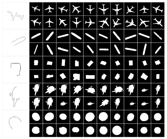
Figure 9.
The leftmost column is a schematic diagram of the target shapes artificially occluded (to verify the effectiveness of the proposed method in the shape recognition stage), and the remaining part is 100 single remote sensing target shapes collected from the internet and remote sensing image databases.
All shapes in this dataset are recognized according to the method proposed in this paper. The experimental results are shown in Table 2 below, which also contains the results of some other classical shape recognition methods. Among them, AICD [22] is a shape recognition method specifically for occluded shapes, proposed by Huijing Fu et al. Although this method has good performance, it is not as effective as the method proposed in this paper. It is obvious that the proposed method has the most efficient recognition performance, including higher recognition accuracy and faster recognition speed.

Table 2.
Comparison of performance on FEW 100 dataset.
4.2. Performance on Mpeg-7 Part B
The MPEG-7 Part B dataset is often used by scholars to test the performance of shape recognition methods, and the results of many articles are based on this dataset [40,41,42,43,44]. There are 70 types of shapes in this dataset, and each type has 20 different shapes, a total of 1400 shapes. Compared with other shape datasets, this dataset has more and richer shapes, which is of great significance to the performance of shape recognition. Figure 10 shows a portion of the shape in this dataset, and this section shows the test results of the method. Since the shape contours in this dataset are all complete, in order to better illustrate the recognition effectiveness of the proposed method for occluded target shapes, each shape to be recognized is artificially occluded, as shown in the first column of Figure 10. Table 3 below shows the performance of the proposed FEW and other state-of-the-art descriptors.
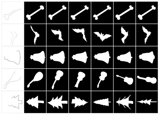
Figure 10.
The leftmost column is a schematic diagram of the object shape contour artificially occluded (to verify the effectiveness of the proposed method in the shape recognition stage), and the rest is part of the shapes in MPEG-7 Part B.

Table 3.
Comparison of the bull’s eyes test score and matching time on MPEG-7 Part B dataset.
4.3. Performance on Plant Leaf 270
The Plant Leaf 270 dataset is a leaf shape dataset. There are 270 leaves in this dataset (30 classes, each containing 9 leaves). This dataset is also an important validation dataset in the shape recognition method. Similar to the above two datasets, each shape to be recognized is occluded in the shape recognition stage. Some of the shapes in this database are shown in Figure 11.
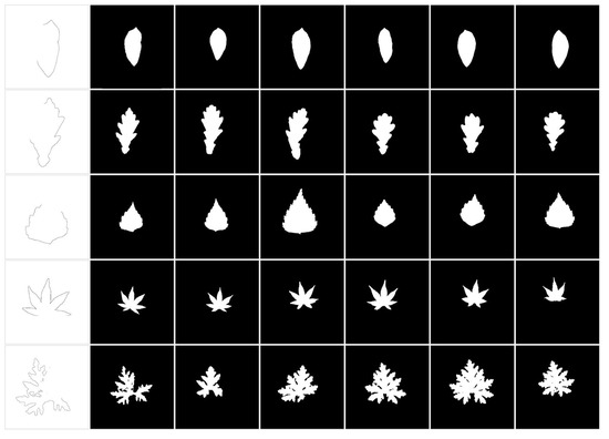
Figure 11.
The left-most column shows a schematic diagram of the object shape contour artificially occluded (in order to verify the effectiveness of the proposed method in the shape recognition stage), and the rest are the five types of shapes in the Plant Leaf 270.
In the recognition accuracy evaluation of this dataset, the K-nearest neighbor leave-one method is adopted. Find K shapes with the highest similarity to each shape (except itself), and mark the category of this shape as the category with the highest frequency among K shapes. Finally count all the times of successful recognition, so as to obtain the overall recognition accuracy. The experimental results of some classical shape description methods tested in this dataset are shown in Table 4. It is obvious that the proposed method has the best recognition performance.

Table 4.
Accuracy rate and matching time of our descriptor and some other descriptors on the Swedish plant leaf.
4.4. Performance on Kimia 99
Kimia 99 is also an internationally available shape dataset. Several articles have used Kimia 99 as a method validation dataset. It has a total of 99 shapes, which are divided into 9 categories, each with 11 different shapes. Although the volume of this dataset is small, there are a large number of occluded or partially incomplete shapes in this dataset, which is very suitable for the occlusion target shape recognition method in this paper. Therefore, the shapes to be recognized in this dataset do not need artificial occlusion and can be directly recognized. The shape contours of all the shapes in the dataset are shown in Figure 12.
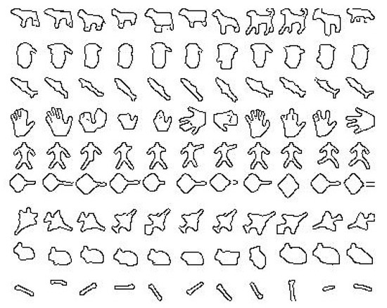
Figure 12.
Example of shapes in the Kim99 dataset. One object for each one of the nine categories is shown.
The recognition strategy of this dataset is: each shape is successively set as the shape to be recognized, and then a similar shape is recognized among the remaining shapes. In the recognition results, the correct number of collisions from the first most similar shape to the tenth most similar shape of each shape to be recognized is calculated, and the final statistical results are used to evaluate the recognition performance of the proposed method. The test results of some representative shape description methods tested in this dataset are shown in Table 5, including our description method. It can be seen from the experimental results that the proposed method still has higher accuracy and fewer matching time on Kimia 99 dataset.

Table 5.
Comparison of correct hit-rate and matching time on Kimia 99 dataset.
4.5. Comparison of Artificial Occlusion and Non-Occlusion Results
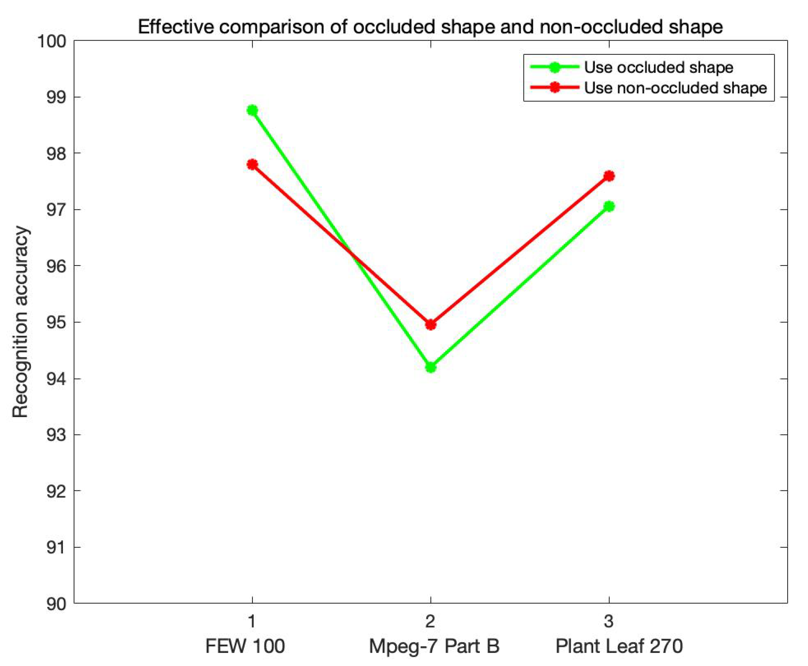
As the tests on datasets FEW 100, MPEG-7 Part B, and Plant Leaf 270 were meant the shape recognition methods for the occluded targets proposed in this paper, each shape to be recognized was artificially occluded. In order to better verify the effectiveness of the proposed method, an additional shape recognition test on the original dataset was carried out. On the basis of not occluding the shape to be recognized, the method proposed in this paper is used for shape recognition. The recognition results of the occluded shape and non-occluded shape in the three datasets are respectively represented by the line diagram in Figure 13 below. Although the recognition result of the proposed method for non-occluded shapes is better, it is still higher than other recognition methods for non-occluded shapes in the table. In addition, when occlusion is added artificially, the recognition accuracies of other shape recognition methods decrease significantly [47], but the method proposed in this paper almost keeps the same recognition accuracy.
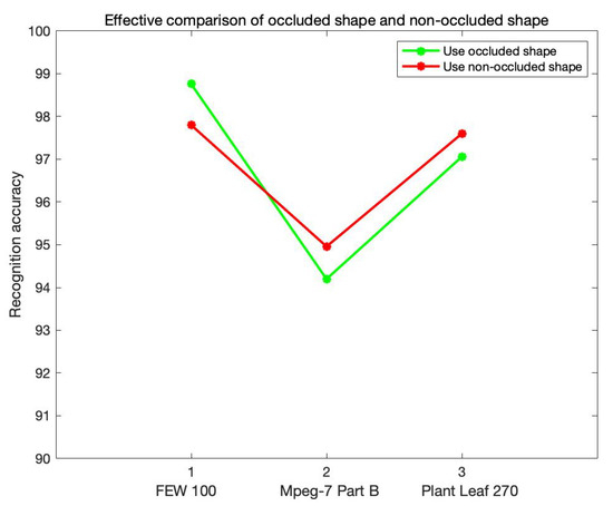
Figure 13.
The comparison between occluded shape recognition and non-occluded shape recognition on three datasets, where the green polyline denotes the result of recognition after artificial occlusion, and the red polyline denotes the result of shape recognition without occlusion. It can be seen that the proposed method is still sophisticated for non-occluded shape recognition, and shows high recognition performance.
4.6. Comparison of Results with Different Degrees of Occlusion
It is well known that different degrees of artificial occlusion have a serious impact on the recognition of the occluded shape. In the above experiments, 0–1/4 random occlusion is performed on the shapes of three datasets (FEW 100, MPEG-7 Part B, and Plant Leaf 270), which has the best performance compared with other state-of-the-art shape recognition methods. In order to illustrate the influence of different degrees of occlusion on the shape recognition method and the high performance of the proposed method, comparative experiments with different degrees of occlusion are conducted in this section. Different random occlusions of 0–1/4, 1/4–1/2, 1/2–3/4, and 3/4–1 were performed on the FEW 100 datasets (The results on other datasets are similar), and the obtained shape recognition accuracies and the accuracies of some well-known shape recognition methods are shown in Table 6 below. According to the experimental results, it is obvious that the shape recognition accuracy decreases gradually with the increase of the occlusion degree, which is also an inevitable result because the larger degree of occlusion will cause the loss of the feature information of the shape. Nevertheless, no matter what degree of artificial occlusion, the proposed method has higher recognition accuracy, which further demonstrates the excellent performance of the proposed method.

Table 6.
Comparison of different degrees of occlusion.
5. Discussion
In this paper, a method of shape recognition for occluded remote sensing targets is proposed by using the local contour strong feature richness to the walking MBR. The feature richness of shape contour includes contour pixel richness, contour orientation richness, and contour distance richness. The larger the richness of the contour, the more feature information the contour contains (and the easier the shape to be recognized is). The walking MBR is for the contour of fixed length and walks on the whole occluded shape contour in a clockwise direction. The MBR itself can represent the direction, size, position, and other features of a local contour, which is very suitable for describing shape features. It is worth mentioning that in the last stage of feature structure, the strategy of constraint reduction is used to reduce the weak feature constraints of feature structure, and only the strong feature of shape is used to describe the shape, which will greatly reduce the matching time of shape recognition and improve the speed of shape recognition. Since there is no shape dataset about occluded remote sensing targets at present, in order to verify the efficiency of the proposed method, the validation is carried out on a self-built remote sensing target shape dataset and three international common datasets respectively. Among them, the first three shape datasets all conduct artificial partial occlusion of the recognized target shape, in order to better illustrate the effectiveness of the proposed method for occluded remote sensing target recognition. The last dataset is occluded due to its large deformation, so no artificial occlusion is added. The recognition speed on these four datasets is all lower than 1 ms, and the recognition accuracy is significantly improved compared with other state-of-the-art and well-known shape descriptors. The recognition result on the self-built occlusion remote sensing target is even close to 100%, which provides strong theoretical support for the recognition application of the occluded remote sensing target. In Section 4.5 and Section 4.6, comparative experiments also better validate the efficiency of the proposed method, which has sophisticated performance for both occluded target shapes and non-occluded target shapes.
In addition, readers may doubt that the external environment will have an impact on the quality of the acquired target shape image in the contour extraction stage. However, before the object recognition stage, there must be the object detection stage; these are two completely different stages. In the stage of object detection, it is necessary to consider the influence of external factors on the object image, but in the stage of object shape recognition, the shape image that can be recognized by the computer has been acquired by default in the stage of object detection, so it is not necessary to consider the influence of the external environment of the target on the shape recognition. Finally, in future research, we will continue to study the shape recognition of occluded objects, build a large dataset specifically for occluded remote sensing target shape recognition, and publish relevant papers.
Moreover, it can be seen from this article that the proposed shape features are in the spatial domain rather than in the frequency domain and the images in the datasets used in this article do not have noise themselves, so it is not necessary to consider the impact of noise on the recognition results. Finally, even if there is noise in the image, the noise will affect all shape recognition methods, but our proposed method still has the best performance, which again proves the effectiveness of the proposed method for remote sensing target shape recognition.
6. Conclusions
FEW is a shape recognition method with low computational costs, high recognition efficiency, and strong robustness. In this method, shape recognition is performed for the occluded remote sensing target shape contour, and the final shape features are invariant to translation, rotation, and scale transformation. This method obtains the feature richness of the local contour in the MBR based on the walking MBRs, including contour pixel richness, contour orientation richness, and contour distance richness. The obtained feature richness is a one-dimensional constant vector, which greatly reduces the matching cost in the feature matching stage and makes the method have a faster recognition speed. In addition, the final occluded target shape feature structure is simplified into the recognition process of strong features (minimum richness and maximum richness) by the strategy of constraint reduction, which greatly reduces the complexity of the feature structure and accelerates the recognition speed. The final matching time is less than 1 ms. Since the occlusion remote sensing target shape dataset is difficult to obtain, this paper uses a self-built remote sensing target shape dataset and three general shape recognition datasets to verify the performance of the proposed method. It is worth mentioning that the authors of this paper artificially occluded the shapes to be recognized in both the self-built dataset and the two general datasets, in order to better verify the proposed method for occluded remote sensing target shape recognition. The experimental results demonstrate the sophisticated recognition performance of FEW. Compared with some state-of-the-art shape recognition methods, including those for occluded shapes, FEW not only guarantees higher recognition accuracy but also greatly enhances the recognition speed. The recognition speed of the proposed method is more than 1000 times faster than some other methods and the recognition accuracy is close to 100% in the self-built dataset, which greatly enhances the recognition speed of the occluded remote sensing target and provides a more powerful performance support for the practical application of the remote sensing target recognition.
Author Contributions
Z.L.: Conceptualization, methodology, software, validation, formal, analysis, investigation, resources, data curation, writing—original draft preparation, visualization; B.G.: conceptualization, supervision, project administration; F.M.: writing—review and editing. All authors have read and agreed to the published version of the manuscript.
Funding
This work was supported by the National Natural Science Foundation of China under grant 62171341 (corresponding author: Baolong Guo) and the Natural Science Basic Research Program of Shaanxi Province of China under grant 2020JM-196 (corresponding author: Fanjie Meng).
Data Availability Statement
Not applicable.
Acknowledgments
Thanks to the editors and reviewers for their contributions to this article.
Conflicts of Interest
The authors declare that they have no known competing financial interests or personal relationships that could have appeared to influence the work reported in this paper.
References
- Xu, S.; Wang, J.; Shou, W.; Ngo, T.; Sadick, A.M.; Wang, X. Computer vision techniques in construction: A critical review. Arch. Comput. Methods Eng. 2021, 28, 3383–3397. [Google Scholar] [CrossRef]
- Guo, M.H.; Xu, T.X.; Liu, J.J.; Liu, Z.N.; Jiang, P.T.; Mu, T.J.; Zhang, S.H.; Martin, R.R.; Cheng, M.M.; Hu, S.M. Attention mechanisms in computer vision: A survey. Comput. Vis. Media 2022, 8, 331–368. [Google Scholar] [CrossRef]
- Wu, Z.; Chen, Y.; Zhao, B.; Kang, X.; Ding, Y. Review of weed detection methods based on computer vision. Sensors 2021, 21, 3647. [Google Scholar] [CrossRef] [PubMed]
- Huang, W.; Li, G.; Chen, Q.; Ju, M.; Qu, J. CF2PN: A cross-scale feature fusion pyramid network based remote sensing target detection. Remote Sens. 2021, 13, 847. [Google Scholar] [CrossRef]
- Sun, Y.; Jiang, W.; Yang, J.; Li, W. SAR Target Recognition Using cGAN-Based SAR-to-Optical Image Translation. Remote Sens. 2022, 14, 1793. [Google Scholar] [CrossRef]
- Ismail, N.; Malik, O.A. Real-time visual inspection system for grading fruits using computer vision and deep learning techniques. Inf. Process. Agric. 2022, 9, 24–37. [Google Scholar] [CrossRef]
- Dong, C.; Liu, J.; Xu, F. Ship detection in optical remote sensing images based on saliency and a rotation-invariant descriptor. Remote Sens. 2018, 10, 400. [Google Scholar] [CrossRef]
- Pappas, O.; Achim, A.; Bull, D. Superpixel-level CFAR detectors for ship detection in SAR imagery. IEEE Geosci. Remote Sens. Lett. 2018, 15, 1397–1401. [Google Scholar] [CrossRef]
- Chen, F.; Ren, R.; Van de Voorde, T.; Xu, W.; Zhou, G.; Zhou, Y. Fast automatic airport detection in remote sensing images using convolutional neural networks. Remote Sens. 2018, 10, 443. [Google Scholar] [CrossRef]
- Xu, B.; Chen, Z.; Zhu, Q.; Ge, X.; Huang, S.; Zhang, Y.; Liu, T.; Wu, D. Geometrical Segmentation of Multi-Shape Point Clouds Based on Adaptive Shape Prediction and Hybrid Voting RANSAC. Remote Sens. 2022, 14, 2024. [Google Scholar] [CrossRef]
- Chen, P.; Zhou, H.; Li, Y.; Liu, B.; Liu, P. Shape similarity intersection-over-union loss hybrid model for detection of synthetic aperture radar small ship objects in complex scenes. IEEE J. Sel. Top. Appl. Earth Obs. Remote Sens. 2021, 14, 9518–9529. [Google Scholar] [CrossRef]
- Yang, X.; Li, S.; Sun, S.; Yan, J. Anti-Occlusion Infrared Aerial Target Recognition with Multi-Semantic Graph Skeleton Model. IEEE Trans. Geosci. Remote Sens. 2022, 60, 1–13. [Google Scholar]
- Bai, X.; Yang, X.; Latecki, L.J.; Liu, W.; Tu, Z. Learning context-sensitive shape similarity by graph transduction. IEEE Trans. Pattern Anal. Mach. Intell. 2009, 32, 861–874. [Google Scholar]
- Yang, X.; Koknar-Tezel, S.; Latecki, L.J. Locally constrained diffusion process on locally densified distance spaces with applications to shape retrieval. In Proceedings of the 2009 IEEE Conference on Computer Vision and Pattern Recognition, Miami, FL, USA, 20–25 June 2009; IEEE: Piscatawy, NJ, USA, 2009; pp. 357–364. [Google Scholar]
- Bai, X.; Wang, B.; Yao, C.; Liu, W.; Tu, Z. Co-transduction for shape retrieval. IEEE Trans. Image Process. 2011, 21, 2747–2757. [Google Scholar]
- Kontschieder, P.; Donoser, M.; Bischof, H. Beyond pairwise shape similarity analysis. In Proceedings of the Asian Conference on Computer Vision, Xi’an, China, 23–27 September 2009; Springer: Berlin/Heidelberg, Germany, 2009; pp. 655–666. [Google Scholar]
- Hasim, A.; Herdiyeni, Y.; Douady, S. Leaf shape recognition using centroid contour distance. In Proceedings of the IOP Conference Series: Earth and Environmental Science, Sanya, China, 21–23 November 2016; IOP Publishing: Bristol, UK, 2016; Volume 31, p. 012002. [Google Scholar]
- Zhang, D.; Lu, G. Study and evaluation of different Fourier methods for image retrieval. Image Vis. Comput. 2005, 23, 33–49. [Google Scholar] [CrossRef]
- El-ghazal, A.; Basir, O.; Belkasim, S. Farthest point distance: A new shape signature for Fourier descriptors. Signal Process. Image Commun. 2009, 24, 572–586. [Google Scholar] [CrossRef]
- Belongie, S.; Malik, J.; Puzicha, J. Shape matching and object recognition using shape contexts. IEEE Trans. Pattern Anal. Mach. Intell. 2002, 24, 509–522. [Google Scholar] [CrossRef]
- Ling, H.; Jacobs, D.W. Shape classification using the inner-distance. IEEE Trans. Pattern Anal. Mach. Intell. 2007, 29, 286–299. [Google Scholar] [CrossRef]
- Fu, H.; Tian, Z.; Ran, M.; Fan, M. Novel affine-invariant curve descriptor for curve matching and occluded object recognition. IET Comput. Vis. 2013, 7, 279–292. [Google Scholar] [CrossRef]
- Wang, B.; Gao, Y.; Sun, C.; Blumenstein, M.; La Salle, J. Chord Bunch Walks for Recognizing Naturally Self-Overlapped and Compound Leaves. IEEE Trans. Image Process. 2019, 28, 5963–5976. [Google Scholar] [CrossRef]
- Wang, B.; Gao, Y.; Sun, C.; Blumenstein, M.; La Salle, J. Can walking and measuring along chord bunches better describe leaf shapes? In Proceedings of the IEEE Conference on Computer Vision and Pattern Recognition 2017, Honolulu, HI, USA, 21–26 July 2017; pp. 6119–6128. [Google Scholar]
- Yang, C.; Wei, H.; Yu, Q. A novel method for 2D nonrigid partial shape matching. Neurocomputing 2018, 275, 1160–1176. [Google Scholar] [CrossRef]
- Alajlan, N.; El Rube, I.; Kamel, M.S.; Freeman, G. Shape retrieval using triangle-area representation and dynamic space warping. Pattern Recognit. 2007, 40, 1911–1920. [Google Scholar] [CrossRef]
- Bertamini, M.; Wagemans, J. Processing convexity and concavity along a 2-D contour: Figure–ground, structural shape, and attention. Psychon. Bull. Rev. 2013, 20, 191–207. [Google Scholar] [CrossRef] [PubMed]
- Li, Z.; Guo, B.; Ren, X.; Liao, N. Vertical Interior Distance Ratio to Minimum Bounding Rectangle of a Shape. In Proceedings of the International Conference on Hybrid Intelligent Systems, Virtual Event, 14–16 December 2020; Springer: Berlin/Heidelberg, Germany, 2020; pp. 1–10. [Google Scholar]
- Li, Z.; Guo, B.; He, F. A multi-angle shape descriptor with the distance ratio to vertical bounding rectangles. In Proceedings of the 2021 International Conference on Content-Based Multimedia Indexing (CBMI), Lille, France, 28–30 June 2021; IEEE: Piscataway, NJ, USA, 2021; pp. 1–4. [Google Scholar]
- Zhang, J.; Wenyin, L. A pixel-level statistical structural descriptor for shape measure and recognition. In Proceedings of the 2009 10th International Conference on Document Analysis and Recognition, Barcelona, Spain, 26–29 June 2009; IEEE: Piscataway, NJ, USA, 2009; pp. 386–390. [Google Scholar]
- Hassoon, I.M. Shape Feature Extraction Techniques for Fruits: A Review. Iraqi J. Sci. 2021, 62, 2425–2430. [Google Scholar] [CrossRef]
- Wu, D.; Zhang, C.; Ji, L.; Ran, R.; Wu, H.; Xu, Y. Forest Fire Recognition Based on Feature Extraction from Multi-View Images. Trait. Signal 2021, 38, 3. [Google Scholar] [CrossRef]
- Berretti, S.; Del Bimbo, A.; Pala, P. Retrieval by shape similarity with perceptual distance and effective indexing. IEEE Trans. Multimed. 2000, 2, 225–239. [Google Scholar]
- Albawendi, S.; Lotfi, A.; Powell, H.; Appiah, K. Video based fall detection using features of motion, shape and histogram. In Proceedings of the 11th Pervasive Technologies Related to Assistive Environments Conference, Corfu, Greece, 26–29 June 2018; pp. 529–536. [Google Scholar]
- Cho, S.I.; Kang, S.J. Histogram shape-based scene-change detection algorithm. IEEE Access 2019, 7, 27662–27667. [Google Scholar] [CrossRef]
- Fanfani, M.; Bellavia, F.; Iuliani, M.; Piva, A.; Colombo, C. FISH: Face intensity-shape histogram representation for automatic face splicing detection. J. Vis. Commun. Image Represent. 2019, 63, 102586. [Google Scholar] [CrossRef]
- Bicego, M.; Lovato, P. A bioinformatics approach to 2D shape classification. Comput. Vis. Image Underst. 2016, 145, 59–69. [Google Scholar] [CrossRef]
- Yang, X.; Bai, X.; Latecki, L.J.; Tu, Z. Improving shape retrieval by learning graph transduction. In Proceedings of the European Conference on Computer Vision, Marseille, France, 12–18 October 2008; Springer: Berlin/Heidelberg, Germany, 2008; pp. 788–801. [Google Scholar]
- Kaothanthong, N.; Chun, J.; Tokuyama, T. Distance interior ratio: A new shape signature for 2D shape retrieval. Pattern Recognit. Lett. 2016, 78, 14–21. [Google Scholar] [CrossRef]
- Yildirim, M.E. Quadrant-based contour features for accelerated shape retrieval system. J. Electr. Eng. 2022, 73, 197–202. [Google Scholar] [CrossRef]
- Sikora, T. The MPEG-7 visual standard for content description-an overview. IEEE Trans. Circuits Syst. Video Technol. 2001, 11, 696–702. [Google Scholar] [CrossRef]
- Coimbra, M.T.; Cunha, J.S. MPEG-7 visual descriptors—Contributions for automated feature extraction in capsule endoscopy. IEEE Trans. Circuits Syst. Video Technol. 2006, 16, 628–637. [Google Scholar] [CrossRef]
- Doulamis, N. Iterative motion estimation constrained by time and shape for detecting persons’ falls. In Proceedings of the 3rd International Conference on PErvasive Technologies Related to Assistive Environments, Petra, Greece, 23–25 June 2010; pp. 1–8. [Google Scholar]
- Ntalianis, K.S.; Doulamis, N.D.; Doulamis, A.D.; Kollias, S.D. A feature point based scheme for unsupervised video object segmentation in stereoscopic video sequences. In Proceedings of the 2000 IEEE International Conference on Multimedia and Expo, ICME2000, Proceedings Latest Advances in the Fast Changing World of Multimedia (Cat. No. 00TH8532), New York, NY, USA, 30 July–2 August 2000; IEEE: Piscatawy, NJ, USA, 2000; Volume 3, pp. 1543–1546. [Google Scholar]
- Hu, R.; Jia, W.; Ling, H.; Huang, D. Multiscale distance matrix for fast plant leaf recognition. IEEE Trans. Image Process. 2012, 21, 4667–4672. [Google Scholar] [PubMed]
- Yang, L.; Wang, L.; Zhang, Z.; Zhuang, J. Bag of feature with discriminative module for non-rigid shape retrieval. Digit. Signal Process. 2022, 120, 103240. [Google Scholar] [CrossRef]
- Li, Z.; Guo, B.; Meng, F. Fast Shape Recognition via the Restraint Reduction of Bone Point Segment. Symmetry 2022, 14, 1670. [Google Scholar] [CrossRef]
Publisher’s Note: MDPI stays neutral with regard to jurisdictional claims in published maps and institutional affiliations. |
© 2022 by the authors. Licensee MDPI, Basel, Switzerland. This article is an open access article distributed under the terms and conditions of the Creative Commons Attribution (CC BY) license (https://creativecommons.org/licenses/by/4.0/).

