Article

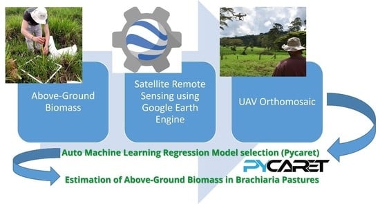
Predictive Modeling of Above-Ground Biomass in Brachiaria Pastures from Satellite and UAV Imagery Using Machine Learning Approaches

1
Grupo de Investigación Ambiental en el Desarrollo Sustentable GIADES, Carrera de Ingeniería Ambiental, Universidad Politécnica Salesiana, Quito 170702, Ecuador
2
International Center for Tropical Agriculture (CIAT), A.A. 6713, Cali 763537, Colombia
*
Author to whom correspondence should be addressed.
Remote Sens. 2022, 14(22), 5870; https://doi.org/10.3390/rs14225870
Submission received: 17 October 2022 / Revised: 16 November 2022 / Accepted: 17 November 2022 / Published: 19 November 2022

Abstract

:
Grassland pastures are crucial for the global food supply through their milk and meat production; hence, forage species monitoring is essential for cattle feed. Therefore, knowledge of pasture above-ground canopy features help understand the crop status. This paper finds how to construct machine learning models to predict above-ground canopy features in Brachiaria pasture from ground truth data (GTD) and remote sensing at larger (satellite data on the cloud) and smaller (unmanned aerial vehicles (UAV)) scales. First, we used above-ground biomass (AGB) data obtained from Brachiaria to evaluate the relationship between vegetation indices (VIs) with the dry matter (DM). Next, the performance of machine learning algorithms was used for predicting AGB based on VIs obtained from ground truth and satellite and UAV imagery. When comparing more than twenty-five machine learning models using an Auto Machine Learning Python API, the results show that the best algorithms were the Huber with R2 = 0.60, Linear with R2 = 0.54, and Extra Trees with R2 = 0.45 to large scales using satellite. On the other hand, short-scale best regressions are K Neighbors with an R2 of 0.76, Extra Trees with an R2 of 0.75, and Bayesian Ridge with an R2 of 0.70, demonstrating a high potential to predict AGB and DM. This study is the first prediction model approach that assesses the rotational grazing system and pasture above-ground canopy features to predict the quality and quantity of cattle feed to support pasture management in Colombia.

Graphical Abstract

1. Introduction

Grasslands, after forests, are the largest terrestrial carbon sink and cover 31.5% of the earth’s total landmass [1,2,3]. Grasslands are classified as natural (formed in natural climatic conditions), semi-natural (developed through human management), and improved grasslands (pastures developed through plowing and sowing). Although not usable by humans, managed grasslands and other rangelands have higher biodiversity and contribute to agricultural production through livestock grazing [4,5]. In this study, we focus on pasture quality because of its importance for animal performance and profitability; its quality worldwide will assist in accurately estimating greenhouse gas emissions [4]. Brachiaria pastures are widely grown in Latin America. For instance, in Brazil, Brachiaria pastures are predominantly formed by grasses of Brachiaria (syn. Urochloa), which are known for their greater adaptation to acid soils and high fertilization. The vegetation properties of Brachiaria, such as canopy and ground cover, are spatially variable, and the growth pattern is temporally variable in response to temperature, precipitation, and radiation [6,7,8].
In this context, the knowledge of overgrazing and adjusting the stocking rates are necessary to avoid soil degradation, comprising the forage’s harvest efficiency [9,10,11]. The traditional measurement of pasture quality attributes is mainly reliant on laboratory-based analysis. However, these methods are constrained by destructive, laborious, and time-consuming. In addition, the sampling data suffer from species heterogeneity and consistency, entailing large sampling areas, and at times skews the accuracy of the collected data unless the spatial distribution and consistency are appropriately recorded. Therefore, using high-resolution remote sensing technologies to provide accurate and timely information is essential for farm management and decision-making.
During the last few years, the use of geospatial tools for remote sensing of crop management has been growing at a larger scale [12]. The ability to use aerial and satellite-based remote sensing to quantify the vegetation characteristics of pastures through leaf area index and AGB has been refined [13,14]. Nevertheless, their application is not new in estimating AGB, specifically using VIs as predictors [13]. Plant reflectivity and remote sensing have a strong relationship using the vegetation indices (VIs) for the importance of vegetation emissivity in the near and mid-infrared regions [15]. One of the most representative indices is the Normalized Difference Vegetation Index (NDVI) [16]. These VIs are discussed in most agriculture studies using remote sensing [17]. Thus, remote sensing can help study the vegetation and above-ground canopy features in forage crops, optimizing the pasture production for livestock feed [18].
However, the studies are limited to frequent cloud coverage and low spatial and temporal resolution compared with other platforms. Henceforth, the combination of land observation satellites such as Landsat-8 and Sentinel-2 (S2), with their high resolution, extends the possibility for large-scale monitoring and prediction of crop-related characteristics more accurately in heterogenous landscapes [15]. However, while the satellite sensors seem to be the only option for large-scale phenological observations, they are limited to a single satellite field view [16]. Therefore, near-surface remote sensing such as unmanned aerial vehicles (UAV), commonly called drones, provide high precision monitoring of phenological observations at fine scales as they work in high-density cloud conditions to deploy on command, thus offering a better option in the grassland image collection [19,20]. However, they include limitations, such as pricing, battery autonomy, or low spectral resolution.
New applications in different fields need to realize the relationship between remote sensing variables and ground truth data (GTD), such as using advanced image processing methods, e.g., machine learning models [21]. Until now, the use of machine learning approaches has been prevailing as the availability of software increases. Nevertheless, as the level of information to be extracted increases, the knowledge of the ability to utilize the machine learning approaches are also required. Machine learning models to predict GTD variables vary from a simple (linear regression (LR)) [22] to a complex model (artificial neural networks (ANN) or random forest regression (RFR)) [23]. Different studies demonstrate that MLR, RFR, ANN, and support vector machine (SVM) are the predominant machine learning models in AGB prediction, showing satisfactory results in diverse crops [24,25].
Nevertheless, the selection of the model is influenced by the features to be extracted, sample size, and the data quality that requires a more sophisticated approach for processing the models. Comprehensive knowledge of pasture monitoring helps farmers make faster grazing management decisions inside the farm or location [26]. The use of remote sensing-driven vegetative variables as input data generates a yield estimation model based on machine learning was reported in many crops, such as rice and corn [26]. However, only a limited number of studies have reported the application of machine learning models in estimating the above-ground biomass in grasslands [27]. Therefore, the objectives of the study are to predict the AGB in Brachiaria pastures by comparing the efficiency of satellite and UAV remote sensing variables and evaluating the machine learning models (from the simplest to the most complex).

2. Materials and Methods

2.1. Study Area

The study area was selected based on the interest in growing Brachiaria pastures for livestock feed. This study was conducted at the La Campina farm, Santander de Quilichao, Department of Cauca, Colombia. La Campina is located at 1005 m above sea level, characterized by a tropical climate with an annual rainfall of 1992 mm, and an average daily temperature of 28 °C. The soil type is inceptisol, characterized by a clay loam texture, pH of 5.22, and soil organic matter of 78.84 g kg−1. The levels of phosphorus (P) were categorized as 10.22 mg kg−1, and exchangeable cations calcium, aluminum (Al), magnesium (mg), and potassium (K) were categorized as 5.67 cmol kg−1, 0.12 cmol kg−1, 2.39 cmol kg−1, and 0.36 cmol kg−1, respectively [19]. Before sowing the pasture, 600 kg ha−1 of rock phosphate (calphos) was applied for optimal grass establishment.
The study site was divided into thirteen paddocks or plots, ranging from 0.24 to 0.54 hectares. The data were collected on a rotational basis, where thirteen cows, thirteen calves, and one bull were moved from one paddock to another on a rotational basis. The plots were delimited, avoiding tall vegetation and trees (Figure 1a).

2.2. Ground Truth Data (GTD)

We collected five representative-sample points (Figure 1b) from each plot between June and December 2021, using a 0.25 m × 0.25 m frame (Figure 1c). The collection dates were matched with the grazing rotation calendar.
The features collected include height, soil plant analysis development (SPAD), fresh matter (FM), and dry matter content (DM). The height was measured in centimeters (cm) from the ground to the last formed leaf, excluding the inflorescences. The SPAD values (correlated with plant chlorophyll density) were measured using the SPAD-502 plus chlorophyll device. The FM was gauged with the total number of leaves, petioles, and stems with a diameter of less than 5 mm in an available forage using a 0.25 m × 0.25 m frame. Later, the forage samples were weighed, air dried in an oven at 60 °C for 72 h, and used to determine the DM content (Figure 2). The GTD variables and the tools used to collect the data are described in Table 1.

2.3. UAV Imagery

The UAV DJI Phantom 4 Multispectral (P4M) is used to collect high-resolution multispectral images for vegetation change analysis. The P4M is equipped with a multispectral camera, a real-time kinematic (RTK) GNSS system, an inertial measurement unit (IMU), a barometer, and a compass [22]. The P4M multispectral mini sensors have six imaging sensors, five spectral channels or bands (blue, green, red, red edge, and near-infrared), and one RGB sensor (Table 2). Additionally, a DJI RTK-2 GNSS base equipment was used to improve the georeferencing of UAV images, with a horizontal accuracy of 0.01 m and a vertical accuracy of 0.015 m.
The automatic fly mission was performed using DJI Ground Station Pro Application (DJI GS Pro, Shenzhen, China). For each image acquisition, the camera was triggered using the DJI flight controller for 75 percent frontal and side overlap. The altitude for image acquisition was set at the height of 70 m above ground level (around 3.7 cm per pixel) and a time acquisition of 10:00 UTC-05:00 during the same GTD dates. Additionally, a MicaSense reflectance panel was used to make a radiometric calibration before each flight (Figure 3). Finally, using the photogrammetric software Agisoft Metashape Pro, the acquired images were processed to create orthomosaic and DTM using the structure from motion (SfM) algorithm [23].

2.4. Satellite Imagery

Copernicus S2 supports crop monitoring with a better spatial (10 m) and temporal (5 d with satellites S2A and S2B) resolution in comparison with other open programs such as Landsat or MODIS [24].
The S2 satellites onboard have a multispectral sensor capturing 13 spectral channels or bands from visible and near-infrared (VNIR) to short-wave infrared (SWIR) (Table 2).
Sen2Cor is a Level-2A processor for Sentinel-2 whose purpose is to perform the correction on top of atmospheric Level-1C data to deliver Bottom of Atmosphere (BOA) or corrected surface reflectance images in a cartographic geometry (WGS84 Universal Transverse Mercator (UTM) coordinate system) [25]. In addition, the images were collected with 30 percent cloud coverage and on the exact dates as GTD collection. Finally, the S2 Level-2A multispectral images were aggregated and exported using Google Earth Engine (GEE) Python API.

2.5. Multispectral Indices in Remote Sensing

We computed the VIs using the UAV and Satellite imagery by plot and GTD dates. In both monitoring systems, we computed the following VIs: the Normalized Difference Red Index (NDRE), NDVI, Green NDVI (GNDVI), Blue NDVI (BNDVI), Normalized pigment chlorophyll ratio index (NPCI), Green–Red Vegetation Index (GRVI), and Normalized Green–Blue Difference Index (NGBDI). Additionally, the Normalized Canopy Height (CH), the Canopy Volume (CV), and the Canopy Cover percentage (CC_%) were computed using only UAV images. These VIs and canopy metrics used in this study were shown to embrace crop growth and management and hence selected [28,29]. The other VIs and canopy parameters used in this study, based on different remote sensors, were described in Equations (1)–(9) (Table 3).

2.6. Satellite and UAV Image Processing

We use the GEE and geemap [30] Python packages for satellite image processing. The GEE is an easy-to-use geospatial analysis platform in the cloud. The packages allow users to extract the data from the different spectral bands collected from satellite imagery at different processing levels. For our project, we programmed the VIs equations (employing the S2 bands) to obtain the median values by plot, using the Python libraries in the cloud Jupyter notebook. Compared to traditional image processing, the GEE platform enables users to avoid downloading big-size image files, thus taking less time to process.
The orthomosaic and the digital elevation model (DEM) of UAV-derived images were generated through Agisoft Metashape Pro Python API (Version 1.7). The software automatically generates and exports five bands of orthomosaics (from the P4M) and DEM in GeoTIFF raster format. These photogrammetric rasters extract the UAV-derived VIs and canopy metrics through the CIAT’s Pheno-i software pipeline [31], developed in Python, using different APIs. The Pheno-i software computes and extracts VIs and canopy metrics (Table 3) statistics by plotting mean, variance, median, standard deviation, sum, minimum and maximum. Additionally, users have the privilege of performing the radiometric calibration and tracking the visualizations of time series data captured during the pasture development.

2.7. Modeling and Validation

For the exploratory data analysis (EDA), the first step was constructing the datasets and merging the GTD with satellite and UAV data. Later, the dataset was standardized with a Z-score. It is a crucial process to improve the performance of machine learning algorithms, as these models assume that the entire features are centered around zero and variances at the same level of importance [32]. Furthermore, the Pearson correlation was computed to measure the strength of the linear relationship between the variables, the dependent or target variable, and each possible predictor [33]. Additionally, we reduced the multicollinearity between the features using the different complex machine learning models [34]. The independent variables were derived from the remote sensing data (satellite and UAV). Thus, the most common vegetation and canopy indices from the satellite imagery and orthomosaic were computed, such as the NDVI, NDRE, CH, and others (Table 3), to each plot during GTD dates according to Table 4. In the case of satellite data, we extracted the median pixel values of each vegetation index by each paddock because the pixel size is bigger (10 m) than the UAV pixel orthomosaic (3.7 cm). Therefore, we used more statistical indicators for UAV data, such as the mean, variance, median, standard deviation, sum, or minimum and maximum pixel in each plot extracted from the orthomosaic. We used the CIAT Pheno-i app, developed in Python, for the UAV indices computations and extractions.
For the easy construction and final deployment of machine learning models, we used the PyCaret, an open-source low code Python library that automates machine learning (AutoML) models with only a few lines of code. The library manages twenty-five different algorithms for regression, such as Extreme Gradient Boosting, Multiple LR (MLR), RFR, and eighteen other algorithms for classification. Furthermore, the PyCaret library evaluates and compares the models mentioned based on specific metrics, such as coefficient of determination (R2), Mean Absolute Error (MAE), Mean Squared Error (MSE), and Root Mean Squared Error (RMSE) [35]. The features defined for dataset training are described in Table 3. The setup() configuration of PyCaret considered for both UAV and RS the DM feature as a target variable of the model, and 70% of the data were presented to the machine learning model as the training and validation dataset with 10-fold cross-validation. Then, after simulating the model predictions, 30% of the data is used for verifying the model’s actual performance. In the case of UAV, the setup arguments were: ‘df_standardize’ as a standardized dataset, GT features were removed such us ‘height mean’, ‘spad mean’, ‘FM’, a fixed seed for later reproducibility and removed the data for multicollinearity and outliers. In the case of RS, the arguments of setup were: ‘df_sat_standardize’ as a standardized dataset, GT features were removed such us ‘height mean’, ‘spad mean’, ‘Fresh Matter’, train size of 70% for train and validation and 30% for test and fixed seed for later reproducibility. Using this information, we found a good model from the three possible models with the best R2 and lowest RMSE.
The general summary of the project pipeline, data, and algorithms of the research are described in Figure 4.

3. Results

3.1. Data Collection and Feature Extraction

As explained in the methods section, the GTD was collected in five-point samples per plot. Then, the sampling median was used in the GTD dataset to have each plot by date as one register. The G2 plot had a high density of trees, and the G9 plot had different pasture species hence omitted from the evaluation.
Satellite data were unavailable during the days with high cloud density and were marked with asterisks in the GTD in Table 4. The Exploratory data analysis (EDA) for 11 variables of GTD and satellite remote sensing data are shown in Table 5. Pearson correlation showed significant correlations between dry matter content and most of the variables analyzed (11 variables and 50 observations were collected when matching GTD and satellite data according to Table 4) (Figure 5). Each date, 3 to 6 observations were collected (an observation means a plot measurement matched with satellite or UAV, and GTD data by date) (Table 4). A strong correlation between DM content and NDRE ( r = 0.73 ) , GRVI ( r = 0.71 ) , and moderate correlation ( 0.50 r < 0.70 ) with the rest of the indices were found (Figure 5).
In the case of UAV, the multispectral orthomosaic images were obtained at a spatial resolution of 3.7 cm per pixel. Through CIAT Pheno-i, we derived 85 variables from UAV as input data to extract the descriptive statistical information for each VIs, such as mean, variance, median, standard deviation (Std), sum (SUM), minimum (min), and maximum (MAX). The final dataset of 119 observations was extracted when matching GTD and UAV data according to the dates in Table 4 and then used to construct the models. Based on the Pearson correlation, the variables with the highest correlation were selected for our model. In this step, we reduced the dimensionality by removing the multicollinearity of the features from 85 to 29 variables. The strongest correlation was found with the SUM of VIs and anopy features according to Figure 6. A significant correlation (above 0.70) was found between DM content and GRVI_SUM ( r = 0.75 ) and CC_% ( r = 0.73 ) and a moderate correlation ( 0.50 r < 0.70 ) with CV_SUM, CH_SUM, NDREI_SUM, NDVI_SUM, etc. The final dataset was split into train/validation and test data: 78 observations and 29 features, and 36 registers and 29 features, respectively (Table 6). In addition, five observations were removed by outliers. The Pearson correlation between variables of the dataset is described in Figure 6.

3.2. Machine Learning Model Selection

After feature selection, the satellite and UAV remote sensing data were used as independent variables for validating above-ground biomass prediction models. We used satellite data, Huber, Linear, and Extra Trees Regressor models to predict the dependent variables. Table 7 illustrates the characteristics of each of the three models based on GTD and satellite remote sensing. The results indicate that only Huber (0.60) and Linear Regressors (0.54) were potentially valuable, as the R2 value of Extra Trees is small. Similarly, for the testing dataset, Huber (0.59) and Multiple Linear Regressor (0.63) models achieved better results.
Regarding GTD and UAV remote sensing, all three models achieved better results than those of GTD and satellite remote sensing data, with a significant improvement in R2 values and lower RMSE. DM content is predicted using the GTD and UAV remote sensing data and presented in Table 7. All three regression models demonstrated good accuracy for training and testing with the R2 value of 0.76, 0.62 for the k-Nearest Neighbor (kNN) Regressor, 0.75, 0.68 for the Extra Trees Regressor, and 0.70, 0.61 for Bayesian Ridge with 10-fold cross-validation.
The models were trained with the data acquired from the VIs of UAV and satellite-based remote sensing with GTD. The effectivenesses of these models were decided based on the potential to predict the above-ground biomass of Brachiaria. Of the twenty-five possible models, only three models were selected as the best fit, whose selection strategies are explained in the following sections.

3.3. Selection of Machine Learning Models Using SATELLITE Data—Description, Analysis, and Tuning

Huber Regressor is a robust estimator that employs a loss function that is not influenced by outliers and large residual values. In this study, we considered a stop loop when the iterations exceed 100 with the tolerance of 1 × 10 5 . The parameter is α = 0.0001 and ϵ = 1.35 . To build the model, we considered the six most important features where n is as marked in Figure 7a with approximately 46 iterations. Let X R n , where y ^ is the predicted value, the coefficient vector w = ( w 1 , w 2 , , w n ) , X = ( x 1 , x 2 , , x n ) , and the loss function is formulated by Equation (10) [36].
min w , σ i = 1 6 ( σ + H 1.35 ( X i w i y i σ ) σ ) + 0.0001 w 2 2
Applying tuning to the model, the hyperparameters defined were slightly changed as α = 0.005 ,   ϵ = 1.2 . By applying the parameters, the tuning increased the R2 value of both training and testing data to 0.61 and 0.59, respectively (Figure 7e), and reduced the errors of MAE and RMSE. The loss function to minimize the error is formulated by Equation (11).
min w , σ i = 1 6 ( σ + H 1.2 ( X i w y i σ ) σ ) + 0.005 w 2 2
In Huber regression, the data points negatively affecting the regression model were excluded as outliers. Consequently, the values located far outside the expected distribution, two above 20% and three values above the threshold value of 8%, were excluded (Figure 7b). The learning curve of the Huber Regressor shows the relationship between the cross-validation score and the training instances. The data points fit the curve very closely, indicating overfitting issues due to the relatively small training dataset (50 observations on the actual data frame). Thus, higher observations in the dataset are better for generalizing the data more effectively (Figure 7c). The analysis of the residuals for the Huber regression is fundamental. In this case, we have 34 observations for the training set and a histogram with a shape of a normal distribution near to μ e r r o r = 0 and 16 observations for the test set with points randomly dispersed along the residual axis, with no satisfactory results. With the availability of more data, it could be possible to analyze the variance of the residuals along the horizontal axis and a Q-Q Plot (Observed Quantile vs. Theoretical Quantile) and verify if the residuals are normally distributed (Figure 7d).
The second model, Multiple Linear Regression (MLR), was conducted to predict the DM content of Brachiaria with GTD and VIs of satellite remote sensing as parameters. This regression is one of the most studied linear methods in which the target is expected to be a linear combination of the features (VIs). Let X R n , ŷ be the predicted value and the coefficient vector, w = ( w 1 , w 2 , , w n ) . Then, the linear regression fits a linear model with the coefficients to minimize the residual sum of the squares between the features of the dataset and the targets predicted by the linear approximation [37]. Without loss of generality, the minimization problem is given by Equation (12).
min w X w y 2 2
We considered the same six features used in the Huber regression for the third model, the Extra Trees Regressor. This model demonstrated the accuracy of the R2 for training (0.45) and testing (0.36), which is 0.16 below the best model. The Extra Trees Regressor is a modification of the classic decision trees method. The algorithm aggregates the result of different decorrelated decision trees with random splits for each top feature, similar to RF [38].

3.4. Selection of Machine Learning Model Using UAV Data—Description, Analysis, and Tuning

The training set achieved the best prediction accuracy of DM content with the kNN Regressor (R2 of 0.76). In this case, we considered Minkowski’s metric [39] with 78 samples and five neighbors of uniform weights, as shown in Equation (13).
M i n k o w s k i = ( i = 1 k ( | x i y i | ) q ) 1 q
The testing data achieved an R2 of 0.62 using kNN Regressor (Figure 8e) with a difference of 13 points in the training dataset and higher RMSE. To fit the data in the training data test extremely well, the kNN regressor ignores the data points exceeding the threshold of 15% as outliers (Figure 8a). The learning curve with training and cross-validation accuracies of kNN is indicated in Figure 8b. As the learning curve is highly sensitive to the variance, a k-folds method has been used to reduce the gap in the cross-validation score (10 folds) by increasing the number of observations (78 on the actual data frame) (Figure 8c). In the case of the kNN Regressor, the number of observations used for training (78) and testing (36) of the model was relatively small to visualize the normally distributed (a bell-shaped curve) histogram and Q-Q Plot (Observed Quantile vs. Theoretical Quantile) (Figure 8d). Figure 8c shows that the model does not have overfitting but lacks data. It indicates the convergence between the training and the cross-validation scores. With more data, this validation curve can better converge at some point score.
As described in Section 3.3, we used the Extra Trees Regressor to predict the DM content of Brachiaria using the GTD and VIs of UAV images. For this model, 29 features were considered. Based on the R2 values (R2 of 0.75, just 0.0045 below the kNN Regressor), we surmise that the Extra Trees Regressor is the second-best model to predict the DM content. However, this model had an overfitting issue when reviewing the learning curve in different training instances.
The third model selected is the Bayesian Ridge Regression, which is assumed as a probabilistic model to determine the coefficients [40]. The model obtained an R2 of 0.70, which is 0.0548 below the best model (kNN Regressor).

4. Discussion

Grasslands, the world’s most extensive terrestrial ecosystem, provide the cheapest feed source for the livestock industry. However, the disturbances such as fire and grazing contribute to climate change. Therefore, it is necessary to introduce climate-smart grasses to alleviate feed shortages and mitigate the impacts of climate change. Brachiaria grass is a “climate-smart forage” that produces highly palatable, nutritious biomass and helps mitigate climate change factors, including carbon sequestration, ecological restoration, and reducing greenhouse gases. Hence it has been ranked one of the top-ranked pastures for improving the milk and meat production of livestock, as a result enhancing the livelihoods of smallholder farmers. Adequate grazing and pasture management plays an influential role in livestock production, above- and below-ground biomass production, and regulation of soil carbon.
Furthermore, different grazing strategies impact the grazing system. The sustainability of the grasslands is guaranteed with a rotational grazing system, where the herds are set to grazing and non-grazing (rest) periods to initiate the regrowth, increase the vegetation, replenish the carbohydrate reserve, and forage-harvest efficiency of livestock [41]. Therefore, it is worth monitoring the AGB features in the Brachiaria pasture to understand the crop nature.
Stating the importance of Brachiaria in climate management and livestock production, aerial and satellite remote sensing approaches will help predict the forage biomass [42] and provide a framework for a decision management system for farmers and stakeholders [43].
In this study, we developed machine learning prediction models to estimate above-ground canopy features using the GTD and remote sensing data (satellite and UAV images) as independent variables. Based on the VIs obtained from S2 images, their R2 (0.78 to 0.85) showed a higher potential to predict the DM content in Brachiaria pastures. Our results coincide with the previous study that demonstrates machine learning models (MLR and RFR) predict the DM content in Brachiaria pastures [44]. Several studies have been reported on constructing machine learning models (LR, partial least square (PLS), and RFR) based on UAV-based RGB imagery, hyperspectral, and S2 imagery for predicting above-ground biomass and crop yield. However, the approach used in these studies was performed on the croplands with limited time points [45,46,47]. One of the significant contributions of this study is using only remote sensing data and applying different machine learning classification methods to build a systematic protocol for estimating DM content and above-ground biomass both at small scale (UAV imagery) and large scale (satellite imagery) for six months. One of our objectives is to give a possible solution to build a preliminary model to estimate biomass in places where the farmer does not have the resources to collect drone data. Moreover, the use of S2 helps to estimate biomass in a large-scale field, where collecting drone data can take more time and resources. Thus, we acquire a preliminary model to take a decision about the estimation of biomass for the different uses. Previous studies on evaluating grasslands in a pre-Alpine region showed that using the RFR machine learning model reveals an R2 of 0.67 with UAV [48]. However, the limitation is that not all the crop regions are the same (different weather and latitude conditions), and it is essential to evaluate more machine learning models for better prediction. In the case of other crops, a study estimated oat biomass using VIs and UAV, and machine learning models such as PLS, SVM, RF, and ANN obtained a maximum R2 of 0.50 to 0.60 [49]. Another study from China reported that the ANN model predicted the biomass of maize better than other machine learning models, MRL, SVM, and RF, at a maximum R2 of 0.94 [17], revealing that more data with complex machine learning models will result in better accuracy. Thereby, the farmers can have a technical approach to estimate DM content on a large scale (satellite imagery) or small scale (UAV imagery) in different crops. Additionally, the machine learning models allow the generation of predictive models from large datasets used to study the content sampling, either the entire plot or a few regions around it.
In this study, we analyzed the performance of automated machine learning (AutoML) in relation to DM content, specifically to predict the above-ground biomass in Brachiaria pastures to select the fittest regression models. We selected the top three highest R2 and lowest RMSE models. However, it depends on the dataset to establish the best regression models over others. It is the reason why we use PyCaret to show an Auto Machine Learning selection model based on these metrics. With respect to the GTD and satellite remote sensing datasets, the regression model Huber (R2 = 0.60) yields a higher power compared to Linear (R2 = 0.54) and Extra Trees (R2 = 0.45). In the case of the GTD and UAV remote sensing datasets, the best regression models were the kNN Regressor (R2 of 0.76), Extra Trees Regressor (R2 of 0.75), and Bayesian Ridge (R2 of 0.70). Our study evaluated the VIs obtained from satellite (S2), UAV images, and GTD parameters against more than twenty-five models to obtain the best fit. In both cases, the Extra Tree Regressor significantly estimates the DM content. The high variance in the 10-fold cross-validation score causes the overfitting of the learning curve. Hence it is important to consider the R2 and RMSE. The generalized results can be obtained by incorporating more data with the stratified k-folds sampling method, where this technique is used when the size of the dataset is not very large. It is important to explain that the learning curve showed overfitting issues during the model building. The dataset used for training was relatively small; hence, convergence was not observed between the training and cross-validation score.
On the other hand, the advancement in cloud computing, such as GEE, supports user-friendly and cost-effective solutions to analyze the five V’s of big data (volume, variety, velocity, veracity, and value), extraction, prediction or classification, and automation of decision support systems [50,51]. In addition, remote sensing cloud services such as GEE facilitate crop condition assessment at different time windows or conditions to improve the sustainability and effectiveness of plant health [52]. The opportunity to monitor and estimate Brachiaria pasture parameters with free satellite data such as S2 in the cloud using GEE or other cloudy remote sensing platforms will give the possibility to establish future research to benefit researchers and farmers. Therefore, in the first instance, we recommend using satellite data for large scales to estimate the different AGB features. If the study requires more accuracy or has more time and economic resources, we suggest testing other geospatial methods, such as using UAVs.

5. Conclusions

In this study, we proposed a machine learning-based predictive model to estimate the above-ground biomass in Brachiaria pastures using satellite and UAV imagery. We integrated Python programming for image data processing, Pheno-i to extract the features, machine learning models to predict the above-ground biomass, and Jupyter notebooks to create an interactive computational environment to develop the study further.
The results demonstrate that Huber Regressor and Linear regression models satisfactorily select the GTD parameters and satellite images to predict the above-ground biomass in Brachiaria pastures. In feature variable screening and prediction, these models show significant potential. Similarly, kNN, Extra Trees Regressor, and Bayesian Ridge models successfully select the GTD parameters and UAV image features, demonstrating excellent predictive performance with high accuracy. The UAV images using the VIs and canopy features have great potential to predict the above-ground biomass in Brachiaria. Compared to satellite (S2) images, the UAV images had a more accurate prediction of above-ground biomass. The potential application of S2 and UAV images together contributes to the increased knowledge for predicting and monitoring the quality of permanent grasslands through large areas in Colombia. Regardless of the accuracy of these models’ outputs in both satellite and UAV images, to a certain extent, the machine learning models predicted AGB closer to the GTD. To our knowledge, this is the first study to use a model-based approach to provide a decision management system to determine the rotational grazing system, thus estimating the length of grazing and resting period, boosting pasture yield for profitable livestock production. To date, Sentinel-2 data are available free of cost and provide high spatial and temporal resolution data. In future studies, we want to evaluate our models in multiple farms and pastures, establishing a DM estimation pipeline method using only remote sensing.

Author Contributions

Conceptualization, C.I.A.-M., M.I. and M.G.S.; methodology, C.I.A.-M. and M.G.S.; software, D.G., J.C., J.P. and F.M.; validation, C.I.A.-M. and J.P.; formal analysis, C.I.A.-M. and J.P.; investigation, C.I.A.-M.; resources, J.A., M.I. and M.G.S.; data curation, M.B. and M.V.-O.; writing—original draft preparation, C.I.A.-M.; writing—review and editing, C.I.A.-M. and M.G.S.; visualization, J.C., C.I.A.-M., M.B. and J.P.; supervision, J.A., M.I. and M.G.S.; project administration, M.I. and M.G.S.; funding acquisition, M.I. All authors have read and agreed to the published version of the manuscript.

Funding

This research was funded by a grant-in-aid from the Ministry of Agriculture, Forestry, and Fisheries of Japan through the research project “Development of Sustainable Agricultural Cultivation Techniques Adapted to the Changes in Agricultural Production Environments”.

Acknowledgments

We want to thank the Alliance of Bioversity International and International Center for Tropical Agriculture (CIAT) for supporting this research. This work was partially funded by the OneCGIAR initiative on Livestock and Climate.

Conflicts of Interest

The authors declare no conflict of interest. The funders had no role in the design of the study; in the collection, analyses, or interpretation of data; in the writing of the manuscript; or in the decision to publish the results.

References

  1. Latham, J.; Cumani, R.; Rosati, I.; Bloise, M. Global Land Cover SHARE Global Land Cover SHARE (GLC-SHARE) Database Beta-Release Version 1.0-2014; 2014. Available online: https://www.fao.org/uploads/media/glc-share-doc.pdf (accessed on 16 October 2022).
  2. Anderson, J.M. The Effects of Climate Change on Decomposition Processes in Grassland and Coniferous Forests. Ecol. Appl. 1991, 1, 326–347. [Google Scholar] [CrossRef] [PubMed]
  3. Derner, J.D.; Schuman, G.E. Carbon sequestration and rangelands: A synthesis of land management and precipitation effects. J. Soil Water Conserv. 2007, 62, 77–85. [Google Scholar]
  4. Habel, J.C.; Dengler, J.; Janišová, M.; Török, P.; Wellstein, C.; Wiezik, M. European grassland ecosystems: Threatened hotspots of biodiversity. Biodivers. Conserv. 2013, 22, 2131–2138. [Google Scholar] [CrossRef] [Green Version]
  5. Erb, K.-H.; Fetzel, T.; Kastner, T.; Kroisleitner, C.; Lauk, C.; Mayer, A.; Niedertscheider, M.; Erb, K.-H.; Fetzel, T.; Kastner, T.; et al. Livestock Grazing, the Neglected Land Use. Soc. Ecol. 2016, 5, 295–313. [Google Scholar] [CrossRef]
  6. Fontana, C.S.; Chiarani, E.; da Silva Menezes, L.; Andretti, C.B.; Overbeck, G.E. Bird surveys in grasslands: Do different count methods present distinct results? Rev. Bras. Ornitol. 2018, 26, 116–122. [Google Scholar] [CrossRef]
  7. Santana, S.S.; Brito, L.F.; Azenha, M.V.; Oliveira, A.A.; Malheiros, E.B.; Ruggieri, A.C.; Reis, R.A. Canopy characteristics and tillering dynamics of Marandu palisade grass pastures in the rainy–dry transition season. Grass Forage Sci. 2017, 72, 261–270. [Google Scholar] [CrossRef]
  8. Terra, S.; De Andrade Gimenes, F.M.; Giacomini, A.A.; Gerdes, L.; Manço, M.X.; De Mattos, W.T.; Batista, K. Seasonal alteration in sward height of Marandu palisade grass (Brachiaria brizantha) pastures managed by continuous grazing interferes with forage production. Crop Pasture Sci. 2020, 71, 285–293. [Google Scholar] [CrossRef]
  9. Carnevalli, R.; Silva, S.C.D.; Bueno, A.; Uebele, M.C.; Bueno, F.O.; Hodgson, J.; da Silva, G.N.; Morais, J.G.P.D. Herbage production and grazing losses in Panicum maximum cv. Mombaça under four grazing managements. Trop. Grasslands 2006, 40, 165. [Google Scholar]
  10. De Oliveira, O.C.; De Oliveira, I.P.; Alves, B.J.R.; Urquiaga, S.; Boddey, R.M. Chemical and biological indicators of decline/degradation of Brachiaria pastures in the Brazilian Cerrado. Agric. Ecosyst. Environ. 2004, 103, 289–300. [Google Scholar] [CrossRef]
  11. Santos, M.E.R.; da Fonseca, D.M.; Gomes, V.M.; Pimentel, R.M.; Albino, R.L.; da Silva, S.P. Signal grass structure at different sites of the same pasture under three grazing intensities. Acta Sci. Anim. Sci. 2013, 35, 73–78. [Google Scholar] [CrossRef] [Green Version]
  12. Song, X.-P.; Huang, W.; Hansen, M.C.; Potapov, P. An evaluation of Landsat, Sentinel-2, Sentinel-1 and MODIS data for crop type mapping. Sci. Remote Sens. 2021, 3, 100018. [Google Scholar] [CrossRef]
  13. Wang, J.; Xiao, X.; Bajgain, R.; Starks, P.; Steiner, J.; Doughty, R.B.; Chang, Q. Estimating leaf area index and aboveground biomass of grazing pastures using Sentinel-1, Sentinel-2 and Landsat images. ISPRS J. Photogramm. Remote Sens. 2019, 154, 189–201. [Google Scholar] [CrossRef]
  14. Alvarez-Mendoza, C.I.; Teodoro, A.C.; Quintana, J.; Tituana, K. Estimation of Nitrogen in the soil of balsa trees in Ecuador using Unmanned aerial vehicles. In Proceedings of the IEEE IGARSS, Waikoloa, HI, USA, 26 September–2 October 2020; pp. 4610–4613. [Google Scholar]
  15. De Beurs, K.M.; Henebry, G.M. Land surface phenology, climatic variation, and institutional change: Analyzing agricultural land cover change in Kazakhstan. Remote Sens. Environ. 2004, 89, 497–509. [Google Scholar] [CrossRef]
  16. Liang, L.; Schwartz, M.D.; Wang, Z.; Gao, F.; Schaaf, C.B.; Tan, B.; Morisette, J.T.; Zhang, X. A cr oss comparison of spatiotemporally enhanced springtime phenological measurements from satellites and ground in a northern U.S. mixed forest. IEEE Trans. Geosci. Remote Sens. 2014, 52, 7513–7526. [Google Scholar] [CrossRef] [Green Version]
  17. Han, L.; Yang, G.; Dai, H.; Xu, B.; Yang, H.; Feng, H.; Li, Z.; Yang, X. Modeling maize above-ground biomass based on machine learning approaches using UAV remote-sensing data. Plant Methods 2019, 15, 10. [Google Scholar] [CrossRef] [Green Version]
  18. Filippi, P.; Jones, E.J.; Ginns, B.J.; Whelan, B.M.; Roth, G.W.; Bishop, T.F.A. Mapping the Depth-to-Soil pH Constraint, and the Relationship with Cotton and Grain Yield at the Within-Field Scale. Agronomy 2019, 9, 251. [Google Scholar] [CrossRef] [Green Version]
  19. Fujisaka, S.; Jones, A. Systems and Farmer Participatory Research: Developments in Research on Natural Resource Management; CIAT Publication: Cali, Colombia, 1999; ISBN 9789586940092. [Google Scholar]
  20. Benoit, M.; Veysset, P. Livestock unit calculation: A method based on energy needs to refine the study of livestock farming systems. Inra Prod. Anim. 2021, 34, 139–160. [Google Scholar] [CrossRef]
  21. Alvarez-Mendoza, C.I.; Teodoro, A.; Freitas, A.; Fonseca, J. Spatial estimation of chronic respiratory diseases based on machine learning procedures—An approach using remote sensing data and environmental variables in quito, Ecuador. Appl. Geogr. 2020, 123, 102273. [Google Scholar] [CrossRef]
  22. Lu, H.; Fan, T.; Ghimire, P.; Deng, L. Experimental Evaluation and Consistency Comparison of UAV Multispectral Minisensors. Remote Sens. 2020, 12, 2542. [Google Scholar] [CrossRef]
  23. Ventura, D.; Bonifazi, A.; Gravina, M.F.; Belluscio, A.; Ardizzone, G. Mapping and Classification of Ecologically Sensitive Marine Habitats Using Unmanned Aerial Vehicle (UAV) Imagery and Object-Based Image Analysis (OBIA). Remote Sens. 2018, 10, 1331. [Google Scholar] [CrossRef] [Green Version]
  24. Wulder, M.A.; Loveland, T.R.; Roy, D.P.; Crawford, C.J.; Masek, J.G.; Woodcock, C.E.; Allen, R.G.; Anderson, M.C.; Belward, A.S.; Cohen, W.B.; et al. Current status of Landsat program, science, and applications. Remote Sens. Environ. 2019, 225, 127–147. [Google Scholar] [CrossRef]
  25. Louis, J.; Pflug, B.; Main-Knorn, M.; Debaecker, V.; Mueller-Wilm, U.; Iannone, R.Q.; Giuseppe Cadau, E.; Boccia, V.; Gascon, F. Sentinel-2 Global Surface Reflectance Level-2a Product Generated with Sen2Cor. Int. Geosci. Remote Sens. Symp. 2019, 8522–8525. [Google Scholar] [CrossRef]
  26. Panda, S.S.; Ames, D.P.; Panigrahi, S. Application of Vegetation Indices for Agricultural Crop Yield Prediction Using Neural Network Techniques. Remote Sens. 2010, 2, 673–696. [Google Scholar] [CrossRef] [Green Version]
  27. Xie, Y.; Sha, Z.; Yu, M.; Bai, Y.; Zhang, L. A comparison of two models with Landsat data for estimating above ground grassland biomass in Inner Mongolia, China. Ecol. Modell. 2009, 220, 1810–1818. [Google Scholar] [CrossRef]
  28. Tuvdendorj, B.; Wu, B.; Zeng, H.; Batdelger, G.; Nanzad, L. Determination of Appropriate Remote Sensing Indices for Spring Wheat Yield Estimation in Mongolia. Remote Sens. 2019, 11, 2568. [Google Scholar] [CrossRef] [Green Version]
  29. Kenduiywo, B.K.; Carter, M.R.; Ghosh, A.; Hijmans, R.J. Evaluating the quality of remote sensing products for agricultural index insurance. PLoS ONE 2021, 16, e0258215. [Google Scholar] [CrossRef]
  30. Wu, Q. geemap: A Python package for interactive mapping with Google Earth Engine. J. Open Source Softw. 2020, 5, 2305. [Google Scholar] [CrossRef]
  31. Selvaraj, M.G.; Valderrama, M.; Guzman, D.; Valencia, M.; Ruiz, H.; Acharjee, A.; Acharjee, A.; Acharjee, A. Machine learning for high-throughput field phenotyping and image processing provides insight into the association of above and below-ground traits in cassava (Manihot esculenta Crantz). Plant Methods 2020, 16, 87. [Google Scholar] [CrossRef]
  32. Singh, D.; Singh, B. Investigating the impact of data normalization on classification performance. Appl. Soft Comput. 2020, 97, 105524. [Google Scholar] [CrossRef]
  33. Profillidis, V.A.; Botzoris, G.N. Statistical Methods for Transport Demand Modeling. Model. Transport Demand 2019, 163–224. [Google Scholar] [CrossRef]
  34. Liu, X. Linear mixed-effects models. Methods Appl. Longitud. Data Anal. 2016, 61–94. [Google Scholar] [CrossRef]
  35. Moez, A. PyCaret: An open source, low-code machine learning library in Python; 2020. Available online: https://www.pycaret.org (accessed on 16 October 2022).
  36. Owen, A.B. A robust hybrid of lasso and ridge regression. Contemp. Math. 2007, 443, 59–72. [Google Scholar]
  37. Mohr, D.L.; Wilson, W.J.; Freund, R.J. Linear Regression. Stat. Methods 2022, 301–349. [Google Scholar] [CrossRef]
  38. Geurts, P.; Ernst, D.; Wehenkel, L. Extremely randomized trees. Mach. Learn. 2006, 63, 3–42. [Google Scholar] [CrossRef] [Green Version]
  39. Kalivas, J.H. Data Fusion of Nonoptimized Models: Applications to Outlier Detection, Classification, and Image Library Searching. Data Handl. Sci. Technol. 2019, 31, 345–370. [Google Scholar] [CrossRef]
  40. Shi, Q.; Abdel-Aty, M.; Lee, J. A Bayesian ridge regression analysis of congestion’s impact on urban expressway safety. Accid. Anal. Prev. 2016, 88, 124–137. [Google Scholar] [CrossRef]
  41. Kentucky, U. of Rotational vs. Continuous Grazing|Master Grazer. Available online: https://grazer.ca.uky.edu/content/rotational-vs-continuous-grazing (accessed on 3 May 2022).
  42. Weiss, M.; Jacob, F.; Duveiller, G. Remote sensing for agricultural applications: A meta-review. Remote Sens. Environ. 2020, 236, 111402. [Google Scholar] [CrossRef]
  43. Pastonchi, L.; Di Gennaro, S.F.; Toscano, P.; Matese, A. Comparison between satellite and ground data with UAV-based information to analyse vineyard spatio-temporal variability. OENO One 2020, 54, 919–934. [Google Scholar] [CrossRef]
  44. Bretas, I.L.; Valente, D.S.M.; Silva, F.F.; Chizzotti, M.L.; Paulino, M.F.; D’Áurea, A.P.; Paciullo, D.S.C.; Pedreira, B.C.; Chizzotti, F.H.M. Prediction of aboveground biomass and dry-matter content in Brachiaria pastures by combining meteorological data and satellite imagery. Grass Forage Sci. 2021, 76, 340–352. [Google Scholar] [CrossRef]
  45. Li, B.; Xu, X.; Zhang, L.; Han, J.; Bian, C.; Li, G.; Liu, J.; Jin, L. Above-ground biomass estimation and yield prediction in potato by using UAV-based RGB and hyperspectral imaging. ISPRS J. Photogramm. Remote Sens. 2020, 162, 161–172. [Google Scholar] [CrossRef]
  46. Marshall, M.; Belgiu, M.; Boschetti, M.; Pepe, M.; Stein, A.; Nelson, A. Field-level crop yield estimation with PRISMA and Sentinel-2. ISPRS J. Photogramm. Remote Sens. 2022, 187, 191–210. [Google Scholar] [CrossRef]
  47. Abdullah, M.M.; Al-Ali, Z.M.; Srinivasan, S. The use of UAV-based remote sensing to estimate biomass and carbon stock for native desert shrubs. MethodsX 2021, 8, 101399. [Google Scholar] [CrossRef] [PubMed]
  48. Schucknecht, A.; Seo, B.; Krämer, A.; Asam, S.; Atzberger, C.; Kiese, R. Estimating dry biomass and plant nitrogen concentration in pre-Alpine grasslands with low-cost UAS-borne multispectral data—A comparison of sensors, algorithms, and predictor sets. Biogeosciences 2022, 19, 2699–2727. [Google Scholar] [CrossRef]
  49. Sharma, P.; Leigh, L.; Chang, J.; Maimaitijiang, M.; Caffé, M. Above-Ground Biomass Estimation in Oats Using UAV Remote Sensing and Machine Learning. Sensors 2022, 22, 601. [Google Scholar] [CrossRef] [PubMed]
  50. Sabri, Y.; Bahja, F.; Siham, A.; Maizate, A. Cloud Computing in Remote Sensing: Big Data Remote Sensing Knowledge Discovery and Information Analysis. Int. J. Adv. Comput. Sci. Appl. 2021, 12, 888–895. [Google Scholar] [CrossRef]
  51. Mutanga, O.; Kumar, L. Google Earth Engine Applications. Remote Sens. 2019, 11, 591. [Google Scholar] [CrossRef] [Green Version]
  52. Torre-Tojal, L.; Bastarrika, A.; Boyano, A.; Lopez-Guede, J.M.; Graña, M. Above-ground biomass estimation from LiDAR data using random forest algorithms. J. Comput. Sci. 2022, 58, 101517. [Google Scholar] [CrossRef]
Figure 1. Study area. (a) The green polygons show each paddock or plot with its codes, excluding the tree regions (hole area). The map is in geographic WGS84 coordinate; (b) an example of each plot with the five samples taken; (c) the 0.25 × 0.25 m frames used to take each sample.
Remotesensing 14 05870 g001
Figure 2. Image examples of manual measurements and sample collection in the field. (a) SPAD values measured in the plot G10; (b) height measurement collected in the plot G03; (c) forage fresh matter production measures in the plot G10; (d) weighing fresh matter; (e) oven drying of samples; and (f) weighing dry matter.
Remotesensing 14 05870 g002
Figure 3. Example of UAV flight planning in the study area, describing the different UAV imagery steps, devices, and results. (a) The Phantom 4 Multispectral drone; (b) the flight mission in Campinas farm; (c) the Micasense reflectance panel used for radiometric calibration; (d) the DJI RTK-2 station to improve the georeferencing accuracy, and (e) orthomosaic with 3.7 cm per pixel.
Remotesensing 14 05870 g003
Figure 4. Workflow of the project.
Remotesensing 14 05870 g004
Figure 5. Correlation graph between GTD and satellite remote sensing variables. The lighter color intensity shows a higher correlation near one, and the darker color intensity shows near −0.8 (negative correlation).
Remotesensing 14 05870 g005
Figure 6. Correlation graph between GTD and UAV remote sensing variables. The lighter color intensity shows a higher correlation near one, and the darker color intensity shows near −0.4 (negative correlation).
Remotesensing 14 05870 g006
Figure 7. Huber regression model based on GTD and satellite remote sensing. (a) Feature or variable importance (independent variables) using the model, (b) Cook distance for outlier detection, (c) learning curve plot, (d) residual plot in the first fold as training and testing, (e) prediction error scatterplot with testing data identifying y as the observed values and ŷ as the predicted values.
Remotesensing 14 05870 g007
Figure 8. K Neighbors regression model to predict the above-ground Brachiaria using the GTD and UAV remote sensing features. (a) Cook distance for outlier detection, (b) learning curve plot, (c) validation curve plot, (d) residual plot in the first fold as training and testing, (e) prediction error scatterplot with testing data identifying y as the observed values and ŷ as the predicted values.
Remotesensing 14 05870 g008
Table 1. GTD variables and the equipment used for data collection.
VariableEquipmentUnit
HeightFlexometercm
SPADSPAD-502PlusSPAD values
Fresh mater (FM)Gauging with a 0.25 m × 0.25 m frame
Precision balance (accuracy: +/− 0.5 g).
gr FM/0.25 m × 0.25 m
Dry matter (DM) content production Precision balance (accuracy: +/− 0.5 g).
Sample drying oven
gr DM/0.25 m × 0.25 m
Table 2. Spectral characteristics of the remote sensors used in the project.
BandsSentinel-2ASentinel-2BPhantom 4 Multispectral
Central Wavelength (nm)Bandwidth (nm)Central Wavelength (nm)Bandwidth (nm)Central Wavelength (nm)Bandwidth (nm)
Coastal aerosol442.721442.221--
Blue (B)492.466492.16645032
Green (G)559.8365593656032
Red (R)664.631664.93165032
Vegetation red edge 1 (RE1)704.115703.816--
Vegetation red edge (RE)740.515739.11573032
Vegetation red edge 2 (RE2)782.820779.720--
NIR832.8106832.910684032
Narrow NIR864.72186422--
Water vapor945.120943.221--
SWIR–Cirrus1373.5311376.930--
SWIR 11613.7911610.494--
SWIR 22202.41752185.7185--
Table 3. VIs and canopy parameters using satellite and UAV remote sensors.
Remote SensorIndexEquation–Description
Satellite-S2 and UAV-P4MNDRE N D R E = N I R R E N I R + R E (1)
NDVI N D V I = N I R R N I R + R (2)
GNDVI G N D V I = N I R G N I R + G (3)
BNDVI B N D V I = N I R B N I R + B (4)
NPCI N P C I = RE B RE + B (5)
GRVI G R V I = G R G + R (6)
NGBDI N G B D I = G B G + B (7)
P4MNDREI N D R E I = RE R RE + R (8)
CHCanopy height taken from the DEM by plot
CV C V = i n C a n o p y   C o v e r i C H i (9)
where i, is the pixel associated with the plot
CC_%Canopy cover is the percent ground cover of the canopy within the pixel surface area
Table 4. Data acquisition date and time of satellite, GTD, and UAV remote sensing. The GTD dates with an asterisk (*) are data without satellite remote sensing.
MonthSatellite Remote SensingGTDUAV Remote Sensing
July 20215/7/2021 6/7/2021
15/7/202113/7/2021 *13/7/2021
20/7/202122/7/202122/7/2021
25/7/202127/7/2021 *27/7/2021
August 20214/8/20216/8/20216/8/2021
9/8/202110/8/2021 *10/8/2021
19/8/202117/8/202117/8/2021
24/8/202124/8/2021
29/8/202131/8/2021 *
September 20218/9/20217/9/2021 *7/9/2021
13/9/202115/9/202115/9/2021
October 20213/10/20215/10/20215/10/2021
18/10/202119/10/202119/10/2021
23/10/202122/10/2021 *22/10/2021
28/10/202126/10/2021–29/10/202126/10/2021–29/10/2021
November 20212/11/20212/11/20212/11/2021
7/11/2021 5/11/2021
12/11/202112/11/2021 *12/11/2021
17/11/202116/11/2021 *17/11/2021
22/11/202123/11/2021 *23/11/2021
27/11/202126/11/2021 *26/11/2021
December 20212/12/20213/12/20213/12/2021
7/12/20217/12/20217/12/2021
12/12/202110/12/2021 *10/12/2021
22/12/202123/12/202123/12/2021
Table 5. EDA built with GTD and satellite remote sensing.
Mean HeightMean Spad ValueFMDMNDVINDREGNDVIBNDVINPCIGRVINGBDI
Count5050505050505050505050
Mean59.9235.5475.317.940.690.470.600.720.030.190.40
Std12.372.4751.4413.100.120.100.090.100.090.100.15
Min35.5029.32710.390.260.390.49−0.1800.07
25%51.7534.3235.2570.650.410.550.6700.100.35
50%56.7535.2473.50150.700.480.610.730.050.180.41
75%67.5036.4397.2523.750.790.540.650.790.080.260.51
MAX87.5043.54259570.890.690.770.860.310.370.69
Table 6. EDA built with GTD and UAV remote sensing.
Height MeanFMDMNDRE_SUMNDVI_SUMGNDVI_SUMBNDVI_SUMNDREI_SUMNPCI_SUMGRVI_SUMCH_SUMCV_SUMCC_%
Count119119119119119119119119119119119119119
Mean60.5377.218.6420,927.421,466,032.41,257,027.791,492,980.231,270,941.961,315,352439,031.41206,662,5922,864,893.971.95
Std13.1650.012.7304,137.5882,413.25805,422.5902,604.36778,299.06800,439.84326,952.071,006,215,6351,425,754.230.26
min3171−10,497.2138,395.098998.3748,829.4832,792.0545,411.16−46,849.2162,336,89284,975.652.86
25%52.5347171,590.09788,830.62606,270.28744,283.75644,213.4643,933.18166,891.061,376,615,3001,863,291.554.48
50%58.57918387,353.71,378,350.91,237,617.51,503,4551,170,034.81,312,272412,287.442,075,830,5002,861,639.281.48
75%67.7510327596,129.932,035,956.41,810,215.52,134,5841,786,781.651,869,522.8631,2052,765,231,3003,877,652.697.16
MAX94259571,320,618.13,201,275.52,863,656.23,129,947.22,819,485.22,773,5911,179,194.13,793,030,1005,368,477.5104.0
Table 7. Metrics of the best models chosen.
DatasetModelTrain R2Test R2MAERMSE
GTD and Satellite (S2)Huber Regressor0.600.590.300.38
Multiple Linear Regression0.540.630.340.43
Extra Trees Regressor0.450.360.370.44
GTD and UAV (P4M)K-Nearest Neighbor Regressor0.760.620.350.41
Extra Trees Regressor0.750.680.360.42
Bayesian Ridge0.700.610.370.45
Publisher’s Note: MDPI stays neutral with regard to jurisdictional claims in published maps and institutional affiliations.

