Abstract
Drought is considered one of the devastating natural disasters worldwide. In the context of global climate change, the frequency and intensity of drought have increased, thereby affecting terrestrial ecosystems. To date, the interactions between ecosystem change and drought, especially their mutual lag and cumulative effects is unclear. The Songnen Plain in northeastern China is one of the three major black soil areas in the world and is highly sensitive to global change. Herein, to quantify the interaction between drought and ecosystem function changes in the Songnen Plain, integrating with time-series moderate resolution imaging spectroradiometer (MODIS), leaf area Index (LAI), evapotranspiration (ET), and gross primary productivity (GPP) data, we calculated the standardized precipitation and evapotranspiration index (SPEI) based on the meteorological data, diagnosed the causal relationship between SPEI and the ecosystem function indicators i.e., LAI, ET, and GPP, and analyzed the time-lag and cumulative effects between the degree of drought and three ecosystem function indicators using impulse response analysis. The results showed that the trend of SPEI (2000–2020) was positive in the Songnen Plain, indicating that the drought extent had eased towards wetness. LAI showed insignificant changes (taking up 88.34% of the total area), except for the decrease in LAI found in some forestland and grassland, accounting for 9.43%. The pixels showing a positive trend of ET and GPP occupied 24.86% and 54.94%, respectively. The numbers of pixels with Granger causality between LAI and SPEI (32.31%), SPEI and GPP (52.8%) were greater at the significance 0.05 level. Impulse responses between each variable pair were stronger mainly between the 6th and 8th months, but differed significantly between vegetation types. Grassland and cropland were more susceptible to drought than forest. The cumulative impulse response coefficients values indicated that the mutual impacts between all variables were mainly positive. The increased wetness positively contributed to ecosystem function, and in turn enhanced ecosystem function improved regional drought conditions to some extent. However, in the northeastern forest areas, the SPEI showed a significant negative response to increased ET and GPP, suggesting that the improved physiological functions of forest might lead to regional drought. There were regional differences in the interaction between drought conditions and ecosystem function in the Songnen Plain over the past 21 years.
1. Introduction
Droughts, one of the more common and frequent meteorological disasters, are characterized by their widespread impact and long duration. Many studies have shown that the ongoing global warming process is one of the triggers for more drought in mid-latitudes [1,2]. When drought occurs, water stress initially causes the changes in plant hydrodynamics and then leads to disorders of plant metabolism and slowing of growth processes. Ecosystems are composed of plant communities that are adapted to current water conditions and can withstand moderate water deficits. If droughts last too long or even extreme droughts occur, the ecosystem carbon fixation will decrease [3,4], and eventually lead to the death of plants [5,6,7] and loss of ecosystem function. As the frequency of drought events increase by year globally, it will have more profound impacts on terrestrial biomes [8].
After a drought event, plants begin to recover within a long or short period depending on the environmental condition and the characteristics of their species, trying to adjust their structural state as much as possible to the level before the damage [9,10]. Herbaceous plants have been found to be more sensitive to changes in their surroundings than woody plants, mainly because they have shallower root systems and lower hydraulic resistance in the xylem, making grasslands vulnerable to drought stress [11,12]. Studies have shown that there is a certain lag effect of drought events on plant growth [13,14], which exhibits significant differences across species and geographic regions [14,15]. The previous interpretations of the interaction between drought and vegetation usually focus on a single point in time, thus there is still a lack of knowledge of the duration and intensity of the effects on plants after the start of drought [16]. Events such as cumulative water deficits can exacerbate the effects of drought on ecosystems [14,17]. To clarify the variability of plant response time to drought is essential for effective management and conservation of vegetation and the understanding of mechanisms of climate-ecosystem interactions [10,18]. On the other hand, how to quantify the strength and duration of vegetation ability to regulate climate deserve deep exploration.
The time-lag effect refers to the impacts of an event occurring before a specific point in time on the current vegetation growth, while the cumulative effect includes dynamic changes within a certain period. The vector autoregressive model (VAR) is an econometric model [19] that can be used to predict systems of interrelated variables, analyze the dynamic effects of random disturbances caused by independent variables (e.g., climatic factors) on the dependent variable system (e.g., vegetation growth), and consider time-lag effects [20]. VAR model has been applied to analyze the effects of drought on ecosystem health [21]. To examine the time-lag response effects among drought and ecosystem functional variables at finer scale, the extension of the pixel-based VAR model needs to make attempts.
Satellite remote sensing provides vital information for studying large-scale and long-term changes in the relationship between drought and plant physiological status that reported in the previous studies [22,23,24,25]. For instance, Vicente-Serrano et al. [15] correlated the Standardized Precipitation Evapotranspiration Index (SPEI) with indicators of vegetation activity and growth such as the Global Inventory Modeling and Mapping Studies-Normalized Difference Vegetation Index (GIMMS-NDVI) and found that about 70% of vegetation growth was affected by drought on a global scale. Zhang et al. [26] indicated that there was a significant positive relationship between moisture conditions and vegetation growth in most regions of China by calculating the correlation coefficients between SPEI and GIMMS-NDVI. The key ecosystem features such as vegetation cover (e.g., Leaf Area Index (LAI)) [6,21], water and heat fluxes (e.g., evapotranspiration (ET)) [21], and photosynthesis (e.g., Gross Primary Productivity (GPP)) [27] et al. reflect the close linkage between water and plant physiology. The quantitative analysis of the time-lag and cumulative effects of the interactions between changes in water conditions and vegetation ecosystem functions at the pixel scale will deepen our understanding of the interactions between water and the biosphere [6,9,10] and help to implement more effective vegetation management strategies.
The Songnen Plain in northeastern China is located in the semi-arid and semi-humid climate transition zone with poor ecosystem stability. Coupled with human activities such as long-term overgrazing and unreasonable reclamation, vegetation is more sensitive to drought [28,29]. To the best of our knowledge, there are few reports using remote sensing data to analyze the interaction between drought and vegetation ecosystem function in the Songnen Plain over time and the cumulative effects. The objectives of this study were to (1) investigate the characteristics of drought and ecosystem function changes in the Songnen Plain from 2000 to 2020 based on trend analysis of SPEI and time-series Moderate Resolution Imaging Spectroradiometer (MODIS) LAI, ET, and GPP data, (2) determine the bidirectional causal relationship between drought and ecosystem function by Granger causality test analysis, and (3) evaluate the changes in drought and ecosystem function over time (time-lag effect) and cumulative effects after mutual impact using impulse response function analysis.
2. Data and Methods
2.1. Study Area
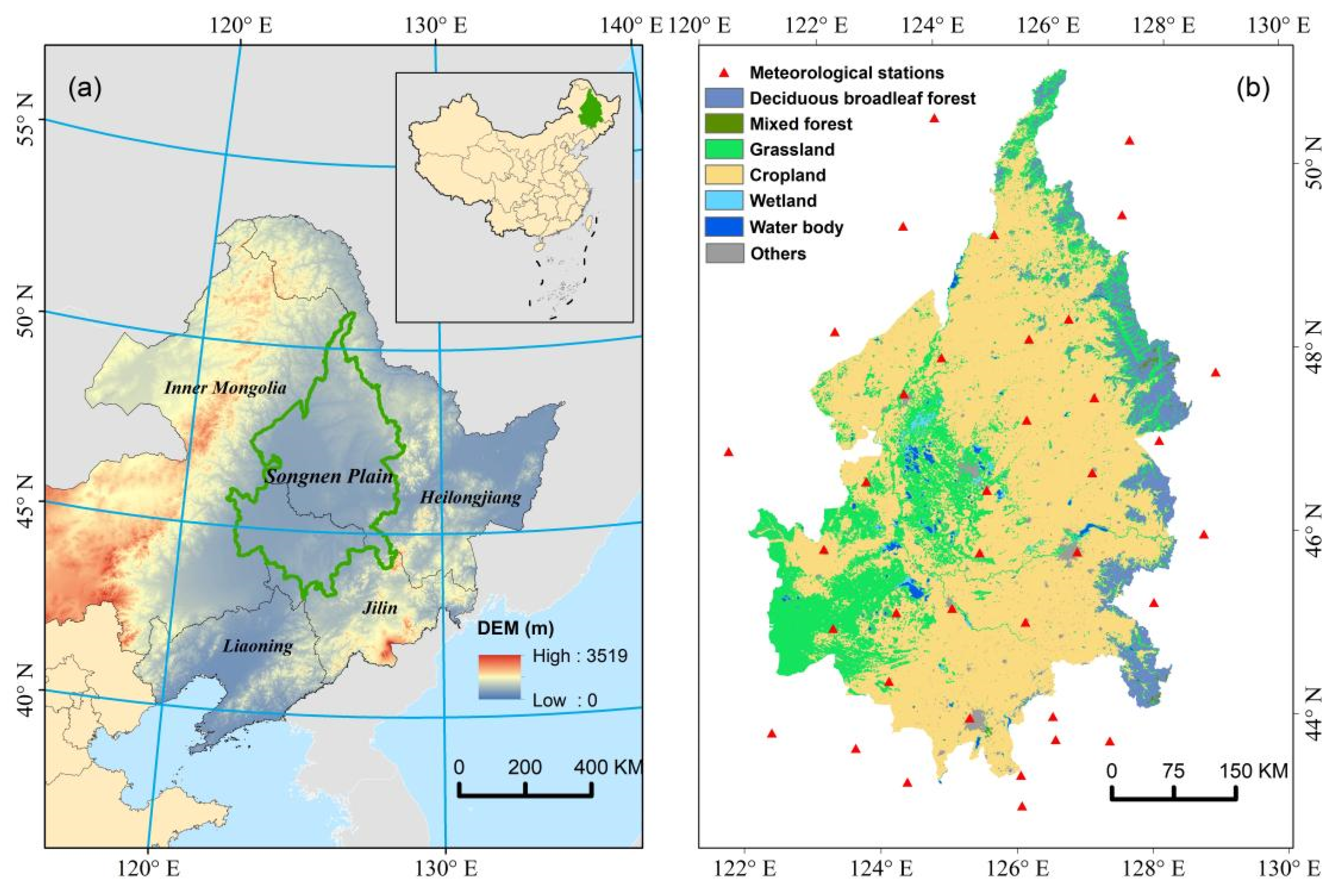
The Songnen Plain is located in northeastern China, spanning the provinces of Heilongjiang and Jilin. Together with the Three Rivers Plain and the Liaohe Plain, it constitutes the most extensive plain in China (Figure 1). It has a temperate monsoon semi-arid, semi-humid climate. The average annual precipitation is between 220 and 420 mm [30], mainly concentrated in summer (June–August), with an average temperature of 22–24 °C. The average annual evaporation ranges from 1250 to 1650 mm [29], which is almost four times of the precipitation. The region suffers from drought in different degree every year, known as “nine droughts in a decade”. It is one of the ecologically fragile agro-pastoral ecotones in northern China.
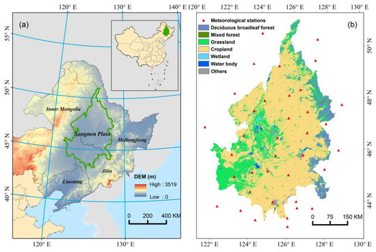
Figure 1.
(a) Location of the study area with DEM, (b) land cover type (2020).
2.2. Data and Pre-Processing
2.2.1. Climate Data
In this study, we used two climatic variables, i.e., temperature and precipitation, to calculate SPEI. Monthly data of 37 meteorological stations during 2000–2020 were obtained from the National Meteorological Information Center of China (http://data.cma.cn/ (accessed on 30 May 2021)), which were consistent with the time period of MODIS data. To maintain data consistency for subsequent calculations, both SPEI data (calculated from meteorological data) and MODIS LAI, ET, GPP data were removed seasonality in the same way. The details for the operation are given in the Section 2.3.
2.2.2. MODIS LAI Product
As an essential parameter to characterize the biophysical changes and canopy structure of vegetation, LAI directly impacts the transpiration efficiency, photosynthesis, and energy balance of vegetation [21]. We obtained the 8-day MODIS LAI product (MOD15A2) with a spatial resolution of 500 m for the 2000–2020 period from the Land Processes Distributed Active Archive Centre (LP DAAC) at https://www.earthdata.nasa.gov/eosdis/daacs/lpdaac (accessed on 2 June 2021). According to the seasonal characteristics of vegetation growth in the study area, plants enter dormancy from November to March of the following year [31,32]. Thus, we used LAI from April to October of each year. Based on the interface provided by ArcGIS 2.7 and the Python platform, the 8d LAI was synthesized into monthly data using the average method.
2.2.3. MODIS ET Product
Evapotranspiration is a key process in hydrologic cycle. The evapotranspiration data were provided by the MODIS product (MOD16A2) based on Penman-Monteith method from LP DAAC (https://www.earthdata.nasa.gov/eosdis/daacs/lpdaac (accessed on 2 June 2021)), which has an 8-day temporal interval and 500 m spatial resolution. ET reflects information on surface water and heat fluxes, which is closely related to the physical properties of the soil, the physiological activity of plants, and the formation of biological production. Due to the ability of vegetation water and carbon sequestration, surface evapotranspiration will alter accordingly when vegetation changes [21].
2.2.4. MODIS GPP Product
GPP refers to the total organic carbon fixed by organisms through photosynthesis, which is a vital variable of the global carbon cycle. It is one of the most important indicators of ecosystem function. We obtained the Terra/MODIS MOD17A2 8-day GPP data with a spatial resolution of 500 m, which are calculated by the light-use efficiency model (PSN) (https://www.earthdata.nasa.gov/eosdis/daacs/lpdaac (accessed on 2 June 2021)) [33].
2.2.5. Land Use Data
The MODIS MCD12Q1 Collection 5 (land-cover product) was used. This yearly global land cover data has a spatial resolution of 500m. We downloaded the land cover map during 2001–2020 from the MODIS official website (https://www.earthdata.nasa.gov/eosdis/daacs/lpdaac (accessed on 2 June 2021)). We adopted the classification scheme of the International Geosphere-Biosphere Programme (IGBP), including 11 natural vegetation types, three developed and mosaic land types, and three non-vegetated land types. The land cover in the Songnen Plain was summarized into seven types, including deciduous broadleaf forest, mixed forest, grassland, cropland, wetland, water body, and other types [31].
2.3. SPEI Calculation
The standardized precipitation evapotranspiration index (SPEI), proposed by Vicente-Serrano [34], can evaluate the aridity or wetness status of a region on multiple time scales. It is calculated as:
where Pi and PETi is the precipitation and the potential evapotranspiration in month i, respectively. The potential evapotranspiration is commonly estimated by the Thomthwaite and Penman-Monteith equations. The calculation is listed as follows:
where D represents cumulative water deficit, k is the time scale (month), and n is the number of calculations.
To ensure the consistency of spatial resolution, the gridded site data (500 m spatial resolution) was generated using the ordinary Kriging interpolation method within ArcGIS. The Kriging method is more advantageous for the interpolation of climatic variables [35] in areas with a uniform distribution of meteorological stations and minimal changes in elevation [36,37]. Most of the physical geographic data are non-linear. Considering the requirement of linear data in the subsequent model, we calculated the monthly anomaly of each variable (for example: the anomaly in April 2001 is the difference between value in April 2001 and multi-year average value in April) to partially eliminate the seasonality of original data.
2.4. Trends Analysis
Trend analysis methods are usually used to reveal the characteristics of variables over time. Among them, the Theil-Sen slope test is a type of regression analysis that has better robustness to missing data and outliers than the commonly used ordinary least square (OLS) regression [38,39]. As a method of determining the significance of trends [40,41], the Mann-Kendall test is often combined with the Theil-Sen slope test. It is a nonparametric statistical test that does not require the data to be restricted to a specific distribution and is less subject to outliers. We chose these two methods to conduct trend analysis and test the data.
2.5. VAR
VAR models are mainly used to predict and analyze the dynamic impact of random disturbances to the system, including the magnitude, positive and negative directions, and duration of the impact [19,20]. We used the Granger causality test and impulse response analysis methods that are suitable for exploring the relationship of geographical variables to assess the temporal dynamics and cumulative effects of drought-ecosystem function interactions in the Songnen Plain from 2000 to 2020 based on SPEI, LAI, ET, and GPP variables.
In a VAR model, each variable is a linear function of its own lagged value and the lagged values of the other variables. The general mathematical expression of the model is:
where yt denotes a vector of K variables (i.e., variables in the system that are explained by other variables, often called “dependent variables”) assigned a spherical perturbation term of the same dimension at time t and ut (i.e., a white noise process).μ is a K × 1 column vector of constant terms, A1,..., Ap is a matrix of regression coefficients of dimension K × K, and p is the lag length [19,42]. The p parameter determines how much prior information on all variables (i.e., lag time) is included in the model to predict future behavior [43].
Herein, Equation (3) is written in matrix form taking SPEI and LAI as an example:
Granger causality test is a statistical hypothesis testing method [44] that can be applied to time series data analysis. Assuming there exists variables X and Y, if the prediction effect of variable Y is better than that of Y only predicted by the past information of Y, namely, variable X helps to explain the future changes of variable Y, then variable X is considered to be the Granger cause of variable Y, and vice versa. Essentially, two regression models containing X, Y, and Y only are established, respectively. Then, the residual sum of squares of these two models is used to construct the F-statistic to determine the relationship with the original hypothesis, i.e., the existence of causality. Here, we use this method to assess whether there is a potential causal relationship between SPEI, LAI, ET, and GPP.
Note that the Granger causality test requires the input time series to be stable, whereas physical geography data generally has seasonality. Thus, it is necessary to remove seasonality from the data. Data stability is judged according to the ADF (Augmented Dickey-Fuller) coefficients. The results are scientific only when all variables involved in the modeling are cointegrated with the same order.
After making a judgment about the existence of causality between variables, impulse response analysis can help to understand the direction and strength of the relationships between the variables more deeply. The impulse response function is a causal analysis method to study the relationship between variables within a dynamic system, which has been popularized along with the development of the VAR model. The function is expressed based on the Wold moving average representation of the VAR(p) process, measuring the response process of current and future values of one variable over time after being subjected to a positive impulse of another variable [45], which is described as follows:
Additionally, the cumulative impulse response function is used to examine the cumulative effects that a change in a variable in the system at a given moment will have on the system internally over a future period. It can be obtained by iteratively summing the coefficient matrix as follows:
This matrix can be understood as the cumulative response of a variable in the system over a period of s after an impulse generated by another variable. The (i,j) coefficient of matrix ϕs is interpreted as the variable SPEIt generating an impulse at a given moment. The variable LAIt+s is the cumulative response in the period s (s = 1, 2, … n) after the impulse. We analyzed the impulse responses of SPEI with LAI, ET, and GPP in different vegetation types and the cumulative impulse responses of the study area to explore the patterns of temporal changes in SPEI and the above three ecosystem functional parameters after exerting a positive standard deviation impact on each other within 12 months and the cumulative effects.
3. Results
3.1. Change Trends of SPEI and Ecosystem Function Indicators
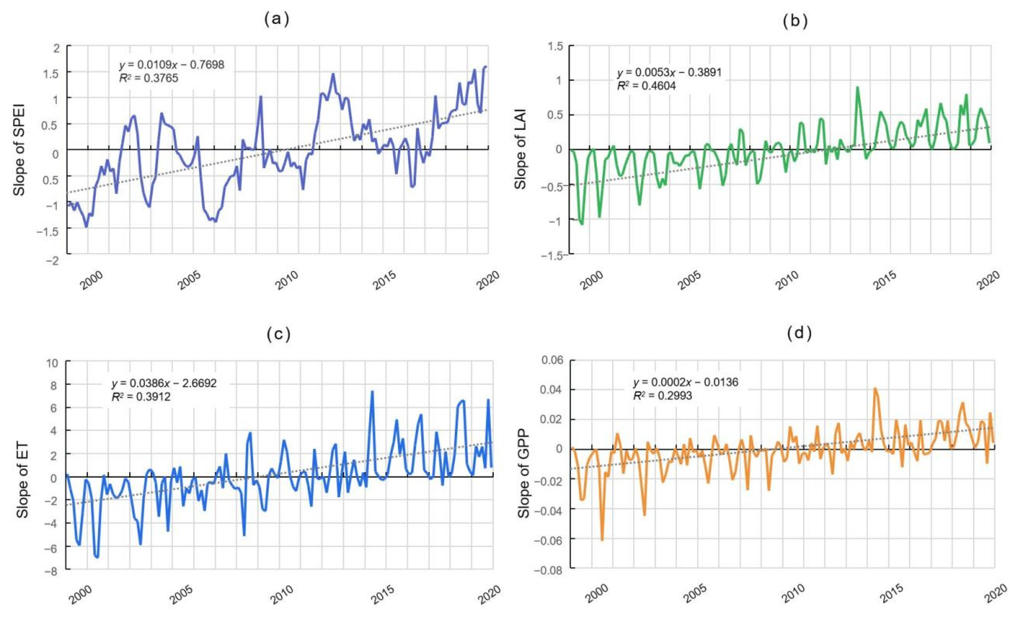
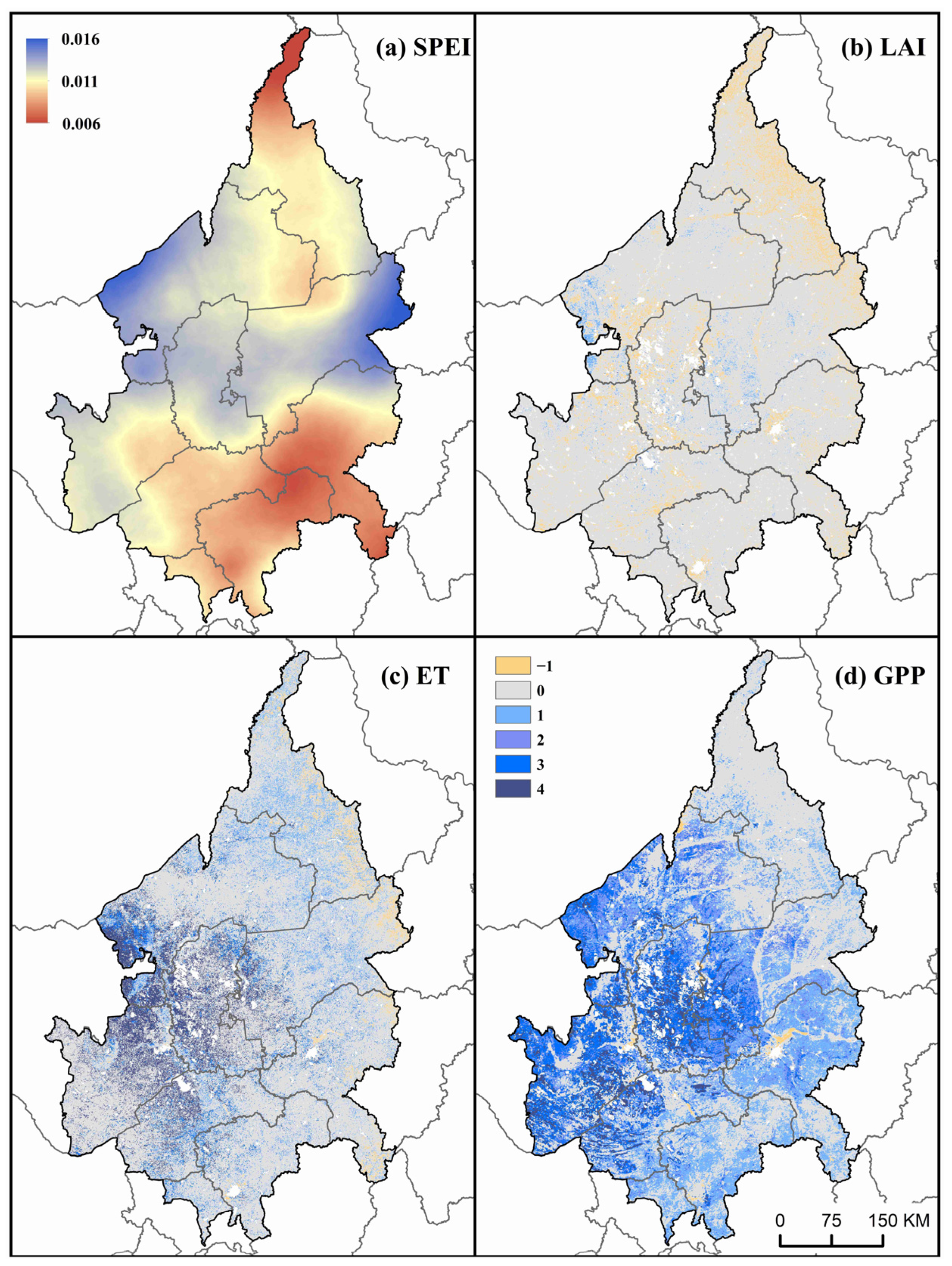
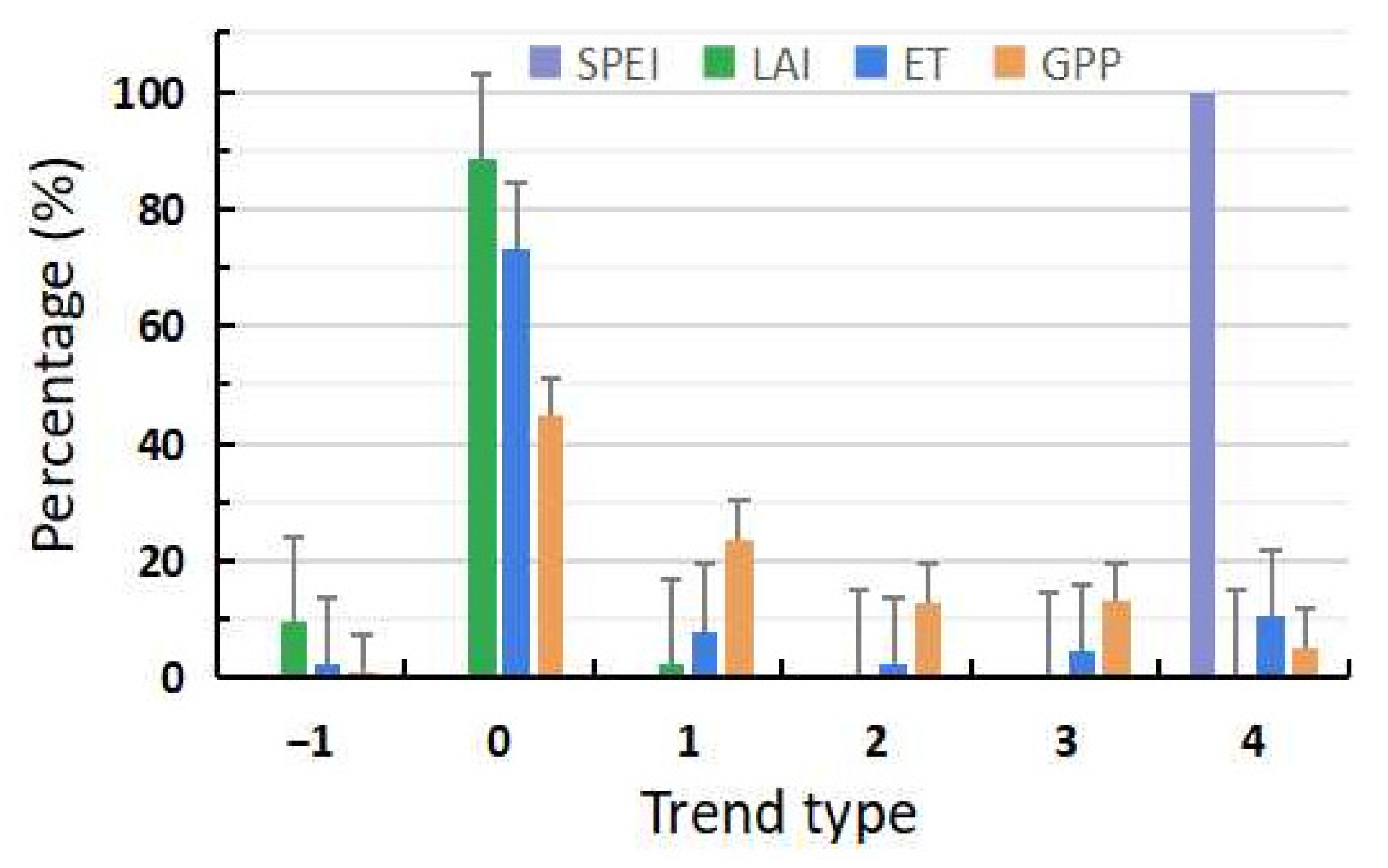
Figure 2 shows the temporal trends of the SPEI, LAI, ET, and GPP for the period of 2000–2020 using a linear regression equation. Four variables showed increasing trend, of which ET had the highest slope of 0.0386 mm/month (p < 0.05). The rest followed a descending order of SPEI > LAI > GPP. The spatial distribution of the trend derived from the Theil-Sen + MK method is illustrated in Figure 3. The trends were classified into three major types owning a total of nine characteristics (Table 1). Spatially, SPEI showed different degrees of increasing trend. Centering on the central region, the trend of SPEI decreased gradually towards the north-south direction, while it increased along the east-west direction. The most remarkable trend of increasing SPEI was found in the central grassland, wetland, and cropland. LAI tended to be unchanged, accounting for 88.34% of the total area (Figure 4). The pixels with trend value of −1 were scattered throughout the study area (taking up 9.43%) and were more concentrated in the northeastern fringe and the central areas. In the central area, the pixels of insignificantly decreasing trend were mixed with those of insignificant increasing trend. ET showed an increasing trend overall (occupying about 24.87% of the total pixels). We found that ET radiated outward from the mid-west of the study area (mainly covered by grassland), and the increasing trend decreased gradually. In the forest of the northeastern fringe, ET showed an insignificant decreasing trend, which was similar to LAI. From 2000 to 2020, the pixels with an increasing trend of GPP accounted for 54.94%. Compared with LAI and ET, the number of pixels showing no change in GPP were smallest (taking up 44.55% of the total pixels). In southwestern grassland, the pixels of significant increase and extremely significant increase in GPP (i.e., trend types 3 and 4) were clustered. In the north of the study area, GPP showed no change trend, and pixels with decreasing trend only occupied about 0.51% of the total pixels.
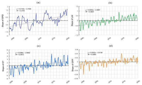
Figure 2.
Trends of SPEI (a), LAI (b), ET (c), and GPP (d) from 2000 to 2020 (p < 0.05).

Figure 3.
The spatial distribution of SPEI, LAI, ET and GPP trends from 2000 to 2020. LAI, ET and GPP are expressed using the same color table. SPEI shows significant increase trend (p < 0.05) throughout the study area, expressed in a stretched mode.

Table 1.
Change trend types of four variables.

Figure 4.
The pixel proportions of SPEI, LAI, ET, and GPP trend types from 2000 to 2020.
3.2. The Causality between SPEI and Ecosystem Function Indicators
To evaluate the relationship between ecosystem function and drought level, three groups of two-way experiments were conducted between SPEI and LAI, ET and GPP using Granger causality analysis, respectively.
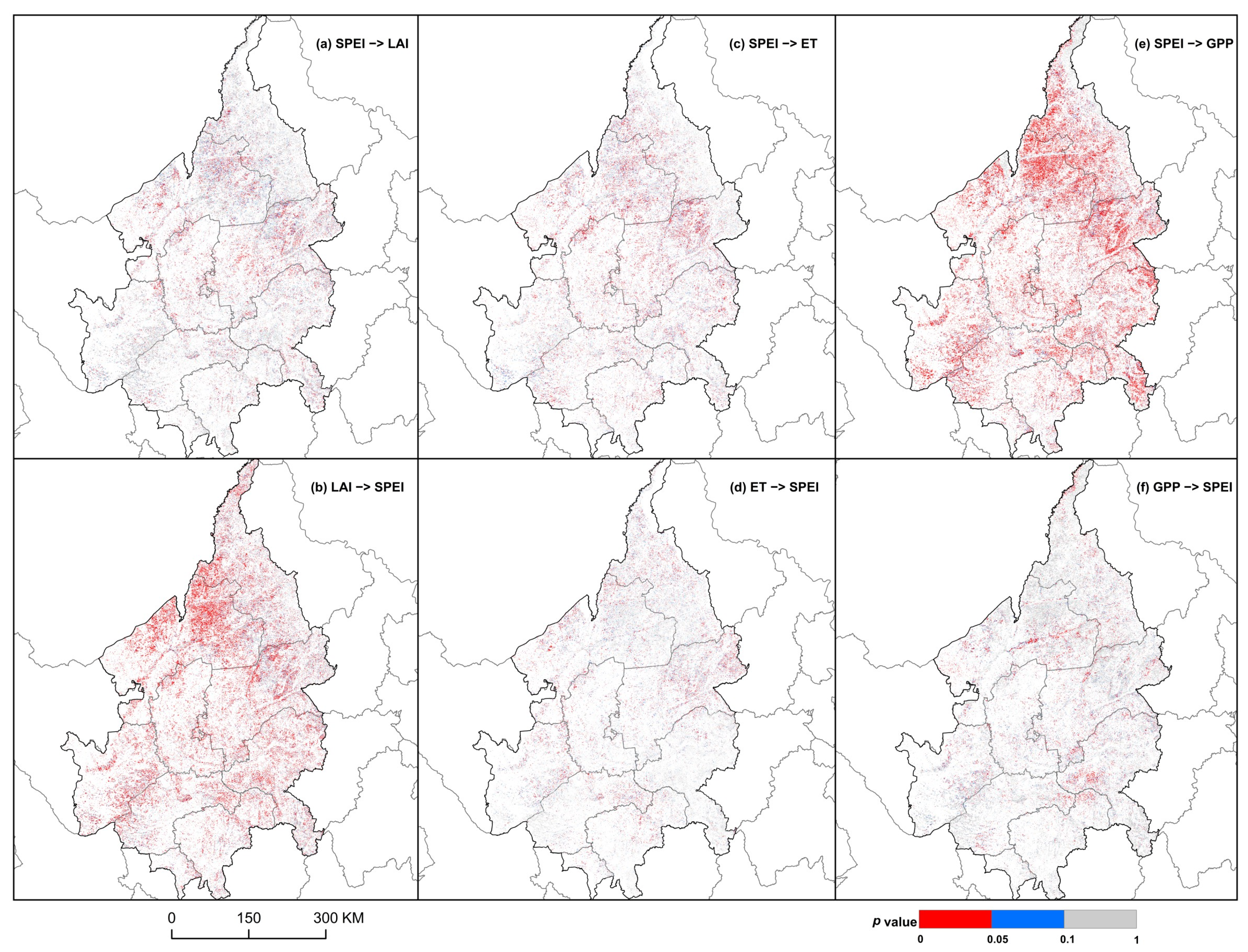
Seen from Figure 5a,b, there existed a causal relationship between SPEI and LAI in the particular area. At two significance levels of p < 0.05 and p < 0.1, the pixels with the causal relationship from LAI to SPEI took up 32.31% and 44.8% (Figure 6) of the total pixels, respectively, which are higher than that of SPEI to LAI (16.2% and 26.81%). The pixels showing SPEI-LAI causality were mainly observed in the central-northern part of the study area (Figure 5a). In contrast, LAI-SPEI causality was significant in the central-northern and eastern part of the cropland (Figure 5b). The proportions of causally significant pixels of SPEI to ET were 16.85% (p < 0.05) and 27.78% (p < 0.1), which were greater than those of ET to SPEI (10.61%, 18.79%). Overall, the number of insignificant pixels was the highest, implying that the bidirectional causality between SPEI and ET in the study area was weaker than the other two groups of variables.
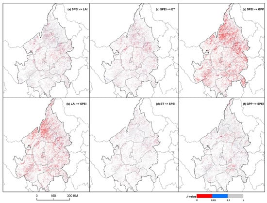
Figure 5.
The significance level (p-value) of Granger causality. (a,b) interactions between SPEI and LAI; (c,d) interactions between SPEI and ET; (e,f) interactions between SPEI and GPP. The pixels with insignificant trends are in grey color.
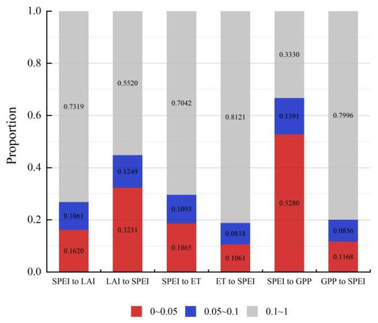
Figure 6.
The proportion of pixels at different significance levels in Granger causality of four variables.
The spatial distribution of the causality between SPEI and GPP was not consistent. Moisture condition had an impact on the photosynthesis in more areas, taking up 52.8% of the total pixels (p < 0.05), especially concentrated in the northern region (Figure 5c). Conversely, the area where vegetation photosynthesis affected moisture conditions was small with scattered pixels (Figure 5f). In the three groups of bidirectional experiments, SPEI had a greater influence on GPP, with more significant pixels. Compared with ET and GPP, the areas of SPEI response to LAI changes were larger. Spatially, the pixels that were affected by drought changes or had a regulating effect on external moisture showed highest aggregation in the northern cropland.
3.3. Interactions between SPEI and Ecosystem Function Indicators
3.3.1. SPEI and LAI
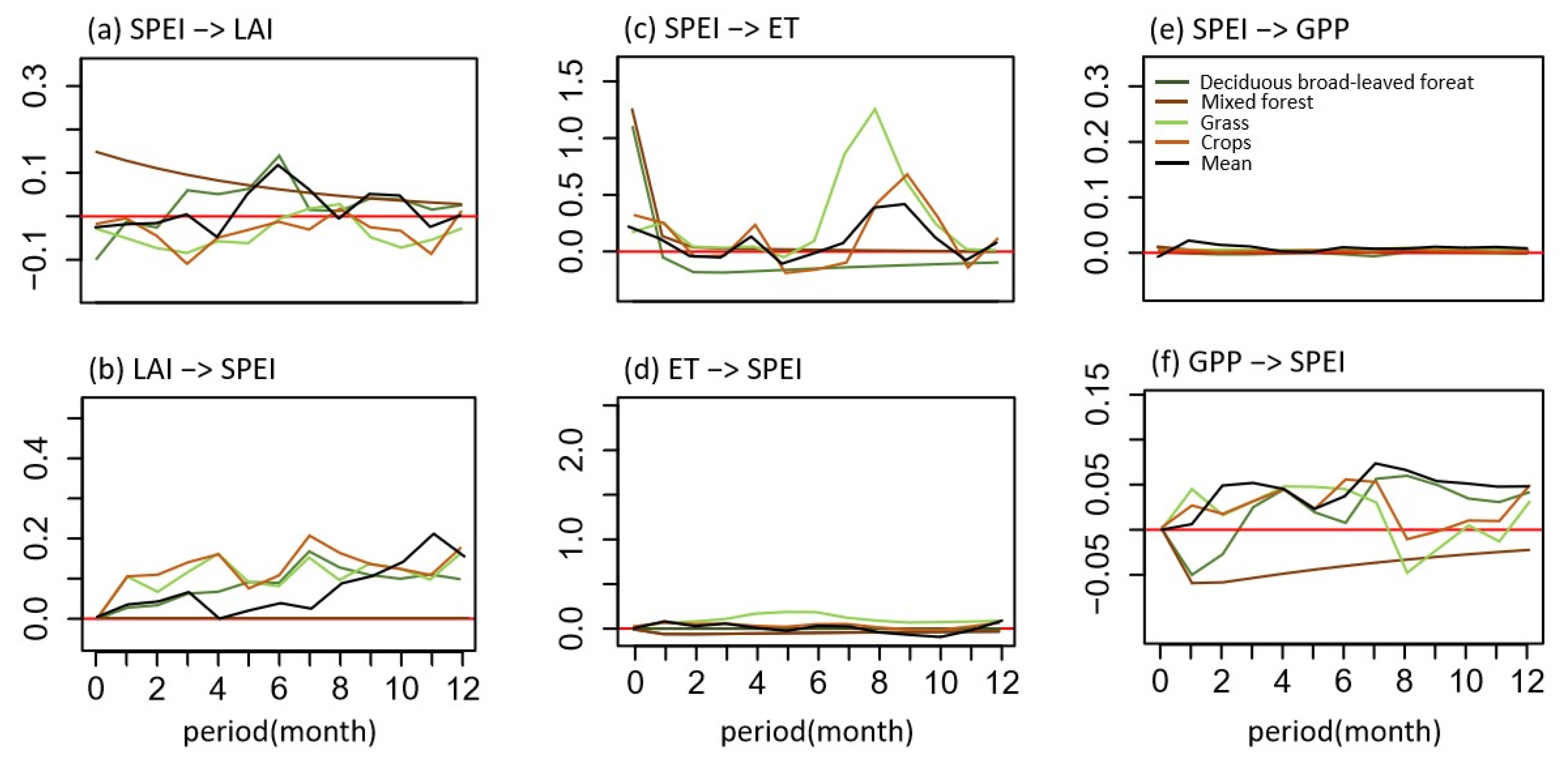
The impulse response analysis of SPEI and LAI was shown in Figure 7a, where the y-axis indicated the standard deviation of SPEI-induced LAI at a lag of n months. After an positive impact of SPEI on LAI, the response trend of deciduous broadleaf forest was similar to the mean curve. Namely, after three months of negative response, LAI started to respond positively and reached its peak in the sixth month. In terms of the cumulative effect, pixels of positive value accounted for more than 80% of the total. LAI of forestland were less affected by the changes of moisture conditions. On the contrary, the response curves of deciduous broadleaf forest, grassland, and cropland were similar in the direction of LAI to SPEI, with all positive responses within 12 months and the greatest response value in the 7th month, while the mixed forest always showed no significant change (Figure 7b). The pixels of positive cumulative impulse response coefficients occupied about 84.35% of the total (Figure 8a,b). There are more pixels of negative values (15.66%) in the direction of LAI to SPEI. We could infer that when the climate in the study area became wetter, vegetation cover would increase in most areas. Such changes in moisture condition might cause negative effects on grassland and cropland for a certain period. However, the cumulative effect was still dominated by the positive side. In contrast, the better vegetation growth would have the improved effect on regional moisture conditions, thus the drought would alleviate.
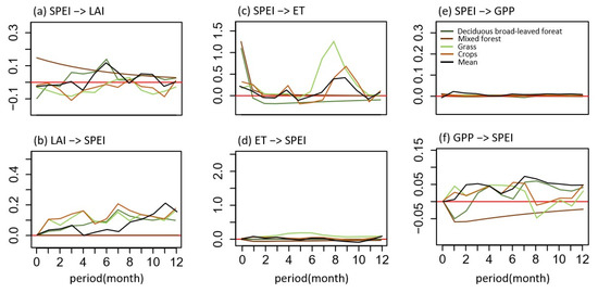
Figure 7.
Impulse responses showing the trend with time of SPEI and LAI (a,b), ET (c,d), and GPP (e,f) of different vegetation types after giving shocks to each other. The y-axis represents standard deviation (i.e., the standard deviation that a variable causing another variable at a lag of n months).
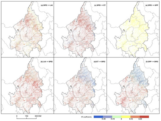
Figure 8.
The cumulative impulse coefficients in 12 months after each group of variables were impacted with each other, i.e., SPEI and LAI (a,b), ET (c,d), GPP (e,f).
3.3.2. SPEI and ET
Figure 7c illustrates the impulse response of SPEI on ET for different vegetation types. When SPEI increased, the ET of mixed forest and deciduous broadleaf forest had the maximum positive response at the beginning of the shock. The responses decreased rapidly within the following month. Subsequently, the response value of ET in mixed forests tended to be 0, while the deciduous broadleaf forest started with the negative response trend. The change trends of grassland and cropland were basically synchronized, showing positive and negative fluctuations. The maximum positive responses were observed in August and September, and thereafter the response gradually stabilized. From the cumulative effect (Figure 8c,d), impulse coefficients in about 81.41% of the pixels were greater than 0 in the Songnen Plain, whereas the negative pixels were mainly found in the forests on the northeast border. In the direction of ET to SPEI, the response of grassland was greater than 0 in all 12 months, and peaked in June. Although cropland and mixed forest had the opposite responses compared with grassland, their ET were also the most sensitive to the impact of SPEI in the first month. Deciduous broadleaf forest showed no significant change in ET (Figure 7d). From Figure 7d and Figure 8, positive accumulation in the direction of ET to SPEI dominated in the study area, but the pixels of negative response values accounted for 36.84% and were mainly found in forest land and the northern cropland. On the whole, when the regional wetness rose, evapotranspiration in most areas would increase accordingly. However, ET of forest land tended to decrease after experiencing an increasing response in the first two months. In turn, when ET increased, the northern and northeastern regions (mainly covered by forest land and cropland) had a trend toward drought, accounting for about 1/3 of the landscape, while the remaining regions were wetting.
3.3.3. SPEI and GPP
Moisture condition in the growing environment affects the carbon sequestration capacity of plants to some extent. Drought tends to reduce the gross primary productivity by inhibiting the photosynthesis [3,46,47]. However, the time-lag and cumulative effects of photosynthetic intensity changes on environmental wetness in different region need to be further analyzed. In this study, after a standard amount of SPEI shock to GPP, the photosynthesis of the main vegetation types in 12 months was positively improved under more humid conditions, but the response intensity was relatively low compared with the previous groups of experiments (Figure 7e and Figure 8e). GPP determines the initial material and energy of a terrestrial ecosystem. The response of SPEI to increasing GPP was shown in Figure 7f and Figure 8f. A negative peak of response in the mixed forest was observed in January, whereas the cumulative effect of other three vegetation types reached peaks between June and August. Nearly half of the study area had positive cumulative coefficients in the direction of GPP to SPEI, showing a similar spatial distribution to Figure 8d. The cropland and forests in the northern area tended to be dry with the increase in GPP, while grassland and cropland in other regions were getting wet, accounting for about 50.64% of the total.
4. Discussion
4.1. Spatiotemporal Variations of Drought and Ecosystem Function
In our study, we found that the drought stress in the growing season in the Songnen Plain from 2000 to 2020 tended to alleviate. The ecosystem function indicators including LAI, ET, and GPP also showed an increasing trend (Figure 2 and Figure 3). Spatially, SPEI highly significant increased across the study area. There were few changes in the area of vegetation cover, and from the analysis of land use type changes (Figures S1 and S2), we can see that almost 87% of the total area was unchanged over the past two decades. The decreasing trend in LAI was found in the central grassland and forests on the northeastern border. The main land use change processes included the conversions from grassland to cropland (8.2%) and forest to grassland (0.59%). ET and GPP showed increasing trends. Our findings are broadly consistent with previous studies [29,48,49,50]. Under a stable status of vegetation cover, wetting climate may explain the increase in ET and GPP in the Songnen Plain during past 21 years (Figure S3). Previous studies indicated that vegetation in the study area was severely degraded during 2003–2012 due to intensive human activities [30] and significant expansion of cropland [51], which were similar to our results. To curb unceasing degradation of the ecosystem and ensure sustainable regional development, the local government has implemented many ecological restoration projects. For instance, the Regulations of Grasslands in Heilongjiang was promulgated in 2006 [52], requiring that the grasslands in the Songnen Plain to be prohibited from grazing the slightly and moderately degraded grasslands outside the Songnen Plain to be implemented seasonal rest-grazing, and severely degraded, sandy, and alkaline grasslands to be carried out grazing rest. The ecosystem function in the study area had been relatively stable for the period of 2000–2020, benefiting from the effectiveness of conservation measures, whereas the conversion of grassland into cropland still occured in some areas.
4.2. Causal Relationship between Drought and Ecosystem Function
In general, only if variable a improves the accuracy of predicting b variable, a is called the Granger reason of b. In this study, there existed overall bidirectional causality between SPEI and LAI, ET, and GPP, implying a bidirectional link between ecosystem function and drought in the Songnen Plain to varying degrees, which was consistent with some previous studies [47,53]. In particular, we found that SPEI had the highest number of pixels (taking up 52.8% and 66.71%) as the Granger cause of GPP at both p < 0.05 and p < 0.1 significance levels. Wagle et al. [24,54] came to a similar conclusion that vegetation photosynthesis was more sensitive to drought than ET. This is because vegetation closes its stomata to maintain its function under drought conditions, resulting in a decrease in stomatal conductance and xylem conductance, which will directly impact photosynthesis. In terms of the regulation of ecosystem function to drought, LAI as the Granger causes of SPEI had the greatest number of pixels, accounting for 32.31% (p < 0.05) and 44.8% (p < 0.1), respectively. By constructing a two-way coupled land-air model of vegetation dynamics, Zhang et al. [55] found that the increase in vegetation coverage in the Loess Plateau led to a series of chain reactions such as the decrease in albedo, the increase in net radiation, air humidity and local water vapor flux. The land-atmosphere exchanges had positive feedback on regional precipitation and then alleviated the drought. Among three functioning indicators we selected, the increase in LAI may have played more active roles in migrating the drought in the Songnen plain during the studied period.
4.3. Lag and Cumulative Effects between Drought and Ecosystem Function
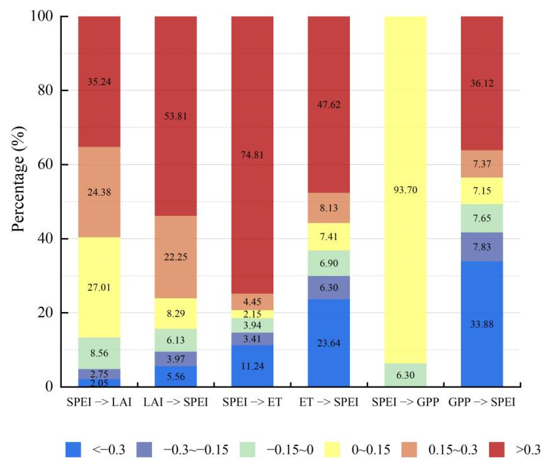
In this study, we found that the time-lag and cumulative relationships between SPEI and ecosystem function indicators varied among species and geographical distribution (Figure 8 and Figure 9). In the Songnen Plain, SPEI and LAI were both positively improved within 12 months after mutual impact, namely becoming wetter or having increased vegetation cover. The rising wetness in the study area was followed by a predominantly increasing trend in ET. By contrast, as an increase in ET increased, SPEI of more than half of the pixels increased. Meanwhile, more areas showed a trend toward drought. In the northeast areas dominated by forests, the pixels with negative impulse response coefficients were distributed concentratedly. The increased humidity will hinder the rate of water vapor movement in evapotranspiration. Woody plants with greater evapotranspiration have the potential to cause regional drought when moisture conditions are constant [56]. In the last 21 years, the Songnen Plain has become more humid, showing an increasing GPP almost in the entire study area. In the opposite direction, the increase in GPP was followed by a drought trend in about half of the total area, mainly in the northeast and in forests along the southwest border. Generally, the composition, structure, and function of forests are closely related to water. Forests have essential adaptive effects and feedback on water factors at various scales [46]. In some areas, the problem of excessive water consumption in forests affects regional water movement and cycle [57].
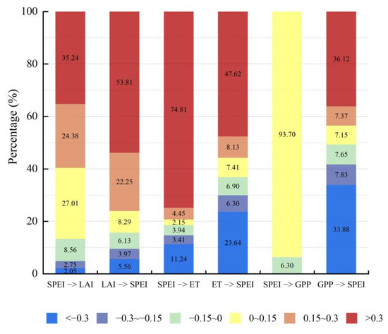
Figure 9.
The proportion of pixels of cumulative pulse coefficient among SPEI and ecosystem functional indicators.
Our experiments showed that there existed a certain lag between moisture conditions and vegetation in the Songnen Plain. The greatest response were in 6–8th months later, and the mutual impact tended to disappear after one year. Some studies indicated that the most sensitive period between vegetation and moisture in arid and semi-arid regions was from April to July [58,59]. Compared with woody plants, herbaceous plants were more sensitive to external conditions. Due to their shallow root systems and lower xylem hydraulic resistance, grasslands prone to the drought stress [11,12]. The relationship between ecosystem function and moisture conditions in the area dominated by the same vegetation type varied depending on the geographical location, which might be related to spatial differences in climate [25]. In summary, GPP was most affected by water conditions in the Songnen Plain, followed by vegetation cover (LAI) with the second broadest coverage; ET is the smallest but similar to LAI. As a previous study indicated, the correlation between LAI and biomass-related variables was high in semi-arid regions globally [27].
4.4. Limitations and Future Directions
The accuracy of SPEI generated by the interpolation of site-based precipitation and temperature data might have some limitations. SPEI was calculated based on precipitation and potential evapotranspiration in this study. Many studies have reported that the increase in potential evapotranspiration will exacerbate the aridity of a regional environment [60]. Therefore, how the complex interactions between different environmental factors affect vegetation growth need to be further examined. In addition, the construction of the VAR model requires the data to pass the stability test, which will result in partial data loss. Due to the difficulties of this model for large-scale data analysis [61], we synthesized 8-day MODIS data into monthly-scale time series data. In a future study, other data processing methods such as Toda and Yamamoto procedure [62] can be tried to improve the efficiency of data utilization and analysis so as to meet the requirement of quantitatively revealing the relationship between drought and ecosystem function response at fine scale.
5. Conclusions
In this study, we investigated the trends of drought extent (SPEI), vegetation cover (LAI), evapotranspiration (ET), and photosynthesis (GPP) in the Songnen Plain of northeastern China from 2000 to 2020 at the pixel scale. The bidirectional causality, time-lag, and cumulative response among the factors were analyzed to reveal the interactive relationship between drought and ecosystem function. In the last 21 years, the drought situation in the Songnen Plain had improved in different degrees. Vegetation cover changed insignificantly, whereas both ET and GPP showed increasing trends. Some degradation were found in the forest land. There was a certain degree of bidirectional causality between SPEI and LAI, ET, and GPP, among them the number of pixels were highest in the responding relationship of LAI-SPEI and SPEI-GPP. The response time and intensity of the variables to the shocks varied significantly among species. The greatest response intensity were basically concentrated between 6th and 8th months, roughly having a positive mutual contribution. The cumulative impulse response coefficients showed significant spatial differences and positive value of pixels took predominantly, indicating that LAI, ET, and GPP in most areas increased in 12 months after the impact as the Songnen Plain became wetting. On the other hand, the increase in values of ecosystem function indicators would promote the study area toward a wetter direction. The negative response areas were mainly distributed in the northeast (edge of the Xiaoxing’an Mountains) and southeast border areas, dominated by woody plants. The above results indicate that there existed some time-lag and cumulative effect between water conditions and plant interactions in temperate semi-arid and semi-humid transition areas, and they were varied among regions and vegetation species.
Supplementary Materials
The following supporting information can be downloaded at: https://www.mdpi.com/article/10.3390/rs14225887/s1. Figure S1. Area changes of major land use/cover during 2001–2020. Figure S2. Spatial distribution and the area percentage of major land use type change types over three different periods in the Songnen Plain. Figure S3. Change trends of: (a) Temperature, (b) Precipitation from 2000 to 2020. Figure S4. Spatial distribution of: (a) Temperature, (b) Precipitation from 2000 to 2020 (p < 0.05).
Author Contributions
H.L.: Conceptualization, Methodology, Investigation, Writing–original draft, Visualization. F.H.: Conceptualization, Resources, Writing—review & editing, Supervision, Funding acquisition. X.H.: Methodology, Writing—review & editing. P.W.: Data processing, Writing—review & editing. All authors have read and agreed to the published version of the manuscript.
Funding
This work was supported by the Natural Science Foundation of Jilin Province, China (Grant No. 20220101155JC), the National Natural Science Foundation of China (Grant No. 41571405), and the Education Department of Jilin Province, China (Grant No. JJKH20211289KJ).
Data Availability Statement
Not applicable.
Acknowledgments
The authors would like to thank the reviewers and editors for their valuable comments and suggestions.
Conflicts of Interest
The authors declare no conflict of interest.
References
- Li, Y.; Xie, Z.; Qin, Y.; Xia, H.; Zheng, Z.; Zhang, L.; Pan, Z.; Liu, Z. Drought Under Global Warming and Climate Change: An Empirical Study of the Loess Plateau. Sustainability 2019, 11, 1281. [Google Scholar] [CrossRef]
- Wang, Z.; Zhong, R.; Lai, C.; Zeng, Z.; Lian, Y.; Bai, X. Climate change enhances the severity and variability of drought in the Pearl River Basin in South China in the 21st century. Agric. For. Meteorol. 2018, 249, 149–162. [Google Scholar] [CrossRef]
- Zhao, M.; Running, S.W. Drought-induced reduction in global terrestrial net primary production from 2000 through 2009. Science 2010, 329, 940–943. [Google Scholar] [CrossRef] [PubMed]
- Zhao, M.; Running, S.W. Response to Comments on “Drought-Induced Reduction in Global Terrestrial Net Primary Production from 2000 Through 2009”. Science 2011, 333, 1093. [Google Scholar] [CrossRef]
- Mcdowell, N.G. Mechanisms Linking Drought, Hydraulics, Carbon Metabolism, and Vegetation Mortality. Plant Physiol. 2011, 155, 1051–1059. [Google Scholar] [CrossRef]
- Zhao, A.; Zhang, A.; Cao, S.; Liu, X.; Liu, J.; Cheng, D. Responses of vegetation productivity to multi-scale drought in Loess Plateau, China. Catena 2018, 163, 165–171. [Google Scholar] [CrossRef]
- Chu, H.; Venevsky, S.; Chao, W.; Wang, M. NDVI-based vegetation dynamics and its response to climate changes at Amur-Heilongjiang River Basin from 1982 to 2015. Sci. Total Environ. 2018, 650, 2051–2062. [Google Scholar] [CrossRef] [PubMed]
- Cooley, S.S.; Williams, C.; Fisher, J.B.; Halverson, G.H.; Perret, J.; Lee, C.M. Assessing regional drought impacts on vegetation and evapotranspiration: A case study in Guanacaste, Costa Rica. Ecol. Appl. 2019, 29, e01834. [Google Scholar] [CrossRef]
- Wen, Y.Y.; Liu, X.P.; Xin, Q.C.; Wu, J.; Xu, X.C.; Pei, F.S.; Li, X.; Du, G.M.; Cai, Y.L.; Lin, K.; et al. Cumulative Effects of Climatic Factors on Terrestrial Vegetation Growth. J. Geophys. Res. Biogeosci. 2019, 124, 789–806. [Google Scholar] [CrossRef]
- Wu, D.H.; Zhao, X.; Liang, S.L.; Zhou, T.; Huang, K.C.; Tang, B.J.; Zhao, W.Q. Time-lag effects of global vegetation responses to climate change. Glob. Chang. Biol. 2015, 21, 3520–3531. [Google Scholar] [CrossRef]
- Craine, J.M.; Ocheltree, T.W.; Nippert, J.B.; Towne, E.G.; Skibbe, A.M.; Kembel, S.W.; Fargione, J.E. Global diversity of drought tolerance and grassland climate-change resilience. Nat. Clim. Chang. 2013, 3, 63–67. [Google Scholar] [CrossRef]
- Knapp, A.K.; Carroll, C.J.W.; Denton, E.M.; La Pierre, K.J.; Collins, S.L.; Smith, M.D. Differential sensitivity to regional-scale drought in six central US grasslands. Oecologia 2015, 177, 949–957. [Google Scholar] [CrossRef] [PubMed]
- D’Orangeville, L.C.; Maxwell, J.; Kneeshaw, D.; Pederson, N.; Duchesne, L.; Logan, T.; Houle, D.; Arseneault, D.; Beier, C.M.; Bishop, D.A. Drought timing and local climate determine the sensitivity of eastern temperate forests to drought. Glob. Chang. Biol. 2018, 24, 2339–2351. [Google Scholar] [CrossRef] [PubMed]
- Peng, J.; Wu, C.; Zhang, X.; Wang, X.; Gonsamo, A. Satellite detection of cumulative and lagged effects of drought on autumn leaf senescence over the Northern Hemisphere. Glob. Chang. Biol. 2019, 25, 2174–2188. [Google Scholar] [CrossRef] [PubMed]
- Vicente-Serrano, S.M.; Gouveia, C.; Julio Camarero, J.; Begueria, S.; Trigo, R.; Lopez-Moreno, J.I.; Azorin-Molina, C.; Pasho, E.; Lorenzo-Lacruz, J.; Revuelto, J.; et al. Response of vegetation to drought time-scales across global land biomes. Proc. Natl. Acad. Sci. USA 2013, 110, 52–57. [Google Scholar] [CrossRef]
- Hoover, D.L.; Rogers, B.M. Not all droughts are created equal: The impacts of interannual drought pattern and magnitude on grassland carbon cycling. Glob. Chang. Biol. 2016, 22, 1809–1820. [Google Scholar] [CrossRef]
- Ivits, E.; Horion, S.; Erhard, M.; Fensholt, R. Assessing European ecosystem stability to drought in the vegetation growing season. Glob. Ecol. Biogeogr. 2016, 25, 1131–1143. [Google Scholar] [CrossRef]
- Wu, X.; Liu, H.; Li, X.; Ciais, P.; Babst, F.; Guo, W.; Zhang, C.; Magliulo, V.; Pavelka, M.; Liu, S.; et al. Differentiating drought legacy effects on vegetation growth over the temperate Northern Hemisphere. Glob. Chang. Biol. 2018, 24, 504–516. [Google Scholar] [CrossRef]
- Sims, C.A. Macroeconomics and Reality. Econometrica 1980, 48, 1–48. [Google Scholar] [CrossRef]
- Zheng, Y. Theory of Impulse Response Function with Applications in Macroeconomic System. Ph.D. Thesis, Nankai University, Tianjin, China, 2010. [Google Scholar]
- Mariano, D.A.; Santos, C.; Wardlow, B.D.; Anderson, M.C.; Schiltmeyer, A.V.; Tadesse, T.; Svoboda, M. Use of remote sensing indicators to assess effects of drought and human-induced land degradation on ecosystem health in Northeastern Brazil. Remote Sens. Environ. 2018, 213, 129–143. [Google Scholar] [CrossRef]
- Gouveia, C.M.; Trigo, R.M.; Begueria, S.; Vicente-Serrano, S.M. Drought impacts on vegetation activity in the Mediterranean region: An assessment using remote sensing data and multi-scale drought indicators. Glob. Planet. Chang. 2016, 151, 15–27. [Google Scholar] [CrossRef]
- Zhilong, Z.; Yili, Z.; Linshan, L.; Zengzeng, H.; Yangyang, X. The impact of drought on vegetation conditions within the Damqu River Basin, Yangtze River Source Region, China. PLoS ONE 2018, 13, e0202966. [Google Scholar]
- Wagle, P.; Kakani, V.G. Growing season variability in evapotranspiration, ecosystem water use efficiency, and energy partitioning in switchgrass. Ecohydrology 2014, 7, 64–72. [Google Scholar] [CrossRef]
- Xu, H.-J.; Wang, X.-P.; Zhao, C.-Y.; Yang, X.-M. Diverse responses of vegetation growth to meteorological drought across climate zones and land biomes in northern China from 1981 to 2014. Agric. For. Meteorol. 2018, 262, 1–13. [Google Scholar] [CrossRef]
- Zhang, Q.; Kong, D.; Singh, V.P.; Shi, P. Response of vegetation to different time-scales drought across China: Spatiotemporal patterns, causes and implications. Glob. Planet. Chang. 2017, 152, 1–11. [Google Scholar] [CrossRef]
- Li, Z.; Chen, Y.; Wang, Y.; Fang, G. Dynamic changes in terrestrial net primary production and their effects on evapotranspiration. Hydrol. Earth Syst. Sci. 2016, 20, 2169–2178. [Google Scholar] [CrossRef]
- Qu, G.; Guo, J. The relationship between different plant communities and soil characteristics in Songnen grassland. Acta Prataculturae Sin. 2003, 12, 18–22. [Google Scholar]
- Wu, X.; Na, X.; Zang, S. Application of temperature vegetation dryness index in the estimation of soil moisture of the Songnen Plain. Acta Ecol. Sin. 2019, 39, 4432–4441. [Google Scholar]
- Wang, Y.; Huang, F. Identification and analysis of ecosystem functional types in the west of Songnen Plain, China, based on moderate resolution imaging spectroradiometer data. J. Appl. Remote Sens. 2015, 9, 096096. [Google Scholar] [CrossRef]
- Li, B.; Huang, F.; Qin, L.; Qi, H.; Sun, N. Spatio-Temporal Variations of Carbon Use Efficiency in Natural Terrestrial Ecosystems and the Relationship with Climatic Factors in the Songnen Plain, China. Remote Sens. 2019, 11, 2513. [Google Scholar] [CrossRef]
- Huang, F.; Wang, P.; Chang, S.; Li, B. Rain use efficiency changes and its effects on land surface phenology in the Songnen Plain, Northeast China. In Proceedings of the Remote Sensing for Agriculture, Ecosystems, and Hydrology XX, Berlin, Germany, 10–13 September 2018; pp. 90–98. [Google Scholar]
- Zhao, M.; Heinsch, F.A.; Nemani, R.R.; Running, S.W. Improvements of the MODIS terrestrial gross and net primary production global data set. Remote Sens. Environ. 2005, 95, 164–176. [Google Scholar] [CrossRef]
- Vicente-Serrano, S.M.; Begueria, S.; Lopez-Moreno, J.I. A Multiscalar Drought Index Sensitive to Global Warming: The Standardized Precipitation Evapotranspiration Index. J. Clim. 2010, 23, 1696–1718. [Google Scholar] [CrossRef]
- Alsamamra, H.; Ruiz-Arias, J.A.; Pozo-Vázquez, D.; Tovar-Pescador, J. A comparative study of ordinary and residual kriging techniques for mapping global solar radiation over southern Spain. Agric. For. Meteorol. 2009, 149, 1343–1357. [Google Scholar] [CrossRef]
- Bao, G.; Qin, Z.; Bao, Y.; Zhou, Y.; Li, W.; Sanjjav, A. NDVI-based long-term vegetation dynamics and its response to climatic change in the Mongolian Plateau. Remote Sens. 2014, 6, 8337–8358. [Google Scholar] [CrossRef]
- Bao, G.; Jin, H.; Tong, S.; Chen, J.; Du, L. Autumn Phenology and Its Covariation with Climate, Spring Phenology and Annual Peak Growth on the Mongolian Plateau. Agric. For. Meteorol. 2021, 298, 108312. [Google Scholar] [CrossRef]
- Sen, P.K. Estimates of the Regression Coefficient Based on Kendall’s Tau. Publ. Am. Stat. Assoc. 1968, 63, 1379–1389. [Google Scholar] [CrossRef]
- Theil, H. A Rank-Invariant Method of Linear and Polynomial Regression Analysis. Nederl. Akad. Wetensch. Proc. 1992, 12, 345–381. [Google Scholar]
- Kendall, M.G. Rank Correlation Methods. Br. J. Psychol. 1990, 25, 86–91. [Google Scholar] [CrossRef]
- Mann, H.B. Nonparametric test against trend. Econometrica 1945, 13, 245–259. [Google Scholar] [CrossRef]
- Pfaff, B. VAR, SVAR and SVEC Models: Implementation Within R Package vars. J. Stat. Softw. 2008, 27, 1–32. [Google Scholar] [CrossRef]
- Wang, W.; Anderson, B.T.; Phillips, N.; Kaufmann, R.K. Feedbacks of Vegetation on Summertime Climate Variability over the North American Grasslands. Part I: Statistical Analysis. Earth Interact. 2006, 10, 1–27. [Google Scholar] [CrossRef]
- Granger, C.W.J. Investigating Causal Relations by Econometric Models and Cross-Spectral Methods. Econometrica 1969, 37, 424–438. [Google Scholar] [CrossRef]
- Lütkepohl, H. New Introduction to Multiple Time Series Analysis; Springer Science & Business Media: Berlin/Heidelberg, Germany, 2005. [Google Scholar]
- Li, H. Modern Plant Physiology, Fourth Edition. Life World 2019, 165, 293. [Google Scholar]
- Hua, T.; Wang, X.; Zhang, C.; Lang, L.; Li, H. Responses of vegetation activity to drought in Northern China. Land Degrad. Dev. 2017, 28, 1913–1921. [Google Scholar] [CrossRef]
- Zeng, L.H.; Song, K.S.; Zhang, B.; Li, L.; Wang, Z.M. Evapotranspiration estimation using moderate resolution imaging spectroradiometer products through a surface energy balance algorithm for land model in Songnen Plain, China. J. Appl. Remote Sens. 2011, 5, 053535. [Google Scholar] [CrossRef]
- Wang, Q.; Zhao, W.; Zhang, Y. Study on Ecological Environment Change of Songnen Plain Based on FVC Index. Geomat. Spat. Inf. Technol. 2021, 44, 164–167. [Google Scholar]
- Wang, Y.J.; Shen, X.J.; Jiang, M.; Lu, X.G. Vegetation Change and Its Response to Climate Change between 2000 and 2016 in Marshes of the Songnen Plain, Northeast China. Sustainability 2020, 12, 3569. [Google Scholar] [CrossRef]
- Chu, X.-L.; Zhong, L.; Dan, W.; Lei, G.-P. Effects of land use/cover change (LUCC) on the spatiotemporal variability of precipitation and temperature in the Songnen Plain, China. J. Integr. Agric. 2022, 21, 235–248. [Google Scholar] [CrossRef]
- Zhang, R.; Zhang, Y.; Pan, D.; Shen, Z.; Li, D.; Wang, J. Strategies of Grassland Ecosystem Protection and Construction in Heilongjiang Province. Heilongjiang Agric. Sci. 2008, 5, 119–121. [Google Scholar]
- Yuan, W.; Liu, D.; Dong, W.; Liu, S.; Zhou, G.; Yu, G.; Zhao, T.; Feng, J.; Ma, Z.; Chen, J.; et al. Multiyear precipitation reduction strongly decreases carbon uptake over northern China. J. Geophys. Res. Biogeosci. 2014, 119, 881–896. [Google Scholar] [CrossRef]
- Wagle, P.; Xiao, X.; Torn, M.S.; Cook, D.R.; Matamala, R.; Fischer, M.L.; Jin, C.; Dong, J.; Biradar, C. Sensitivity of vegetation indices and gross primary production of tallgrass prairie to severe drought. Remote Sens. Environ. 2014, 152, 1–14. [Google Scholar] [CrossRef]
- Zhang, B.; Tian, L.; Zhao, X.; Wu, P. Feedbacks between vegetation restoration and local precipitation over the loess plateau in China. Sci. China Earth Sci. 2021, 51, 1080–1091. [Google Scholar] [CrossRef]
- Zeng, L.; Song, K.; Zhang, B.; Wang, Z.; Du, J. Analysis of Spatiotemporal Variations in Evapotranspiration and Its Influencing Factors over the Songnen Plain in the Growing Season during the Period 2000–2008. Resourses Sci. 2010, 32, 2305–2315. [Google Scholar]
- Wang, Y. Characteristics of Photosynthesis and Water Use of Dominant Tree Species in Typical Forests and Related Factors in the Semiarid Region of Loess Plateau, China. Ph.D. Thesis, Chinese Academy of Sciences, Beijing, China, 2010. [Google Scholar]
- Liu, L.; Zhang, Y.; Wu, S.; Li, S.; Qin, D. Water memory effects and their impacts on global vegetation productivity and resilience. Sci. Rep. 2018, 8, 2962. [Google Scholar] [CrossRef] [PubMed]
- Lotsch, A.; Friedl, M.A.; Anderson, B.T.; Tucker, C.J. Coupled vegetation-precipitation variability observed from satellite and climate records. Geophys. Res. Lett. 2003, 30, 1774. [Google Scholar] [CrossRef]
- Cook, B.I.; Smerdon, J.E.; Seager, R.; Coats, S. Global warming and 21st century drying. Clim. Dyn. 2014, 43, 2607–2627. [Google Scholar] [CrossRef]
- Hyndman, R.J.; Athanasopoulos, G. Forecasting: Principles and Practice; OTexts: Melbourne, Australia, 2018. [Google Scholar]
- Toda, H.Y.; Yamamoto, T. Statistical inference in vector autoregressions with possibly integrated processes. J. Econom. 1995, 66, 225–250. [Google Scholar] [CrossRef]
Publisher’s Note: MDPI stays neutral with regard to jurisdictional claims in published maps and institutional affiliations. |
© 2022 by the authors. Licensee MDPI, Basel, Switzerland. This article is an open access article distributed under the terms and conditions of the Creative Commons Attribution (CC BY) license (https://creativecommons.org/licenses/by/4.0/).

