

Vine Canopy Reconstruction and Assessment with Terrestrial Lidar and Aerial Imaging
1
Faculty of Mechanical Engineering, University of Ljubljana, Aškerčeva 6, 1000 Ljubljana, Slovenia
2
Faculty of Agriculture and Life Sciences, University of Maribor, Pivola 10, 2311 Hoče, Slovenia
*
Author to whom correspondence should be addressed.
Remote Sens. 2022, 14(22), 5894; https://doi.org/10.3390/rs14225894
Submission received: 12 September 2022
/
Revised: 12 November 2022
/
Accepted: 15 November 2022
/
Published: 21 November 2022
(This article belongs to the Special Issue 3D Modelling and Mapping for Precision Agriculture)
Abstract
:For successful dosing of plant protection products, the characteristics of the vine canopies should be known, based on which the spray amount should be dosed. In the field experiment, we compared two optical experimental methods, terrestrial lidar and aerial photogrammetry, with manual defoliation of some selected vines. Like those of other authors, our results show that both terrestrial lidar and aerial photogrammetry were able to represent the canopy well with correlation coefficients around 0.9 between the measured variables and the number of leaves. We found that in the case of aerial photogrammetry, significantly more points were found in the point cloud, but this depended on the choice of the ground sampling distance. Our results show that in the case of aerial UAS photogrammetry, subdividing the vine canopy segments to 5 × 5 cm gives the best representation of the volume of vine canopies.
1. Introduction
In viticulture, chemical spraying remains the primary method of crop protection, despite its well-documented harmful effects on the environment, farmers, and food. Plant protection products (PPPs) should ideally be applied in the minimum amount necessary to reduce drift while providing reliable protection against pests and diseases. Societal pressure to eliminate or reduce the use of chemical sprays is increasing, leading to changes in national spraying regulations. To achieve the goal of sustainable protection and to produce a high quality and quantity of grapes, a mix of complementary approaches is needed. These include the use of more resistant varieties, spraying with biological PPPs, improving the application methodology, incorporating novel dosing algorithms and spraying techniques tailored to individual plants, and other methods and practices [1,2]. A review of measurement and spraying methods in permanent crops can be found in [3].
In recent decades, many authors have pointed out the importance of actual measurements of the parameters of the canopy being sprayed. A review of measurement and spraying methods in permanent crops can be found in [3]. Measurement of canopies and adjustment of the spray dose for permanent crops was attempted decades ago, both in vineyards and orchards. Early approaches included using the leaf wall area (LWA) [4] and tree row volume (TRV) [5], which averaged geometric canopy parameters such as thickness and height with inter-row spacing. Although this was a valuable improvement over using a constant dosage per hectare, LWA or TRV also have disadvantages. These are limited measurement accuracy due to manual estimation of orchard parameters at a limited number of points and the inability to account for general varieties of vineyard conditions, training systems and management strategies, individual plant growth, changes due to soil variations, changes in vineyard location and slope, etc.
The disadvantages of LWA and TRV methods can be overcome by the introduction of automatic measurement techniques. In the recent past, ultrasound, lidar (light detection and ranging), terrestrial imaging, and aerial imaging have been among the most commonly used sensing methods [2,3,6]. Ultrasonic methods have been in the past decade displaced [7,8,9] by optical methods due to their higher reliability, repeatability, and much better spatial resolution.
Non-destructive optical methods, including point infrared sensors, terrestrial and airborne lidar, and terrestrial and airborne imaging, offer the advantage of providing sufficient information about canopy geometric properties such as height, width, density, and so on. In the past, optical methods were limited to single-point light-sensitive infrared sensors for spray control (on/off). Optical measurement systems based on scanning infrared laser beams reflected from the object back to the sensor receiver (lidar) have only recently been introduced. The lidar measurement method is based on the principle of time-of-flight measurement from the sensor to the object and back. Some lidar sensors make additional use of frequency modulated light measurement; 2D lidars perform measurements by scanning the entire measurement plane. This is usually achieved by rotating a mirror to scan a 2D plane perpendicular to the mirror’s axis of rotation. When driving along the vineyard or orchard, the high operating frequency of up to 400 Hz per scan plane enables 3D reconstruction with a large number of points within the cloud. Terrestrial lidar allows for the collection and subsequent interpretation of plant-level data for analysis of individual plants or at the level of the entire orchard, with individual plant data averaged or otherwise processed. The data allow comparison with LWA and TWA methods [10], and the high point cloud density allows estimation [11,12,13] of distributions of tree canopy properties (including size, geometry, height, volume, cross-section, density, etc.). Measurements of tree canopy properties with lidar have a measurement uncertainty of more than 10% for leaf area [14], due to the large irregularity and 3D spatial structure with overlapping leaves and branches protruding from the tree canopy, etc. There are some other problems, including estimation of the thickness of the row when measured by methods that can only measure from one side (also applies to other terrestrial methods), the occlusion of the interior of the tree canopy by branches and leaves near the sensor, the tilt of the system and sensor, etc. In addition, it is impossible to distinguish individual branches because they may overlap considerably. Lidar has been very recently successfully used in aerial application also. In orchards, [15] succeeded with a very high reliability of 99% in detecting a number of trees and estimating canopy characteristics (TRV, LWA, canopy volume, and canopy cover) with lidar mounted on an unmanned aerial system.
Compared to terrestrial and airborne use of lidar, much fewer authors have used aerial photogrammetry in vineyards or orchards [16,17,18,19,20]. Among them, [21] measured orchard and vineyard properties using different flight heights, ground sampling distances, and sensor inclinations, achieving about R2 = 80% agreement with conventional TRV and LWA methods. The authors have found that ground sampling distance is the most important parameter in photogrammetric image acquisition. The authors frequently use multispectral cameras to measure canopy characteristics [22], and the multispectral camera acquisition approach has become one of the most widely used remote sensing methods in aerial applications.
Flight planning has emerged as an important parameter in photogrammetry applications [21,23,24]. The most important parameters of photogrammetry flight planning to achieve the desired photogrammetry result are the ground sample distance, the area of interest, the characteristics and calibration of the camera and optics, and the selection and distribution of ground control points [25] with their precise location. For practical reasons, additional information about the unmanned aerial system UAS must be considered, such as the capacity of the batteries, the maximum distance to the ground control station, the distance to obstacles, the minimum allowable flight altitude, the use of the autopilot, etc. According to [24], the authors estimate that the ground sampling distance should be in the range of cm/pixel to detect rows and measure geometric features such as canopy height, width, and volume. The authors of [26] used overlaps of 30% to 90% to detect and measure characteristics of individual apple trees in terrestrial photogrammetry applications.
Research on optimized tree canopy spraying [27,28] often uses various canopy detection methods without considering the relationship between measured variables and actual canopy properties. Point cloud measurements should be compared to manual measurements whenever possible. Manual measurements may include measurement of width, height, number of leaves, distribution of leaf sizes, etc. The authors of [10,14] conducted a comparison between ultrasound, lidar, and manual measurement methods in a vineyard. Unfortunately, manual measurements are time-consuming and expensive and may not be feasible in non-experimental orchards. When counting leaves in individual segments, high variance may occur due to overlapping leaves. Researchers often evaluate canopy characteristics as a function of height, i.e., the number of leaves near the top of the canopy should be different than in the middle. Comparisons or correlations of variables such as height, width, number of leaves, density, etc., should therefore be made for the entire plant or within vertical segments [2] at the same vertical position. From the canopy measurements, authors usually derive the geometric characterization of the canopy [29] and, to a lesser extent, the spray characterization, i.e., the establishment of a relationship between the amount of pesticides sprayed and the deposition obtained on the foliage [30].
As mentioned earlier, canopy characterization has been explored using different sensing methods [31]. In addition, many point cloud processing methods and algorithms have been used to better characterize the canopy. These include spatial characterization using various modeling, classification, clustering, machine learning, detection, and filtering methods [31]. This can later be used as a basis for multiparametric statistical modeling or some other form of experimental modeling of tree canopy spraying, so that exactly the right distribution of spray to plants and plant sections can be provided throughout the growing season.
As we have shown above, recent publications indicate that permanent crop canopy measurements are rapidly evolving with high-resolution measurement methods. New acquisition and processing methods are being used that provide steadily improving canopy measurements, preferably throughout the growing season. Yet very few authors have compared manual defoliation methods with terrestrial lidar and airborne photogrammetry acquisition methods. Therefore, in this paper, we:
- -
- Compare both terrestrial lidar and UAS photogrammetry with manual leaf counting and defoliation measurements;
- -
- Evaluate a UAS photogrammetry method and compare the measurements to terrestrial lidar method for leaf area and canopy volume assessment.
2. Materials and Methods
The measurements were carried out on the vineyard of the Wine Petrič winery in Slovenia (Goriška region). The measurement methods included terrestrial lidar and UAS photogrammetry. For the terrestrial lidar measurements, the lidar was attached to the field sprayer while driving in the vineyard. In the UAS photogrammetry method, images were taken with the camera, mounted on the UAS. In both methods, the two half-sides of the vine canopies were surveyed to record the method’s own point cloud.
Both the terrestrial lidar and UAS photogrammetry measurements were compared to manual defoliation of a few selected vine canopies. All measurements were made on 30 September 2021, immediately after harvest, in a single campaign. Leaf area analysis of the defoliated vine canopies was then performed under laboratory conditions. The data were post-processed using custom algorithms and software to determine the number of leaves, the number of points in the cloud, the volume of the vine canopies, and the leaf area.
2.1. Vineyard Description
For experimental purposes, we used the vineyard of the Urban Petrič farm, Slap 53a, 5271 Vipava, Slovenia. The location of the experiment was at the coordinates 45°50′17.4″N, 13°55′33.9″E (EPSG:4326). The location of the vineyard is shown in Figure 1 and marked with red color. In an intensively planted vineyard, grafted SO4-based vine seedlings are planted, which behave well on different soils, including limestone, and produce early and good maturity of the wood. The row spacing between seedlings is 2.30 m. In the vineyard experiment to evaluate the leaf area, we selected the grape variety Yellow Muscat (age 8 years). The training method was a simple cordon (with up to ten eyes) with a cane (one to three eyes on the cane), with a trunk height of about 0.70 m and an average distance between vines of 0.92 m. The phenological growth phase during the experiment was BBCH91 [32].
Within the vineyard, a survey area of 7 m × 28 m (shown in Figure 1 and Figure 2) was selected for digital reconstruction of the vines, using 3D reconstruction of point clouds. A more detailed portion of the survey area was used to compare terrestrial lidar and UAS photogrammetry methods with manual defoliation.
We wanted to accurately position points in the cloud from the UAS and terrestrial lidar measurements. In doing so, we wanted to accurately overlap the UAS photogrammetry and lidar point clouds. In this way, both measurements could be compared to the manual defoliation measurements. A series of ground control points (GCPs) and manual tie points (MTPs) were used to align the points in the clouds (Figure 2).
2.2. Terrestrial Lidar Measurement System
A high-speed 2D lidar sensor (model LMS111, SICK, Inc., Waldkirch, Germany) was used to characterize the vine canopies. The SICK LMS111 lidar is an industrial, fully automated outdoor laser scanner based on time-of-flight (TOF) and high-frequency modulation principles using near-infrared light at a wavelength of 905 nm. By rotating a mirror, the lidar emits light beams in a 2D plane to make measurements from a central point in polar coordinates (r,). The working distance ranges from 0.50 m to 20 m. When measuring distance, the scanner has a measurement error of ±0.03 m. Throughout the experiment, the lidar operated in a continuous mode.
The lidar was set to measure distances in the 2D plane perpendicular to the row of vines, as shown in Figure 3. The angular interval of the lidar beam ranged from −45° to 90° for the right side and from 90° to 225° for the left side. The lidar operated with an angular resolution of 0.5° and an acquisition rate of 50 Hz, and was set to receive a single return echo per measurement point. The lidar thus continuously measured and transmitted up to 541 measurement points (r,) within a measurement cycle of 0.02 s for each vertical plane.
The lidar was attached to a metal bracket on the front of the prototype sprayer. The sprayer used was a small mounted Agromehanika AGP100 sprayer. Throughout the measurement, the lidar was mounted at a height 1.50 m above the ground. The distance of the lidar was set differently due to the deviation of the position of the lidar measurement system (lidar sensor) in the trajectory of the tractor’s movement between the two rows in the vineyard in the horizontal y-direction. The lidar was positioned in the horizontal y-direction 1.28 m from the center plane of the canopy for the right side and 1.22 m for the left side. The maximum height of the canopy above the ground was 2.10 m for the left side and 2.08 m for the right side, as shown in Figure 3. The average travel speed of the sprayer was 0.60 m/s on both sides, as measured by the high-precision dual-frequency real-time kinematic (RTK) differential GNSS system with a frequency of 10 Hz (Ublox ZED -F9P module). This travel speed was used to obtain a higher density of points in the direction of the motion path of the lidar measurement system. Together with the frequency of the lidar operation, this resulted in a resolution in the x-direction of motion of 0.0119 m. The x-direction of motion was defined using the following equation:
where v represents the average velocity of motion (m/s) and t is the lidar measurement cycle [s]. For data acquisition, the lidar was connected to a microcontroller (Teensy 3.5 from PJRC) using the Ethernet module (W5500 from WIZnet Co., Ltd., Seongnam, South Korea). A lidar data acquisition and control software was developed using the Arduino software library. The software was written in the C++ language. It consists of five main parts: initializing the lidar sensor, starting the measurement data streaming, acquiring the raw hexadecimal lidar data, processing the raw lidar data into decimal values, and transferring data to the external portable computer. The transmission of the processed lidar and RTK difference data GPS from the microcontroller to the external portable computer was done via a USB cable at a speed of 11 Mbps. In this process, the header of each lidar data string was first identified and then the expected length of the string was parsed on the microcontroller. Then, a frame containing 541 measurement points was sent to the external portable computer. The lidar measurement frames were stored in a text file and later used for further processing and analysis using the Matlab version 2021b environment (The MathWorks Inc., Natick, MA, USA).
2.3. UAS Photogrammetry Measurement System
The flight path with the UAS was carefully planned to obtain images of high quality and resolution necessary for the reconstruction of the vine canopies. To achieve this, we focused on selecting the appropriate ground sampling distance (GSD) and altitude above the ground.
As suggested in the literature [33], six GCPs were placed throughout the test vineyard. Their absolute coordinates were measured using a dual frequency RTK differential GNSS, which was also used to measure the speed of the sprayer. The base station GNSS module used for the corrections was placed near the vineyard and sufficient time was allowed to achieve a satisfactory position of the base station and GCPs with an RMS accuracy of ±0.02 m. In addition to the GCPs, 9 MTPs were used to correctly position the captured images in the vineyard during the vineyard reconstruction. The MTPs were needed because the images were taken from a height of only 4.00 m above ground level (AGL), which limited the viewing angle and area of each image. This also resulted in a very high similarity of scenes within the images. The MTPs were therefore placed on the vines supports so that multiple MTPs were visible in the image in each UAS camera position. The placement of the GCPs and MTPs within the vineyard is shown in Figure 2. Both the GCPs and MTPs were 0.20 m × 0.29 m in size.
The UAS used in the measurement campaign was the DJI Mavic Pro 2 (SZ DJI Technology Co., Ltd., Shenzhen, China). The UAS uses its own GPS and GLONASS receiver for positioning. The UAS also has its own Hasselblad camera with a 13.2 mm wide CMOS sensor (SW) with a focal length (FL) of 10.26 mm. The resolution of the images is 5472 × 3648 pixels (image width (Iw) × image height (Ih)). The GSD can be expressed as follows,
where AGL is the height of the UAS when the image is acquired (cm), SW is the sensor width (mm), FL is the focal length (mm), and Iw is the image width (pix).
For a complete digital reconstruction of the vine, a 3D photogrammetric model of the vine canopies was needed. To create a 3D model, a variety of camera angles and heights must be used, as recommended in [21]. To obtain images with a sufficiently high resolution for further analysis [21], a range of GSDs from the lowest value of 0.09 cm/pix at 4 m AGL to the highest value of 0.24 cm/pix at 10 m AGL was chosen, as explained above. The flights were conducted on the same day between 10 a.m. and 1 p.m. Two flight missions with the flight parameters summarized in Table 1 were planned and conducted as follows.
The first mission was a double-grid flight mission using the Pix4D Capture application (Pix4D SA, Prilly, Switzerland) version 4.11.0. It was flown at a height of 10 m AGL, with 90% overlap of the images. The area covered was 30 m × 46 m and the camera angle was 60° from horizon to ground. The angle ensured that the vine on the image did not obscure the vine in the row behind it and that good reconstruction data were obtained. The flight provided 360 images in about 15 min.
A lower AGL height was used for the second mission. Since the lowest AGL height with Pix4D Capture is 10 m, the flight was manually planned and flown with the flight planning application DJI GO 4 version 4.3.37 (SZ DJI Technology Co., Ltd., Shenzhen, China) using a waypoint hyperlapse mission procedure. The AGL heights were 4 m, 6 m, and 8 m. The area covered by this flight included a single vineyard line 45 m long with an average overlap of 80% between images. Different camera angles were used due to the different AGL heights and to obtain better data for the 3D model. The second mission provided an additional dataset with improved image quality for later use in 3D photogrammetry reconstruction. Both sides of the vineyard were observed and an additional 226 images were acquired in about 21 min.
2.4. Manual Defoliation
After measuring the leaf area of the vines using terrestrial lidar and UAS photogrammetry, we manually defoliated the two vines in the selected area of the vineyard. During manual defoliation, we plucked each leaf from each segment of the vine and stored it in a plastic bag for further visual analysis.
The total test area for manual defoliation was divided into a total of 24 segments, as shown in Figure 3. For the defoliation measurements, we used the following number of consecutive segments in each coordinate:
Four in the horizontal (travel) direction x;
Three in the vertical direction z;
Two in the canopy depth y direction, one for the left half of the vine and the other for the right half.
The length of the segments in the x-direction was set at 0.50 m each. In the vertical direction, the height of the segments was 0.50 m, with leaf removal height for the right half side (in the z-direction) ranging from 0.58 m to 1.08 m for the lowest segment, 1.08 m to 1.58 m for the second segment, 1.58 m to 2.08 m for the third segment, and 2.08 m to 2.58 m for the highest segment (Figure 3). For the left half of the canopy (in the z-direction), the range varied as follows due to the uneven ground. For the lowest segment it ranged from 0.60 m to 1.10 m, for the second segment from 1.10 m to 1.60 m, for the third from 1.60 m to 2.10 m, and for the highest segment from 2.10 m to 2.60 m (Figure 3).
The leaf area of a single vine segment was later evaluated under laboratory conditions using a modular automated imaging system. The modular automated imaging system consisted of the following components: laptop (Lenovo legion y540-17 i5-9300h), photocopier (Konica Minolta bizhub C364e), and software (Easy Leaf Area). In the laboratory, all leaves in all segments were counted.
For three randomly selected segments SR1, SR2, and SR3, the mass of all leaves was measured and all leaves were scanned by surface area. The leaf mass was measured by the KERN ABT 120-5DM instrument (KERN & Sohn GmbH, Balingen, Germany). SR1 was selected to be in the lowest (first) row, SR2 in the middle (second) row, and SR3 in the highest (third) row (Figure 3). Thus, for segment SR1, a factor f1 of the total surface area/total mass was calculated from the surface area and the mass
For all other segments Sx, only the total mass of the leaves was measured, and the surface area was calculated according to
The procedure is described in more detail in [34].
For the manual measurement of defoliation, in order to separate each segment from the others, we set up a simple frame structure by attaching the tape, poles, and ropes to the structure of the vineyard, as shown in Figure 4. The ribbon was positioned in the center of the vine as close as possible to the y = 0 coordinate and also served as a reference in the vertical z-direction.
2.5. Canopy Reconstruction Method with Terrestrial Lidar
The laser beams reflected from the vine canopies are represented by individual points that together form the point cloud and allow 3D reconstruction. The actual number of points recorded in the point cloud for each vine was much smaller than the number of points scanned by the lidar, as described in Section 2.2. The reasons for this are the limited size of the canopies and the holes in the canopies. The holes in the vine canopies allow the lidar beam with its small diameter to penetrate the canopies without causing a reflection. Point clouds do not show each individual leaf of the canopy, but a detailed representation of the outer contour and shape of the canopy is still possible.
For comparison, the number of points in the cloud, the volume of the canopy, and the total leaf area per segment were evaluated. This subsection explains how the number of points in the cloud and the volume of the vine canopy per segment were calculated. The 3D reconstruction of the vine canopies for each segment was performed using the in-house developed source code in the Matlab version 2021b environment (The MathWorks Inc., Natick, MA, USA). As an example, in Figure 5, the points in the cloud are color coded (yellow, blue, red) for each height of the segment. This procedure was performed separately for the left and right halves of the grapevine canopies. The lidar measurements resulted in a total of 172∙103 points for the two measured vines.
The number of points in each segment was determined by simply counting the reflections within the geometric boundaries of the segment.
The volumes of the vine canopy segments were calculated using the trapezoidal method. For each vertical scan, the trapezoidal method was used to approximate the outer contour line of the vine canopy. Linear interpolation was performed between adjacent points forming the outer line of the trapezoid with area Ai,n. Here, the index n runs over the number of points within the vertical scan, while i represents the number of scans within the segment (in the x-direction), as shown in Figure 5. The volume of the trapezoid Vi,n was calculated from the areas Ai,n by multiplying it by the distance travelled by the lidar between two scans according to Equation (5):
As explained in Section 2.2, the distance was equal to 0.0119 m during the experiment. Summing up all vertical scans of the vine canopy gave the volume of the segment, which was calculated as follows:
Forty-two vertical scans were taken into each segment with the selected travel speed and segment length in the x-direction.
2.6. Canopy Reconstruction Method with UAS Photogrammetry
The measurement system described in Section 2.3 provided a set of 586 images. The photogrammetric software Pix4Dmapper (Pix4D SA, Prilly, Switzerland) version 4.6.4 was used to reconstruct the 3D model of the vine. All of the images acquired during the flight missions were inserted into a single 3D model project of the Pix4Dmapper processing template.
Pix4Dmapper uses an automatic process for initial camera calibration based on GPS and automatic feature selection within captured images from a single flight mission. However, the automatic post-processing was unable to produce matching point clouds generated from series of images from different flight missions. Manual adjustments were made to account for camera position and image distortion. We used multiple MTPs to ensure consistency of the point clouds. In addition to the 9 MTPs shown in Figure 2, 41 MTPs that were uniquely identifiable (e.g., pile ends, edges on other structures, points on the vine, etc.) were marked in different images. After recalibrating the camera from successive flights, a single point cloud of the vineyard section under study was created using the full resolution of the images (Figure 6). Parameters used in UAS photogrammetry included full resolution of images and a minimum number of three matches—a point in the point cloud was created whenever it was correctly reprojected in at least three images. The process took about 7 h 13 min on an AMD Ryzen 7 2700X eight-core processor with 16 GB RAM and NVIDIA GeForce GX 1080 Ti. There were 195.7 million points generated, with an average density of 2.6 million points per m3. In the part of the vine where the comparison of reconstruction methods was performed (see Figure 4), 9.3 million points were generated. Further processing for comparison with Lidar and visualization of the UAS point cloud was performed in the Matlab environment.
For the transformation of the coordinates of the point cloud from the UTM zone 33N (easting, northing) to the local coordinate system, the coordinates were rotated and translated. The origin of the local coordinate system of the vines was determined by selecting the origin position on several images, resulting in an additional point in the point cloud. The same procedure was used for a complementary point at the other end of the vine. The location of the points provided information about the rotation and translation angle between the coordinate system of UTM zone 33N (east and north directions) and the local coordinate system of the vineyard (X, Y). In the vertical direction, the height of the terrain under the vines was subtracted from the height of the points (coordinate z representing the vineyard in the UTM coordinate system).
For volume assessment using UAS photogrammetry, the vine point cloud was divided into segments, similar to the use of terrestrial lidar and manual defoliation (Figure 3). Further vertical and horizontal subdivisions of the points in the segments were made to obtain a smaller number of points, on which a 3D convex hull algorithm in Matlab environment was applied to calculate the digital volume. The algorithm is based on a Delaunay triangulation in 3D space. The facets of the triangulation, shared only by a tetrahedron, represent the boundary of the convex hull [35]. The digital volumes computed by the convex hull algorithm on the points in the subdivisions within the segment were then summed to obtain the digital volume of the segment for method comparison.
3. Results
Measurements results are presented for lidar, UAS photogrammetry, and manual defoliation, and as a comparison between the three methods. The comparison is made using the statistical method of linear regression and evaluated by the correlation coefficient. Figure 6 shows the experimental vineyard in a point cloud representation from UAS photogrammetry measurements.
The UAS photogrammetric and terrestrial lidar measurements were converted to a local coordinate system, and the points are shown in Figure 7, Figure 8, Figure 9 and Figure 10. The dense blue points represent the photogrammetric points and the red points represent the lidar points. The figures show both side and top views of the portion of the vineyard that was completely defoliated after the terrestrial lidar and photogrammetric measurements. In Figure 8 and Figure 10, the terrestrial lidar and UAS photogrammetry point clouds were aligned so that the X-Z midplanes matched, as described in Section 2. The result is that both types of points start at y = 0. Figure 7 can be used with Figure 4 for comparison.
In Figure 10, the point clouds at X < 1.30 m do not overlap well with several outliers in the terrestrial lidar dataset. We found that the most likely reason for this was a combination of uneven ground surface, driving path, and sun glare. Driving on the uneven surface caused unwanted displacement and rotation of the lidar. The glare from the sun caused the lidar beam to be pointed into the sun, which was confirmed by the lidar orientation and the altitude and direction of the sun. The performance of the UAS photogrammetry method was not affected by the glare from the sun, as the camera was not pointed directly into the sun at any time during the experiment.
Since the track of the tractor and lidar was not strictly parallel to the vines, this was a source of positional error of the point cloud in a local coordinate system. One source of error in photogrammetry was the windy weather that caused the movement of the leaves. Since the overlap of the images taken during photogrammetry was very large, so that there were many images of the area of interest, the movement of the leaves could cause an error in the point positioning due to the different positions of the leaves. This can be seen, for example, in Figure 7 and Figure 9, where points are missing due to the positioning of the middle plane because the points beyond the middle plane were not included.
3.1. Selected Variables Comparison
The analysis of vine canopy properties for the variables leaf area, number of leaves, number of points in a cloud, and volume was performed in 24 segments, as explained in Section 2. The results are presented in Table 2 and include terrestrial lidar and UAS photogrammetry data and comparison with manual measurements. Data are shown separately for the left and right halves of the canopies.
Table 2 shows the number of points in the clouds and the total volume in each segment for the left and right sides. As can be seen in Table 2, the lowest segments on the left (S1, S4, S7, and S10) and right (S13, S16, S19, and S22) sides of the vine canopy had a low leaf area and number of leaves from manual measurements, while they also had a limited number of points in the cloud and low volume from terrestrial lidar measurements. The low number of leaves and leaf area found in the manual measurements is due to both growth practice and selection of heights for each segment.
Comparing canopy volume to the number of leaves in all lower segments (S1, S4, S7, and S10 on the left side and S13, S16, S19, and S22 on the right side of the canopies), we found that a large proportion of the points in the cloud originated from the trunk, branches, or support wires. The number of detected points in all upper segments was many times higher. Segments 2 and 3 had the highest number of points in the cloud, which is consistent with the characteristics of the Yellow Muscat cultivar and the age of the vine in which the vine canopies were grown. No significant differences were found between the left and right sides of the canopy in the lidar measurements, except that the vegetation was slightly more abundant on the sunny side, and therefore parameters such as the number of leaves and leaf area were higher.
Sometimes segments showed high volume, although they had a low number of points in the cloud. This is due to the fact that the vines grew in such a way that individual branches extended away from the mid-plane of the vine canopy. This fits a situation where the volume was high and the number of points in the cloud was low. One of the reasons was also the aforementioned glare from the sun, especially in sections S2, S3 and S5, S6.
The results of the terrestrial lidar measurements are shown in Figure 11. The left and right parts of the vine canopies are shown separately. The vegetation on the right side of the sun (Figure 11, right) was somewhat more lush.
As we have shown above, estimating volume of vine canopies is more challenging than estimating surface area. One of the most commonly used methods for estimating volume from individual measurement points is the trapezoidal method. The method is quite simple and well established in the literature. It can be used well with lidar, which mostly measures the outer contour of the canopy and produces a relatively small number of points in the cloud. The situation is different with UAS photogrammetry. UAS photogrammetry produces much denser point clouds. Here, a high proportion of the points were located deep in the canopy, which was due to the fact that many different camera angles were used in the image acquisition. To our surprise, this led to difficulties in determining the volume of the vine canopies even with the convex hull algorithm (Section 2). Since the vine leaves were not evenly distributed and had gaps, the convex hull algorithm computed on the entire point cloud would overestimate the actual volume. On the other hand, if the selected point boxes were too small and thus did not contain enough points, the convex hull could not be assigned. Therefore, a subdivision of the segment with n = 10 was chosen to best represent the vine visually (Figure 12).
Depending on the number of subdivisions, the convex hull algorithm produced the canopy volumes shown in Figure 12 (a through d). The n = 1 subdivision (Figure 12a) corresponds to the same segment size used in the manual defoliation measurements (see Figure 3). The convex hulls generated from this set of points overestimated the canopy volume because the algorithm places the boundary of the volume on the outermost facets. As the number of subdivisions n increased in the X and Z directions, gaps appeared in the lowest segments (S13, S16, S19, S22) between the trunks and in the highest segments at the top of the vine (S15, S18, S21, S24). Gaps occurred because there were no points present in the subdivided section. As n increased, the sections became smaller and could reproduce the gaps present in the vine. However, subdividing beyond n = 10 resulted in omitting individual points that were distant from other groups of points, coincident groups of points, and points that were on the edge of the convex hull. This led to gaps in the vine, which was again wrong.
Since the subdivision n = 10, which resulted in a resolution of the convex hull of 5 cm × 5 cm (X-Z plane), gave the most visually similar reproduction of the vine, this subdivision was chosen for the photogrammetric digital volume estimation.
3.2. Correlations between Measured Variables
The correlation between the variable number of points in the lidar point cloud and leaf area is shown in Figure 13. The correlation coefficient was R = 0.89 for the left side and R = 0.93 for the right side of the vine canopies. The correlation value confirms the suitability of lidar for measuring the characteristics of the leaf canopy of grapevines. Moreover, it is comparable with the results obtained by other authors. A better correlation of the results on the right side of the canopy was also expected due to the problems with glare from the sun, described at the beginning of the results section.
The correlation between the digital lidar canopy volume and leaf area variables is shown in Figure 14. The correlation coefficient was R = 0.90 for the left side and R = 0.87 for the right side. The correlation was high, as expected, but was also affected by the definition of the midplane and the unwanted movements of the lidar, as described above. A similarly good correlation is shown in Figure 15, where photogrammetric canopy volume results are compared with leaf area from manual measurements and are R = 0.92 for the left side and R = 0.90 for the right side. Here, the better correlation on the left side was most likely the result of more homogeneous canopy growth on the shaded side.
When comparing the photogrammetric variables with the lidar variables, a good correlation can be seen in Figure 16 and Figure 17. Although the number of points obtained from the photogrammetric measurements was higher by order of magnitude 2, the correlation between the number of points in the segment measured by lidar and photogrammetric measurements was 0.93 for the left side and 0.95 for the right side. One of the reasons for the lower value of the correlation coefficient was the outliers in the left canopy, as can be seen in Figure 10. This also affected the correlation coefficient between the digital volumes of the vine canopies calculated from lidar and photogrammetric measurements (see Figure 17). It was 0.93 for the left side and 0.91 for the right side. In addition, the correlation was influenced by the definition of the relative positioning of the lidar points in the local coordinate system and the different procedures for volume calculation.
4. Discussion
For discussion on terrestrial lidar and aerial photogrammetry methods comparison, one should notice, that terrestrial lidar can only be deployed in vineyards from one side of the canopy. This presents some operational challenges. To obtain a complete 3D point cloud of the entire canopy, data collected from the left and right sides of the vineyard row must typically be merged. Both measurements are often taken at different times of the day or growing seasons [36] and finding the midplane between left and right measurements is difficult. Several tedious and difficult methods have been proposed, such as placing reference elements at specific points in the row that can be identified in the point cloud of canopies. Among the reports relevant to discuss is the study of [14], in which it is hypothesized that the vegetation volume or the volume of the tree rows determined by a lidar measurement system has a high correlation with the leaf area. According to field and computational work [14], tree row volume and leaf area were compared with a correlation coefficient R2 = 0.86, a value largely consistent with what we found in this work. Our results can also be compared with the work of Moral-Martinez et al. [37]. They presented the use of a terrestrial lidar measurement system to scan the vegetation of tree crops and estimate the so-called pixelated leaf area. When rows are scanned laterally and only vegetation from halfway up the canopy to the trunk line is considered, the pixelated leaf area (PLWA) refers to the vertical projected area without gaps detected by the lidar. Their discussion shows the importance of the problem of area or volume determination, which we also discuss above in Figure 12 for the case of UAS photogrammetry. In [37], the PLWA varied depending on the location from which the lidar was deployed. Among other reports relevant to the discussion of the importance of reliably estimating canopy surface area and volume, a slightly different approach was used by Bastianelli et al. [38]. They investigated the estimation of canopy area by the tree area index in grapevines and compared it with the proportion of pesticides actually applied. The tree area index was estimated based on the probability of light interruption within the plant cover.
There is, of course, the question of the extent to which the performance of lidar measurements is affected by the characteristics of the measuring devices and their positioning in the vineyard, the analysis of the data collected, and the enormous variability of plant growth. In the work of Cheraiet et al. [31], a Bayesian algorithm for the classification of point clouds was applied to different grapevine varieties, using two different training modes. To evaluate the quality of the tree canopy parameter estimation, the algorithm in [31] was compared with a manual expert method and the protolidar method of Rinaldi et al. [39], obtaining a very high correlation with R2 = 0.94 and 0.89, respectively. The much higher correlation compared to this work shows that canopy height and width (and thus surface area) are easier to estimate than canopy volume. One of the most important problems, as we show, is the determination of the midplane. As mentioned earlier, lidar methods have the disadvantage that in order to sense both sides of the canopy it is required that sensors be placed in each row of the vineyard. While this has been possible in research-based studies, the reality in agricultural practice is that vineyards are traversed only every second or third row, depending on the configuration of the equipment. It is likely that only one side of the canopy (half-canopy scan) is captured during a single vineyard operation. This remains problematic because approaches to estimating canopy dimensions using half-canopy lidar scans and their accuracy are not well developed [31] and were confirmed in this study by the growth differences of the sunny and shady sides of the canopy.
Nevertheless, most researchers agree [40] that lidar systems are capable of measuring crop geometric features with sufficient accuracy for most site-specific agricultural applications.
Results of manual defoliation of selected vines from Table 2 showed that both terrestrial lidar and UAS photogrammetry provided results good enough for subsequent dosing of pesticides, possibly with a canopy-optimized sprayer or similar methods.
The most important advantage of terrestrial lidar over UAS photogrammetry was seen in the immediate availability of measurement data that could be readily used for automated processing of the scanned data, such as spraying at a practical driving speed. Although UAS photogrammetry offered better spatial resolution, the results were not immediately available, so another method of data storage, communication with the machine, and positioning in the vineyard had to be implemented. However, in the near future, with fast data transmissions (5G networks) and fast image processing (powerful image processing computers), the UAS photogrammetric measurement system will be a very powerful tool.
5. Conclusions
Optical measurement methods are widely used in agriculture. We have shown that UAS photogrammetry, which is still rarely used, is capable of representing the canopy of grapevines better than the more established method of terrestrial lidar. The most important feature is that UAS photogrammetry can provide many more points within the cloud, often deep in the canopy. We have found that the most appropriate algorithm for estimating canopy volume is the convex hull algorithm with segments size around 5 × 5 cm.
In the future and with the advent of increasingly powerful computers and data transfer possibilities, the focus of vine canopy measurements will likely shift from terrestrial lidar to UAS photogrammetry. This will provide users with denser point clouds. In addition to introducing different and possibly novel methods for processing point clouds, users will also need to find answers to operational constraints, such as the use of anti-hail nets.
We have shown that a terrestrial lidar and UAS photogrammetry measurement system both allow efficient scanning of large sections of vineyards. We have also shown that it is possible to digitally reconstruct the vine canopy even on smaller segments, which will allow uniform spraying on individual segments in the future. Thus, precision spraying and good crop protection will be possible while reducing pesticide drift and pollution and promoting the production of healthy grapes.
Further studies are needed to improve terrestrial lidar and UAS photogrammetry leaf area measurements. These include the fusion of different detection methods together with the use of intelligent algorithms. A cost analysis of savings on plant protection products, water, and energy should also be performed.
Author Contributions
Conceptualization, M.H. and P.B.; methodology, I.P., M.S., M.H. and P.B.; software, I.P., M.S. and P.B.; validation, I.P., M.S., M.H. and P.B.; formal analysis, I.P. and P.B.; investigation, I.P., M.S. and P.B.; resources, M.H. and P.B.; data curation, I.P., M.S. and P.B.; writing—original draft preparation, I.P. and P.B.; writing—review and editing, I.P., M.H. and P.B.; visualization, I.P. and P.B.; supervision, M.H.; project administration, M.H. and M.S.; funding acquisition, M.H. and P.B. All authors have read and agreed to the published version of the manuscript.
Funding
The authors acknowledge the Ministry of Agriculture, Forestry and Food of Slovenia for granting the EIP project No. 33117-3002/2018. The authors would like to thank Slovenian Research Agency ARRS for financial contribution to this work. This work was in part financed by Research Programme Energy Engineering P2-0401 and Mechanics in Engineering P2-0263.
Data Availability Statement
The dataset presented in this study is openly available at https://doi.org/10.5281/zenodo.7338264 (accessed on 1 September 2022).
Conflicts of Interest
The authors declare no conflict of interest.
References
- Walklate, P.J.; Cross, J.V. Regulated dose adjustment of commercial orchard spraying products. Crop Prot. 2013, 54, 65–73. [Google Scholar] [CrossRef]
- Cheraiet, A.; Naud, O.; Carra, M.; Codis, S.; Lebeau, F.; Taylor, J. Predicting the site-specific distribution of agrochemical spray deposition in vineyards at multiple phenological stages using 2D LiDAR-based primary canopy attributes. Comput. Electron. Agric. 2021, 189, 106402. [Google Scholar] [CrossRef]
- Berk, P.; Hocevar, M.; Stajnko, D.; Belsak, A. Development of alternative plant protection product application techniques in orchards, based on measurement sensing systems: A review. Comput. Electron. Agric. 2016, 124, 273–288. [Google Scholar] [CrossRef]
- Koch, H.; Spieles, M. Pesticide dosing in fruit growing with respect to the training system. Erwerbsobstbau 1990, 32, 141–147. [Google Scholar]
- RByers, R.E.; Hickey, K.D.; Hill, C.H. Base gallonage per acre. Va. Fruit. 1971, 60, 19–23. [Google Scholar]
- Polo, J.R.R.; Sanz, R.; Llorens, J.; Arnó, J.; Escolà, A.; Ribes-Dasi, M.; Masip, J.; Camp, F.; Gràcia, F.; Solanelles, F.; et al. A tractor-mounted scanning LIDAR for the non-destructive measurement of vegetative volume and surface area of tree-row plantations: A comparison with conventional destructive measurements. Biosyst. Eng. 2009, 102, 128–134. [Google Scholar] [CrossRef] [Green Version]
- Roper, B.E. Grove Sprayer. United States Patent 4768713, 6 September 1988. [Google Scholar]
- Balsari, P.; Tamagnone, M. An automatic spray control for airblast sprayers: First results. In First European Conference on Precision Agriculture; BIOS Scientific Publishers: Oxford, UK, 1997; pp. 619–626. [Google Scholar]
- Stajnko, D.; Berk, P.; Lešnik, M.; Jejčič, V.; Lakota, M.; Štrancar, A.; Hočevar, M.; Rakun, J. Programmable ultrasonic sensing system for targeted spraying in orchards. Sensors 2012, 12, 15500–15519. [Google Scholar] [CrossRef]
- Llorens, J.; Gil, E.; Llop, J.; Escolà, A. Ultrasonic and LIDAR sensors for electronic canopy characterization in vineyards: Advances to improve pesticide application methods. Sensors 2011, 11, 2177–2194. [Google Scholar] [CrossRef] [Green Version]
- Escolà, A.; Camp, F.; Solanelles, F.; Llorens, J.; Planas, S.; Rosell, J.R.; Gràcia, F.; Gil, E.; Val, L. Variable dose rate sprayer prototype for dose adjustment in tree crops according to canopy characteristics measured with ultrasonic and laser lidar sensors. In Proceedings of the ECPA–Sixth European Conference on Precision Agriculture, Skiathos, Greece, 3–6 June 2007; pp. 563–571. [Google Scholar]
- Escolà, A.; Rosell-Polo, J.R.; Planas, S.; Gil, E.; Pomar, J.; Camp, F.; Llorens, J.; Solanelles, F. Variable rate sprayer. Part 1—Orchard prototype: Design, implementation and validation. Comput. Electron. Agric. 2013, 95, 122–135. [Google Scholar] [CrossRef] [Green Version]
- Escolà, A.; Martínez-Casasnovas, J.A.; Rufat, J.; Arnó, J.; Arbonés, A.; Sebé, F.; Pascual, M.; Gregorio, E.; Rosell-Polo, J.R. Mobile terrestrial laser scanner applications in precision fruticulture/horticulture and tools to extract information from canopy point clouds. Precis. Agric. 2017, 18, 111–132. [Google Scholar] [CrossRef] [Green Version]
- Sanz, R.; Llorens, J.; Escolà, A.; Arno, J.; Planas, S.; Roman, C.; Rosell-Polo, J.R. LIDAR and non-LIDAR-based canopy parameters to estimate the leaf area in fruit trees and vineyard. Agric. For. Meteorol. 2018, 260–261, 229–239. [Google Scholar] [CrossRef]
- Hadas, E.; Jozkow, G.; Walicka, A.; Borkowski, A. Apple orchard inventory with a LiDAR equipped unmanned aerial system. Int. J. Appl. Earth Obs. Geoinf. 2019, 82, 101911. [Google Scholar] [CrossRef]
- Zarco-tejada, P.J.; Diaz-varela, R.; Angileri, V.; Loudjani, P. Tree height quantification using very high resolution imagery acquired from an unmanned aerial vehicle (UAV) and automatic 3D photo-reconstruction methods. Eur. J. Agron. 2014, 55, 89–99. [Google Scholar] [CrossRef]
- An, N.; Welch, S.M.; Markelz, R.C.; Baker, R.L.; Palmer, C.M.; Ta, J.; Maloof, J.N.; Weinig, C. Quantifying time-series of leaf morphology using 2D and 3D photogrammetry methods for high-throughput plant phenotyping. Comput. Electron. Agric. 2017, 135, 222–232. [Google Scholar] [CrossRef] [Green Version]
- Panagiotidis, D.; Abdollahnejad, A.; Surový, P. Determining tree height and crown diameter from high-resolution UAV Determining tree height and crown diameter from high-resolution UAV imagery. Int. J. Remote Sens. 2017, 38, 2392–2410. [Google Scholar] [CrossRef]
- Caruso, G.; Zarco-Tejada, P.J.; González-Dugo, V.; Moriondo, M.; Tozzini, L.; Palai, G.; Rallo, G.; Hornero, A.; Primicerio, J.; Gucci, R. High-resolution imagery acquired from an unmanned platform to estimate biophysical and geometrical parameters of olive trees under different irrigation regimes. PLoS ONE 2019, 14, e0210804. [Google Scholar] [CrossRef] [Green Version]
- Escol, A.; Lavaquiol, B.; Sanz, R.; Llorens, J.; Arn, J. A photogrammetry-based methodology to obtain accurate digital ground-truth of leafless fruit trees. Comput. Electron. Agric. 2021, 191, 106553. [Google Scholar] [CrossRef]
- Sankaran, S.; Khot, L.R.; Sinha, R.; Quiro, J.J. High resolution aerial photogrammetry based 3D mapping of fruit crop canopies for precision inputs management. Inf. Process. Agric. 2022, 9, 11–23. [Google Scholar] [CrossRef]
- Modica, G.; Messina, G.; De Luca, G.; Fiozzo, V.; Praticò, S. Monitoring the vegetation vigor in heterogeneous citrus and olive orchards. A multiscale object-based approach to extract trees ’ crowns from UAV multispectral imagery. Comput. Electron. Agric. 2020, 175, 105500. [Google Scholar] [CrossRef]
- Pepe, M.; Fregonese, L.; Scaioni, M. Planning airborne photogrammetry and remote- sensing missions with modern platforms and sensors. Eur. J. Remote Sens. 2018, 51, 412–436. [Google Scholar] [CrossRef] [Green Version]
- Sun, G.; Wang, X.; Ding, Y.; Lu, W.; Sun, Y. Remote Measurement of Apple Orchard Canopy Information Using Unmanned Aerial. Agronomy 2019, 9, 774. [Google Scholar] [CrossRef] [Green Version]
- Giordan, D.; Adams, M.S.; Aicardi, I.; Alicandro, M.; Allasia, P.; Baldo, M.; De Berardinis, P.; Dominici, D.; Godone, D.; Hobbs, P.; et al. The use of unmanned aerial vehicles (UAVs) for engineering geology applications. Bull. Eng. Geol. Environ. 2020, 79, 3437–3481. [Google Scholar] [CrossRef]
- Gené-Mola, J.; Sanz-Cortiella, R.; Rosell-Polo, J.R.; Morros, J.R.; Ruiz-Hidalgo, J.; Vilaplana, V.; Gregorio, E. Fuji-SfM dataset: A collection of annotated images and point clouds for Fuji apple detection and location using structure-from-motion photogrammetry. Data Brief 2020, 30, 105591. [Google Scholar] [CrossRef] [PubMed]
- Liu, L.; Liu, Y.; He, X.; Liu, W. Precision Variable-Rate Spraying Robot by Using Single 3D LIDAR in Orchards. Agronomy 2022, 12, 2509. [Google Scholar] [CrossRef]
- Dou, H.; Zhai, C.; Chen, L.; Wang, X.; Zou, W. Comparison of Orchard Target-Oriented Spraying Systems Using Photoelectric or Ultrasonic Sensors. Agriculture 2021, 11, 753. [Google Scholar] [CrossRef]
- Solanelles, F.; Escolà, A.; Planas, S.; Rosell, J.R.; Camp, F.; Gràcia, F. An Electronic Control System for Pesticide Application Proportional to the Canopy Width of Tree Crops. Biosyst. Eng. 2006, 95, 473–481. [Google Scholar] [CrossRef] [Green Version]
- Gil, E.; Arnó, J.; Llorens, J.; Sanz, R.; Llop, J.; Rosell-Polo, J.R.; Gallart, M.; Escolà, A. Advanced technologies for the improvement of spray application techniques in Spanish viticulture: An overview. Sensors 2014, 14, 691–708. [Google Scholar] [CrossRef] [Green Version]
- Cheraïet, A.; Naud, O.; Carra, M.; Codis, S.; Lebeau, F.; Taylor, J. An algorithm to automate the filtering and classifying of 2D LiDAR data for site-specific estimations of canopy height and width in vineyards. Biosyst. Eng. 2020, 200, 450–465. [Google Scholar] [CrossRef]
- Lorenz, D.H.; Eichorn, K.W.; Bleiholder, H.; Klose, U.; Meier, U.; Weber, E. Phanologische entwicklungsstadien der € Weinrebe (Vitis vinifera L. spp. vinifera) (Phenological stages of grapevine (Vitis vinifera L. spp. vinifera)). Vitic. Enol. Sci. 1994, 49, 66–70. [Google Scholar]
- Batistoti, J.; Marcato Junior, J.; Ítavo, L.; Matsubara, E.; Gomes, E.; Oliveira, B.; Souza, M.; Siqueira, H.; Salgado Filho, G.; Akiyama, T.; et al. Estimating pasture biomass and canopy height in Brazilian Savanna using UAV photogrammetry. Remote Sens. 2019, 11, 2447. [Google Scholar] [CrossRef] [Green Version]
- Berk, P.; Krajnc, A.U.; Stajnko, D.; Vindiš, P.; Kelc, D.; Lakota, M.; Belšak, A.; Poje, T.; Sečnik, M. Digital Evaluation of the Green Leaf Wall Area of the Vine in the “Yellow Muscat” Variety. In Actual Tasks on Agricultural Engineering: Proceedings of the 48th International Symposium; University of Zagreb: Zagreb, Croatia, 2021; pp. 151–159. [Google Scholar]
- The Math Works, Inc. MATLAB. Version 2020a, 2020. Computer Software. Available online: https://www.mathworks.com/help/matlab/ref/convhull.html (accessed on 6 September 2022).
- Sanz, R.; Palacin, J.; Siso, J.; Ribes-Dasi, M.; Masip, J.; Arn o, J.; Llorens, J.; Valles, J.M.; Rosell, J. Advances in the measurement of structural characteristics of plants with a LiDAR scanner. In Proceedings of the International Conference on Agricultural Engineering, Leuven, Belgium, 12–16 September 2004; pp. 400–401. [Google Scholar]
- del-Moral-Martínez, I.; Arnó, J.; Escolà, A.; Sanz, R.; Masip-Vilalta, J.; Company-Messa, J.; Rosell-Polo, J.R. Georeferenced scanning system to estimate the leaf wall area in tree crops. Sensors 2015, 15, 8382–8405. [Google Scholar] [CrossRef] [PubMed] [Green Version]
- Bastianelli, M.; De Rudnicki, V.; Codis, S.; Ribeyrolles, X.; Naud, O. Two vegetation indicators from 2D ground Lidar scanner compared for predicting spraying deposits on grapevine. In EFITA 2017; hal-0173568; Irstea: Montpelier, France, 2017; pp. 1–12. [Google Scholar]
- Rinaldi, M.; Llorens, J.; Gil, E. Electronic characterization of the phenological stages of grapevine using a LIDAR sensor. In Proceedings of the Precision Agriculture 2013—Pap Present 9th Eur Conf Precis Agric ECPA, Ctalonia, Spain, 7–11 July 2013; pp. 603–609. [Google Scholar]
- Arnó, J.; Escola, A.; Valles, J.M.; Llorens, J.; Sanz, R.; Masip, J.; Palacin, J.; Rosell-Polo, J.R. Leaf area index estimation in vineyards using a ground-based LiDAR scanner. Precis. Agric. 2013, 14, 290–306. [Google Scholar] [CrossRef]
Figure 1.
Location of the surveying part of the vineyard (red) and UAS flight restriction zones (military, blue and urban, yellow).
Figure 1.
Location of the surveying part of the vineyard (red) and UAS flight restriction zones (military, blue and urban, yellow).
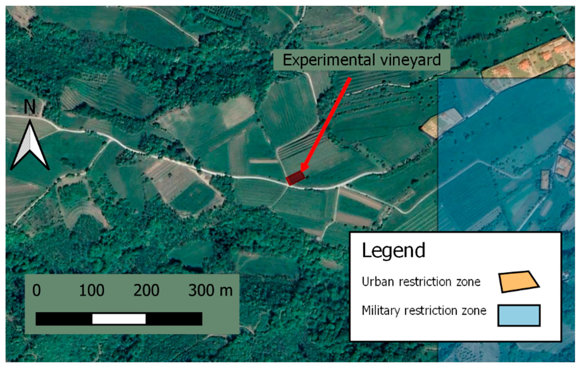
Figure 2.
Lidar and UAS survey area 28 m × 7 m (4 vine rows) and the distribution of GCPs and MTPs. The GCPs were fixed on the ground between the vine rows and the MTPs were fixed at the top of the vine rows.
Figure 2.
Lidar and UAS survey area 28 m × 7 m (4 vine rows) and the distribution of GCPs and MTPs. The GCPs were fixed on the ground between the vine rows and the MTPs were fixed at the top of the vine rows.

Figure 3.
Positioning of the lidar with respect to the vines and numbering of the segments of the vine canopy (two vines on the whole test area). View from the beginning of the row (in the center), with lidar position and detected points on the vine. The left and right images show the canopy view and the annotations that the lidar saw on the left and right sides of the canopy as it moved through the vineyard.

Figure 4.
A (blue) section of the vineyard used for manual defoliation measurements, with local coordinate system (X, Y, Z). The green vertical poles and the red ribbon (collinear with x) can be seen; the horizontal ropes were somewhat hidden by the leaves.
Figure 4.
A (blue) section of the vineyard used for manual defoliation measurements, with local coordinate system (X, Y, Z). The green vertical poles and the red ribbon (collinear with x) can be seen; the horizontal ropes were somewhat hidden by the leaves.

Figure 5.
Representation of the calculation of vine canopy volumes of individual scans. A section of segments S13, S14, and S15 colored with yellow, blue, and red is on the left and representation of the volume calculation from multiple points within segment S14 using the trapezoidal method is on the right.

Figure 6.
The UAS surveyed experimental vineyard as a point cloud from UAS photogrammetry measurements with about 195 million points (a), and the section used for the method comparison with about 30 million points (b).
Figure 6.
The UAS surveyed experimental vineyard as a point cloud from UAS photogrammetry measurements with about 195 million points (a), and the section used for the method comparison with about 30 million points (b).

Figure 7.
Comparison of point clouds from terrestrial lidar (red) and UAS photogrammetry (blue) in a side view (right side of the canopy).
Figure 7.
Comparison of point clouds from terrestrial lidar (red) and UAS photogrammetry (blue) in a side view (right side of the canopy).

Figure 8.
Comparison of point clouds from terrestrial lidar (red) and UAS photogrammetry (blue) in a top view (right side of the canopy).
Figure 8.
Comparison of point clouds from terrestrial lidar (red) and UAS photogrammetry (blue) in a top view (right side of the canopy).

Figure 9.
Comparison of point clouds from terrestrial lidar (red) and UAS photogrammetry (blue) in a side view (left side of the canopy).
Figure 9.
Comparison of point clouds from terrestrial lidar (red) and UAS photogrammetry (blue) in a side view (left side of the canopy).

Figure 10.
Comparison of point clouds from terrestrial lidar (red) and UAS photogrammetry (blue) in a top view (left side of the canopy).
Figure 10.
Comparison of point clouds from terrestrial lidar (red) and UAS photogrammetry (blue) in a top view (left side of the canopy).

Figure 11.
Reconstruction of the canopy from lidar measurement points. Segments of the same height are shown in different colors: (a) left side of the canopy, (b) right side of the canopy.
Figure 11.
Reconstruction of the canopy from lidar measurement points. Segments of the same height are shown in different colors: (a) left side of the canopy, (b) right side of the canopy.


Figure 12.
Photogrammetric side view of canopy volume and a 3D projection at different segment subdivisions (n = 1 to n = 15) for the right half of the vine. Segments of the same height are shown in different colors.
Figure 12.
Photogrammetric side view of canopy volume and a 3D projection at different segment subdivisions (n = 1 to n = 15) for the right half of the vine. Segments of the same height are shown in different colors.

Figure 13.
Correlation between number of points in segment (lidar measurements) and leaf area in segment (manual measurements): (a) left side of canopy and (b) right side of canopy. Correlation was performed for all 12 segments.
Figure 13.
Correlation between number of points in segment (lidar measurements) and leaf area in segment (manual measurements): (a) left side of canopy and (b) right side of canopy. Correlation was performed for all 12 segments.

Figure 14.
Correlation between vine canopy volume (lidar measurements) and leaf area (manual measurements): (a) left side of vine canopy and (b) right side of vine canopy. Correlation was performed for all 12 segments.
Figure 14.
Correlation between vine canopy volume (lidar measurements) and leaf area (manual measurements): (a) left side of vine canopy and (b) right side of vine canopy. Correlation was performed for all 12 segments.

Figure 15.
Correlation between vine canopy volume (photogrammetric measurements) and leaf area (manual measurements): (a) left side of vine canopy and (b) right side of vine canopy. Correlation was performed for all 12 segments.
Figure 15.
Correlation between vine canopy volume (photogrammetric measurements) and leaf area (manual measurements): (a) left side of vine canopy and (b) right side of vine canopy. Correlation was performed for all 12 segments.

Figure 16.
Correlation between the number of points (photogrammetric measurements) and the number of points (lidar measurements): (a) left side of canopy and (b) right side of canopy. The correlation was performed for all 12 segments.
Figure 16.
Correlation between the number of points (photogrammetric measurements) and the number of points (lidar measurements): (a) left side of canopy and (b) right side of canopy. The correlation was performed for all 12 segments.

Figure 17.
Correlation between digital volume (photogrammetric measurements) and digital volume (lidar measurements): (a) left side of canopy and (b) right side of canopy. The correlation was performed for all 12 segments.
Figure 17.
Correlation between digital volume (photogrammetric measurements) and digital volume (lidar measurements): (a) left side of canopy and (b) right side of canopy. The correlation was performed for all 12 segments.


Table 1.
Summary of flight parameters for the flight missions.
| Flight Mission 1—Planned and Flown with the Pix4D Capture Application | ||||
|---|---|---|---|---|
| Height AGL (m) | Camera Angle (°) | GSD (cm/pix) | Number of Images (-) | Image Overlap (%) |
| 10 | 60 | 0.24 | 360 | 90 |
| Flight mission 2—manually planned and flown with the DJI GO 4 application | ||||
| Left canopy side (shadow) | ||||
| Height AGL (m) | Camera angle (°) | GSD (cm/pix) | Number of images (-) | Image overlap (%) |
| 4 | 32 | 0.09 | 34 | 74 |
| 6 | 47 | 0.14 | 37 | 84 |
| 8 | 56 | 0.19 | 50 | 91 |
| Right canopy side (sun) | ||||
| Height AGL (m) | Camera angle (°) | GSD (cm/pix) | Number of images (-) | Image overlap (%) |
| 8 | 56 | 0.19 | 36 | 88 |
| 6 | 47 | 0.14 | 34 | 83 |
| 4 | 32 | 0.09 | 35 | 75 |
Table 2.
Results of terrestrial lidar, UAS photogrammetry, and manual measurements for the left and right halves of the vine canopy.
Table 2.
Results of terrestrial lidar, UAS photogrammetry, and manual measurements for the left and right halves of the vine canopy.
| Left Canopy Side (Shadow) | ||||||
|---|---|---|---|---|---|---|
| Manual Defoliation Measurements | Lidar Measurements | Photogrammetric Measurements | ||||
| Segment | Leaf area (m2) | Number of Leaves (-) | Number of Points in a Cloud (-) | Volume (m3) | Number of Points in a Cloud (-) | Volume (m3) |
| S1 | 0.03 | 4 | 220 | 0.00 | 49,619 | 0.01 |
| S2 | 0.36 | 33 | 1495 | 0.04 | 147,555 | 0.04 |
| S3 | 0.27 | 37 | 886 | 0.03 | 135,637 | 0.02 |
| S4 | 0.03 | 5 | 496 | 0.01 | 59,143 | 0.01 |
| S5 | 0.27 | 30 | 1657 | 0.04 | 146,823 | 0.03 |
| S6 | 0.16 | 29 | 828 | 0.02 | 69,025 | 0.01 |
| S7 | 0.06 | 8 | 544 | 0.01 | 62,551 | 0.01 |
| S8 | 0.33 | 61 | 1505 | 0.03 | 169,873 | 0.03 |
| S9 | 0.17 | 45 | 372 | 0.01 | 56,335 | 0.01 |
| S10 | 0.00 | 2 | 376 | 0.00 | 66,550 | 0.01 |
| S11 | 0.31 | 44 | 997 | 0.03 | 103,101 | 0.02 |
| S12 | 0.15 | 33 | 243 | 0.00 | 19,846 | 0.00 |
| Right canopy side (sun) | ||||||
| Manual defoliation measurements | Lidar measurements | Photogrammetric measurements | ||||
| Segment | Leaf area (m2) | Number of leaves (-) | Number of points in a cloud (-) | Volume (m3) | Number of points in a cloud (-) | Volume (m3) |
| S13 | 0.06 | 10 | 569 | 0.02 | 45,549 | 0.02 |
| S14 | 0.59 | 75 | 1527 | 0.04 | 147,211 | 0.04 |
| S15 | 0.21 | 39 | 750 | 0.01 | 91,827 | 0.01 |
| S16 | 0.09 | 16 | 343 | 0.00 | 24,788 | 0.01 |
| S17 | 0.27 | 53 | 1202 | 0.02 | 110,339 | 0.02 |
| S18 | 0.40 | 73 | 1090 | 0.02 | 115,609 | 0.02 |
| S19 | 0.03 | 5 | 128 | 0.00 | 20,969 | 0.00 |
| S20 | 0.23 | 40 | 976 | 0.01 | 90,513 | 0.02 |
| S21 | 0.30 | 63 | 1159 | 0.03 | 116,947 | 0.03 |
| S22 | 0.04 | 10 | 409 | 0.01 | 63,008 | 0.01 |
| S23 | 0.38 | 55 | 1497 | 0.03 | 163,401 | 0.04 |
| S24 | 0.09 | 21 | 792 | 0.02 | 112,904 | 0.01 |
Publisher’s Note: MDPI stays neutral with regard to jurisdictional claims in published maps and institutional affiliations. |
© 2022 by the authors. Licensee MDPI, Basel, Switzerland. This article is an open access article distributed under the terms and conditions of the Creative Commons Attribution (CC BY) license (https://creativecommons.org/licenses/by/4.0/).
Share and Cite
MDPI and ACS Style
Petrović, I.; Sečnik, M.; Hočevar, M.; Berk, P. Vine Canopy Reconstruction and Assessment with Terrestrial Lidar and Aerial Imaging. Remote Sens. 2022, 14, 5894. https://doi.org/10.3390/rs14225894
AMA Style
Petrović I, Sečnik M, Hočevar M, Berk P. Vine Canopy Reconstruction and Assessment with Terrestrial Lidar and Aerial Imaging. Remote Sensing. 2022; 14(22):5894. https://doi.org/10.3390/rs14225894
Chicago/Turabian StylePetrović, Igor, Matej Sečnik, Marko Hočevar, and Peter Berk. 2022. "Vine Canopy Reconstruction and Assessment with Terrestrial Lidar and Aerial Imaging" Remote Sensing 14, no. 22: 5894. https://doi.org/10.3390/rs14225894
Note that from the first issue of 2016, this journal uses article numbers instead of page numbers. See further details here.