Quality Control of CyGNSS Reflectivity for Robust Spatiotemporal Detection of Tropical Wetlands

Abstract

The aim of this study was to develop a robust methodology for evaluating the spatiotemporal dynamics of the inundation status in tropical wetlands with the currently available Global Navigation Satellite System-Reflectometry (GNSS-R) data by proposing a new quality control technique called the “precision index”. The methodology was applied over the Mekong Delta, one of the most important rice-production systems comprising aquaculture areas and natural wetlands (e.g., mangrove forests, peatlands). Cyclone Global Navigation Satellite System (CyGNSS) constellation data (August 2018–December 2021) were used to evaluate the spatiotemporal dynamics of the reflectivity Γ over the delta. First, the reflectivity Γ, shape and size of each specular footprint and the precision index were calibrated at each specular point and reprojected to a 0.0045° resolution (approximately equivalent to 500 m) grid at a daily temporal resolution (Lv. 2 product); then, the results were obtained considering bias-causing factors (e.g., the velocity/effective scattering area/incidence angle). The Lv. 2 product was temporally integrated every 15 days with a Kalman smoother (+/− 14 days temporal localization with Gaussian kernel: 1σ = 5 days). By applying the smoother, the regional-annual dynamics over the delta could be clearly visualized. The behaviors of the GNSS-R reflectivity and the Advanced Land Observing Satellite-2 Phased-Array type L-band Synthetic Aperture Radar-2 quadruple polarimetric scatter signals were compared and found to be nonlinearly correlated due to the influence of the incidence angle and the effective scattering area.

1. Introduction

Global Navigation Satellite System Reflectometry (GNSS-R) data have the potential to regionalize methane (CH₄) emissions from land surface images by detecting their inundation status. Methane is an important greenhouse gas (GHG); its global warming potential over a 100-year horizon is 28 times higher than that of carbon dioxide (CO₂) [1]. In 2011, the CH₄ concentration was 1803 ppb, 150% higher than the preindustrial level, and a predominantly biogenic post-2006 increase has also been reported [2]. Concurrently, atmospheric methane’s δ¹³C_CH4 value has trended towards lighter (¹³C-depleted) values, implying a significant shift in the balance between the sources and sinks of CH₄ [3] and a greater contribution of biogenic CH₄ emission sources rather than fuel combustion to this rapid CH₄ concentration increase [2]. Several hypotheses have been postulated for the cause of this isotopic shift, and these hypotheses can be summarized as one or a combination of the following: (i) a change in the oxidative capacity of the atmosphere [4]; (ii) changes in the relative strengths of anthropogenic sources, such as land-use changes on tropical wetlands to agriculture or waste and fossil fuel emissions with an overall net effect of increasing emissions (e.g., [5]); and (iii) an increase in natural sources such as wetlands, potentially as a feedback effect from regional climatic change (e.g., [3]). Large gaps still exist between top-down and bottom-up CH₄ total global emissions calculations, with much of the uncertainty associated with the emissions of wetlands and other natural emissions categories [6,7], particularly in tropical wetlands [7,8,9].

Because CH₄ is emitted from inundated soil, which is spatiotemporally heterogeneous and has a flux pattern characterized by non-Gaussian/nonlinear behaviors [7], the appropriate evaluation of the CH₄ flux requires the monitoring of the inundation status with spatiotemporally high-resolution techniques [10]. GNSS-R data became a popular input source in microwave remote sensing techniques following the deployment of the Cyclone Global Navigation Satellite System (CyGNSS), an eight-microsatellite constellation data system [11]. Every single CyGNSS microsatellite has two left-hand circular polarization (LHCP) down-looking antennas pointing to the Earth’s surface with an inclination angle of approximately 28 degrees on either side of the satellite ground track [12].

The data can be used to globally detect the land surface inundation status almost daily with high-spatial-resolution L-band microwave signals (with estimated spatial resolutions of approximately 500–7000 m [13]) compared to common passive L-band microwave radiometers. A few studies have reported that the use of CyGNSS-based inundation maps for land surface methane emission simulations improved the representation of the CH₄ emission status compared to the results obtained using common wetland maps (e.g., simulating a greater amount of CH₄ emissions by detecting inundation under clouds/vegetation with GNSS-R data [14]).

There are several studies on the detection of inundation over wetlands with GNSS-R data e.g., [15,16,17,18,19]. However, the results in most studies remain spatiotemporally sparse. In most cases, the spatiotemporal interpolation is conducted with monthly observation datasets, or spatially interpolated with optical observation sensors e.g., [15,19]. Due to the limitations of L-band fine-spatial-resolution microwave remote sensing data like GNSS-R, there are only a few studies conducting the cross-validation of GNSS-R and L-band SARs observations [15]. Furthermore, from the perspective of the application of this study, most of the time, this sort of fine-spatial-resolution, satellite-derived wetland/inundation observation is downsampled or spatially thinned (a.k.a., superobservations) before being used in advanced simulation modeling approaches accompanied with high computation costs (e.g., coarse-spatial-resolution ensemble simulations or the use of superobservations to deal with observation error covariance in data assimilation tasks) by degrading the spatial resolution or thinning the observations (e.g., [14,20]). Due to the local heterogeneity of the inundation status and the non-Gaussian/nonlinear characteristics of the spatiotemporal CH₄ emission distribution at the local scale [7,8,9], the deterioration of the spatial resolution of data can introduce large discrepancies to the emission values obtained between the top-down approach and bottom-up approach [6,7,8,9,20]. Therefore, the regionalization of CH₄ emissions based on high-spatial-resolution L-band microwave data as a bottom-up approach still remains important [7,8,9,17]. Since most studies have used GNSS-R data for regional-scale simulations at a relatively coarse spatial resolution compared to remote sensing observations (e.g., 0.01°-resolution CyGNSS-based watermasks are downsampled to a 0.5° resolution to match the WetCHARTs simulation grid [14]), few studies have paid attention to the differences among each specular point’s footprint size (i.e., the glistening area). To rasterize each piece of specular point-scale vector data without downsampling for use in local-scale simulations, one must consider the difference among each specular point’s footprint size to use these signals in fine-spatial-resolution, local-scale simulations (e.g., 10–50 m resolution irrigation models [10]). This information would also be essential for determining the spatial localization scale to ensure efficient data assimilation by determining the spatial localization scale at each specular point and adequately addressing the spatial observation error covariance.

More fundamentally, the amount of data of a certain quality provided by the GNSS-R microsatellite constellation is still limited, and the observations are prone to being conducted sparsely in space; in addition, the incidence angle varies widely among specular points, which is known to cause biases in the microwave reflectivity observations (unlike other spatially continuous microwave remote sensing observations, such as those obtained from passive microwave radiometers or synthetic aperture radars). The local incidence angles of the Phased-Array L-band Synthetic Aperture Radar-2 (PALSAR-2) ScanSAR instruments vary from 25 to 50 degrees, while CyGNSS incidence angles vary from 0 to 70 degrees [13,17]). To prepare inundation maps based on GNSS-R data for future applications or to be assimilated into simulation models, the spatiotemporal interpolation step needs to be processed before the data can be used in applications. Therefore, an adaptive quality control method that considers the size of each specular point and depends on each specular point vector and incidence angle but does not require ad hoc parameter tuning or region-specific empirical parameterization with external data, such as the normalized differential vegetation index (NDVI) or digital elevation model (DEM) data, is essential for this robust interpolation preprocessing step. To realize this globally consistent rasterization at a fine spatial resolution, the authors have developed a precision index calibration scheme implemented while processing the raw specular vector data to rasterize data while considering the differences in incidence angles and specular points’ sizes/shapes/velocities. To compensate for the spatially sparse distribution of GNSS-R specular data, the temporal Kalman smoother is applied by using the precision index as the reciprocal observation error number in each 15-day cycle over the Mekong Delta as a demonstration; this case study area consists of double-/triple-rice-cropping systems, aquacultural ponds, mangroves and peatlands. Cross-validation with the PALSAR-2 quadruple polarimetric data (3–6 m resolution) product is also conducted, and the results are validated with ground inundation observation datasets [7,8,9,17]. The goal of this study is to demonstrate the usefulness of this quality control method by applying it to fine-spatiotemporal-resolution analyses over the Mekong Delta [i.e., (I) comparing it with a common change detection algorithm with the daily temporal resolution, (II) applying it with a 500 m rasterization with a 15-day temporal resolution, (III) and surveying the consistency with 3–6 m spatial-resolution L-band SAR backscatter intensities].

2. Materials and Methods

This study consists of (1) the introduction of the “precision index” for use in the quality control assessment of GNSS-R data; (2) a daily rasterization demonstration over the Mekong Delta based on the precision index obtained from the Lv. 2 product; (3) a demonstration of the temporal Kalman smoother over the Mekong Delta using the precision index as the reciprocal number of observation errors (Lv. 3 product); and (4) cross-validation with PALSAR-2 quadruple polarimetric data that have been preprocessed with a polarimetric decomposition method and ground observation data. A flowchart presenting the methodology of this study is illustrated in Figure 1.

2.1. Sites along with the Collection of Field Data

We prepared ground observation datasets obtained at six sites (A–E) located in six different districts: Site A, in Thot Not, Can Tho (10°10′N, 105°33′E); Site B, in Chau Thanh (10°16′N, 105°08′E); Site C, in Cho Moi (10°25′N, 105°27′E); Site D, in Thoai Son (10°16′N, 105°08′E); and Site E, in Tri Ton, An Giang (10°23′N, 105°06′E) [7,8,10,21,22,23,24,25,26,27] Figure S1. The soils at sites A–C are classified as silty clay fluvisol (a type of alluvial soil; [17]), while the soils at sites D and E are classified as sulfuric humaquepts (a type of alluvial soil [17]).

In Can Tho and An Giang, 50 farmers’ rice paddies (30 in site A, five each in sites B–E) were chosen as regions of interest (ROIs). At the center of each ROI, field water level data were collected for the supervised classification of the satellite remote sensing data with a water level gauge (daily, 10:00 AM–12:00 PM at site A) or with a HOBO CO-U20L-04 water level data logger (Onset Computer Corporation, United States; collected every 4 h at sites B–E). At the same time, we collected information about the history of field operations (e.g., fertilization and land preparation/sowing/harvesting dates) at each ROI throughout the observation period. The numbers of ROIs in the inundated/non-inundated rice paddies are described in the cited literature [10].

2.2. CyGNSS GNSS-R Datasets and Their Preprocessing Methods

All CyGNSS [10] Lv.1 Version 3.0 data observed from the first observation (August 2018) until December 2021 were downloaded from https://podaac.jpl.nasa.gov/dataset/CYGNSS_L1_V3.0 (accessed on 15 January 2022). The reflectivity (Γ) data were calibrated [28] using Equation (1):

$$\mathsf{\Gamma }\left(\theta \right)=\frac{{(4\pi )}^2(P_{DDM}-N){(R_r+R_t)}^2}{{\lambda }^2{G}_r{G}_t{P}_t}$$

(1)

where P_DDM is the maximum value of the analog power in the delay/Doppler maps (DDM), N is the noise floor related to the DDM, Rr is the receiver–specular point (SP) distance, Rt is the transmitter–SP distance, λ is the wavelength, θ is the incidence angle, Gr is the receiver antenna gain in the direction of the SP and GtPt is the transmitter equivalent isotropically radiated power (EIRP). The noise floor is computed as the mean value of the DDM subset, where the signal is absent (located above the characteristic horseshoe shape of the DDMs). The effect of the scattering area with the highest analog power in the DDM maps was used as the size of the specular point. Since the CyGNSS GPS signal integration time is fixed at 1 s, the footprint shape was inversely computed using the integration time, the velocity of the SP and the effective scattering area.

Our precision index model’s design was inspired by the spatial localization technique of common data assimilation methods such as the local ensemble transform Kalman filter or local particle filters [10]. The precision index (PI) was calibrated using the following equation in the grid covered by the SP footprint, as shown in Equation (2):

$$PI=\frac{\cos (\theta )\times GS}{sqrt(ESA)\times \exp (3.0\times {(DistSP/SemiDSP)}^2)} \propto \mathrm{ObsEr}$$

(2)

where θ is the incidence angle, GS is the grid spacing, ESA is the effective scattering area, DistSP is the distance from the center of the specular point, SemiDSP is the semidiameter of the ellipsoidal-shaped specular point, and ObsEr is the observation error (Figure 2).

Each specular point in the CyGNSS data format contains analog power in a 17 × 11 array of DDM bins [17 rows for Delay with a 0.25-chip resolution, 11 columns for Doppler with a 500-Hz resolution]. We also analyzed the analog power in the DDM by regarding the power as a probability density of a 3-dimensional histogram (representing skewness and kurtosis) as described in Equation (3) and Figure 3 by targeting 5 × 5 arrays surrounding the element containing the maximum analog power over the DDM at each specular point. If the kurtosis value was greater than 0.01, the precision index (P) zeroed out before its use to omit the noise derived from the specular effects over highly rough land surfaces.

$$\begin{gathered} \begin{array}{l}SKW\_a={{\displaystyle \sum _{i=-2}^2{\displaystyle \sum _{i=-2}^2\left(\frac{(P_{ij}-P_{00})/(TP\times 25)}{1/3+\sqrt{2}\left|(DPL\_P_{ij}-DPL\_P_{00})\right|}\right)}}}^3\\ SKW\_b={{\displaystyle \sum _{i=-2}^2{\displaystyle \sum _{i=-2}^2\left(\frac{(P_{ij}-P_{00})/(TP\times 25)}{1/3+\sqrt{2}\left[-(DPL\_P_{ij}-DPL\_P_{00})+(DLY\_P_{ij}-DLY\_P_{00})\right]}\right)}}}^3\\ \\ SKW\_c={{\displaystyle \sum _{i=-2}^2{\displaystyle \sum _{i=-2}^2\left(\frac{(P_{ij}-P_{00})/(TP\times 25)}{1/3+\sqrt{2}\left[(DPL\_P_{ij}-DPL\_P_{00})+(DLY\_P_{ij}-DLY\_P_{00})\right]}\right)}}}^3\\ \hspace{1em}\hspace{1em}\hspace{1em}\hspace{1em}DDM\_SKW=MAX\{abs(SKW\_a),abs(SKW\_b),abs(SKW\_c)\}\\ \\ DDM\_KTS={{\displaystyle \sum _{i=-2}^2{\displaystyle \sum _{i=-2}^2\left(\frac{(P_{ij}-P_{00})/(TP\times 25)}{1/3+\sqrt{2\times [{(DPL\_P_{ij}-DPL\_P_{00})}^2+{(DLY\_P_{ij}-DLY\_P_{00})}^2]}}\right)}}}^4\end{array} \end{gathered}$$

(3)

where SKW is skewness, KTS is kurtosis, $P_{00}$ is the maximum analog power value (W) on the DDM arrays of each specular point [“00” indicates the index of the element containing the maximum analog power among all arrays in the DDM; i.e., $P_{00}$ in Equation (3) is equivalent to $P_{DDM}$ in Equation (1)], $i$ and $j$ are array indexes over the DDM surrounding the maximum analog power element ($i$ is the Delay row index and $j$ is the Doppler column index), TP indicates the sum of the power analog values of all arrays in the DDM, and DPL and DLY indicate the doppler–delay index of the target element (i.e., $P_{ij}$ or $P_{00}$) over the DDM array.

After calibrating the reflectivity (Γ) and PI on a latitude/longitude map (with a 500 m resolution and a daily temporal resolution) (Lv. 2, Figure 4), the data were applied to a temporal Kalman smoother on each 15-day cycle (temporal localization scale: 14 days. 1σ = 5 days) to obtain the Lv. 3 product (Figure 5) for the subsequent spatiotemporal analysis. The Lv. 2 data were also applied for the temporal analysis (with a slight modification to the change detection algorithm described in [29]) just after being applied in the Γ(θ)-normalization task with Equation (4) and in a 30-day moving average filter; then, the results were compared with the ALOS-2/PALSAR-2 products reported in [10]. To generate the Lv. 3 products, this study simply used a linear Kalman filter (i.e., the time-evolution of the model was assumed to be negligible). Γ-reflectivity was treated as both the states and measurements.

${\mathsf{\Gamma }}_{normalized}=\frac{\mathsf{\Gamma }-{\mathsf{\Gamma }}_{\min }}{{\mathsf{\Gamma }}_{\max }-{\mathsf{\Gamma }}_{\min }}$ referring to a paper [29]

$$\mathsf{\Gamma }{(\theta )}_{normalized}=\frac{\mathsf{\Gamma }(\theta )-\mathsf{\Gamma }{(\theta )}_{\min }}{\mathsf{\Gamma }{(\theta )}_{\max }-\mathsf{\Gamma }{(\theta )}_{\min }}$$

(4)

where Γ(θ)_max/min is the temporal maximum/minimum value of the corresponding incidence angle bin. Due to the data quantity limitations of specular points obtained during the 2018–2022 period, we calibrated the incidence angle bins prepared for every 5° interval (i.e., 0–5°, 5–10°, 10–15°, 15–20°, 20–25°, 25–30°, 30–35°, 35–40°, 40–45°, 45–50°, 50–55°, 55–60°, 60–65° and 65–70° bins) in each grid.

Figure 4. A sample of the Lv. 2 daily product (a) Γ(θ)_normalized; (b) incidence angle; (c) precision index clipped at the Mekong Delta ((d) Optical image) on 4 January 2021.

Figure 4. A sample of the Lv. 2 daily product (a) Γ(θ)_normalized; (b) incidence angle; (c) precision index clipped at the Mekong Delta ((d) Optical image) on 4 January 2021.

Figure 5. A sample of the Lv. 3 15−day−cycle Kalman smoother product based on the precision index [Γ(dB) without or with applying the precision index (a,b), zeroed out based on the kurtosis threshold and DDM 3D statistics such as skewness (c) and kurtosis (d)] clipped at Mekong Delta on 1 August 2018.

Figure 5. A sample of the Lv. 3 15−day−cycle Kalman smoother product based on the precision index [Γ(dB) without or with applying the precision index (a,b), zeroed out based on the kurtosis threshold and DDM 3D statistics such as skewness (c) and kurtosis (d)] clipped at Mekong Delta on 1 August 2018.

After calibrating the reflectivity (Γ) and PI on a latitude/longitude map (with a 500 m resolution and a daily temporal resolution) (Lv. 2, Figure 4), the data were applied to a temporal Kalman smoother on each 15-day cycle (temporal localization scale: 14 days. 1σ = 5 days) to obtain the Lv. 3 product (Figure 5) for the subsequent spatiotemporal analysis. The Lv. 2 data were also applied for the temporal analysis (with a slight modification to the change detection algorithm described in [29]) just after being applied in the Γ(θ)-normalization task with Equation (4) and in a 30-day moving average filter; then, the results were compared with the ALOS-2/PALSAR-2 products reported in [10].

2.3. PALSAR-2 Datasets, Corresponding Preprocessing Methods and Cross-Validation Scheme with CyGNSS Data

PALSAR-2′s quadruple observation datasets (Lv. 1.1; 40–50 km observation widths, 70 km observation length; 307 scenes; August 2018–December 2021, Table S1) containing observations of the Mekong Delta were prepared after the radiometric and polarimetric calibration factors of the PALSAR-2 standard product were updated (on 24 March 2017 [30]). The high-spatial-resolution (4.3 m azimuthal resolution and 5.1 m range resolution at a 37° incidence angle) quadruple data were decomposed to characterize the microwave scattering pattern in inundated paddy soils and non-inundated paddy soils at different rice growth stages. The phase and polarimetry data in PALSAR-2′s quadruple observation datasets were converted into a coherency matrix; a refined Lee filter (7 × 7 window) was applied to ease speckle noise; and the data were then decomposed with Singh 7 components [31]. The digital number of the HH/HV/VH/VV microwave data was used in the backscatter reflectivity calibration expressed in Equation (5):

σ⁰ = 10·Log₁₀ < I² + Q² > − 105.0

(5)

where σ⁰ is the backscattering coefficient, I is the value of the imaginary component and Q is the value of the quadrature component of the digital numbers. The value of −105 is the calibration factor noted in the literature [30]. An inundation detection classification task (i.e., to determine whether the field water level was higher than the soil surface or not) was conducted with a support vector obtained in the previous supervised classification study [9] during ground observation collection (a total of 624 ROIs considering different rice growth stages), as mentioned above in Section 2.1. The backward geocoding of the abovementioned products was conducted by the Newton–Raphson method with ellipsoidal height data (DEM: Shuttle Radar Topography Mission 3 (SRTM3) version 4 and the EGM2008 geoid model) and the ALOS-2 orbital data (3D-spline-interpolated on every azimuth line).

The cross-validation was conducted with the PALSAR-2 preprocessed quadruple data and the CyGNSS specular points Lv. 2 data product following the calibration described in Section 2.2; these data were observed over the same locations as the PALSAR-2 geocoded images within ±3 days of the PALSAR-2 observation date. First, the PALSAR-2 data were spatially downsampled to a 500 m resolution, and then the precision index of each corresponding specular point was calibrated over the geocoded PALSAR-2 images. Finally, each weighted mean of PALSAR-2 signals (e.g., the 7-component scattering intensities, σ⁰, and the spatial inundation rate) was further weighted based on the precision index derived value over the PALSAR-2 image, and the results were compared with the CyGNSS reflectivity Γ data.

These SAR data processes were necessary for the robust validation to compensate for the footprint size difference of the inundation status that was observed between the ground point observations and the GNSS-R data that were detected from space.

3. Results

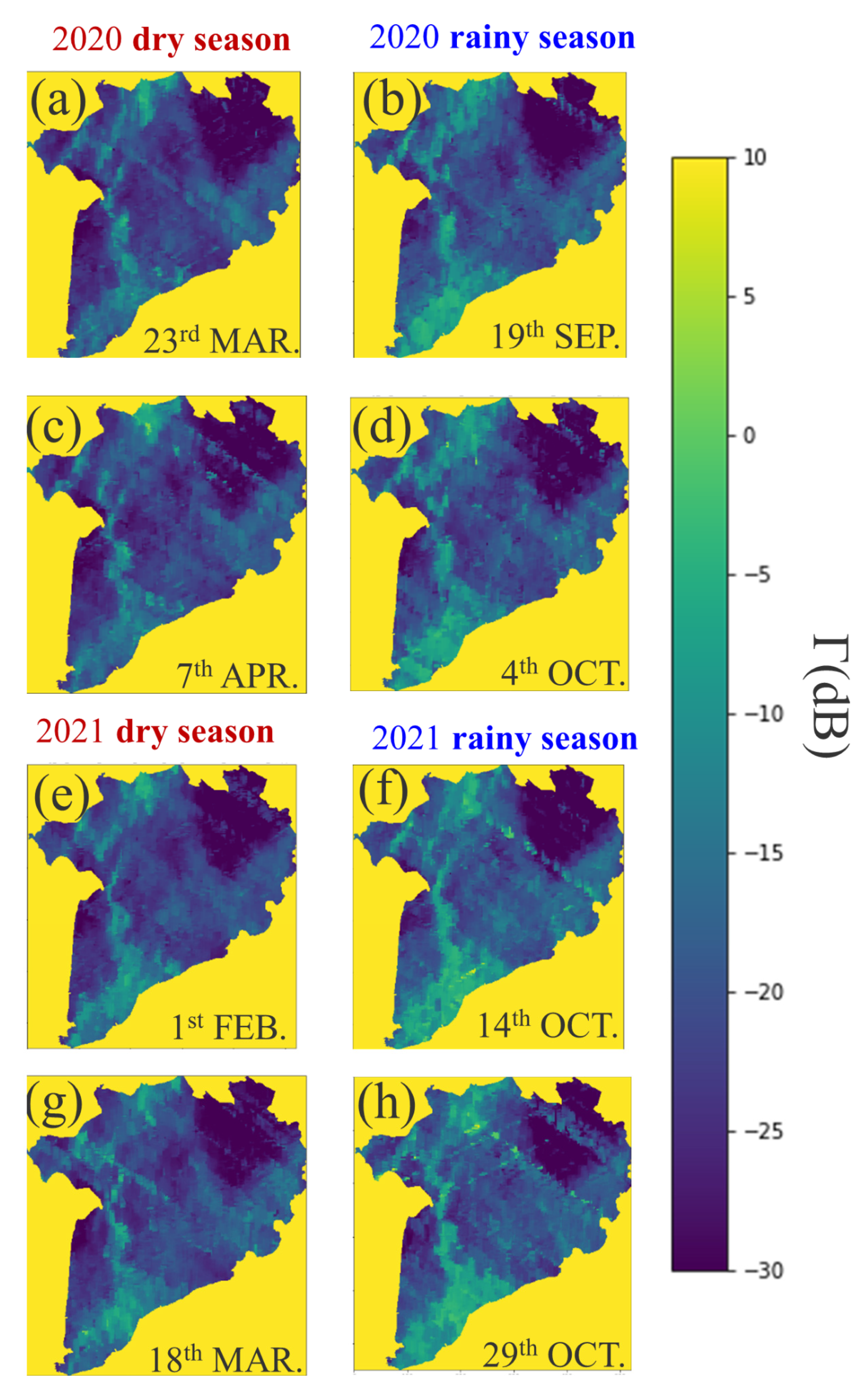
3.1. Spatiotemporal Dynamics Evaluation over the Mekong Delta by CyGNSS GNSS-R Measurements

The annual/seasonal dynamics of Γ (i.e., high values in the rainy season from June to October, and low values in the dry season from February to May) could clearly be visualized in the CyGNSS GNSS-R product, as shown in Figure 6. By improving the change detection algorithm by considering the difference in the local incidence angle among each grid cell (i.e., from Γ-normalization to Γ(θ)-normalization), two peaks with high Γ values could be detected annually.

For the Lv. 2 product, a moving average was required to see the seasonal dynamics. However, this seasonal pattern was clearly illustrated in the Lv. 3 product even if the change detection algorithm was not applied (Figure 6e). Particularly for high incidence angles (>55°), the non-normalized Γ series shows a wide distribution among relatively high dB values (−20>) during the rainy season. This indicated that our proposed precision index worked adequately as a Kalman smoother weight-mean processing tool and enabled robust spatiotemporal comparisons. Compared with the result that was obtained from the 3000 m grid spacing rasterization result without the precision index (Figure 6d), the 500 m grid spacing rasterization that was enabled by using the precision index displayed the seasonal contrast more clearly (Figure 6e).

The Γ normalization step applied to each incidence angle [i.e., Γ(θ)_normalized] significantly improved the sensitivity of the results to the temporal dynamics of the incidence angle by increasing the dynamic range [0.2–0.4 for Γ and 0.1–0.7 for Γ(θ)]. Γ(θ) values with lower incidence angles tended to show a greater dynamic range than values with higher incidence angles (Figure 6b).

The Lv. 3 product’s spatial distribution snapshot maps showed relatively strong Γ values in the northwest triple-rice-cropping region (a.k.a., Dong Thap and An Giang provinces, Figure 7). Irrespective of seasonal differences, the northeastern non-rice-cropping upland zone showed low Γ reflectivity (Figure 7). These results were consistent with the L-band SAR data-based rice paddy distribution map and rice floodability map (Figure 8 [21]). The southwestern coastal wetland zone (comprising mangrove forests, fishponds and peatlands) showed continuously high Γ values throughout the year. High Γ (dB) noise occasionally remained in the specular data in the fine-spatial-resolution (i.e., low effective scattering area) Lv. 3 product (Figure 5). However, the noise was accompanied by high DDM 3D skewness/kurtosis values because the noise was derived from the locally high land surface roughness.

3.2. Cross-Validation with PALSAR-2 Quadruple Observation Products

The relationship between CyGNSS reflectivity Γ values and PALSAR-2 backscatter σ0 values was differentiated depending on the specular point incidence angles and effective scattering area (Tables S2 and S3). Positive relationships between the Γ values and σ⁰ values were found with 0–10° incidence angles (Figures S2–S6a,b; Table S2). For specular points obtained at 10–70°, the correlations became negative, with a few exceptions observed for a fine specular point group (i.e., for incidence angles of 30–35°, the square root value of the effective scattering area is smaller than 6 km, Table S2, Figure 9). The spatial inundation rates and Γ values showed mostly positive correlations among the groups with incidence angles of 10–50°. In contrast, negative correlations tended to be dominant for low-end incidence angle groups of 0–10° and high-end incidence angle groups of 50–70° (Table S2, Figure S2). In such high-/low-end incidence angle groups, the double bounce factor tended to show the most significant co-relationship with the Γ values among the 7-component scatterings (odd/double/volume scatterings listed in Table S1 and shown in Figures S3–S5. The remaining component analysis results are not shown in this paper since the correlations were weaker than those of the odd/double/volume scatterings. In contrast, for the middle-incidence-angle groups (10–50°), the volume diffusion results tended to show the most significant correlations with the Γ values (Table S2, Figures S3–S5). Among the PALSAR-2 HH/HV/VV backscatters, HV tended to show the most significant correlations with the Γ values (Table S2, Figure S6).

The CyGNSS reflectivity Γ and PALSAR-2 backscatter data series showed a highly nonlinear relationship, and this was one of the causes of the low Pearson correlation coefficients (Table S2). Particularly for the relationship between the Γ values and the PALSAR-2-based spatial inundation percentages, three domains with unique characteristics were found (Figure S2g,m). First, for the specular points whose Γ values are approximately smaller than −20 dB, relatively high inundation percentages were found (Figure S2g,m; domain shown by the green arrow). In such a domain, the Γ values tended to show a linearly positive correlation with the inundation percentages. Second, for specular points with Γ values between approximately −20 dB and 0 dB, specular points with 0% spatial inundation percentages were detected (Figure S2g,m; domain shown by the red arrow). In this domain, the Γ values tended to correspond to upwardly convex negative nonlinear correlations. Finally, for the specular points with Γ values greater than approximately 0 dB (Figure S2g,m; domain shown by the blue arrow), relatively high inundation percentages were detected. In this domain, the Γ values tended to show upwardly convex positive nonlinear correlations.

Since the relationship between the CyGNSS reflectivity Γ and PALSAR-2 backscattering σ0 values was also highly nonlinear (Figures S3–S6), a quadratic polynomial fitting analysis was carried out to survey the direction of convexity (downwardly convex, linear, or upwardly convex; Table S3). Although the relationship was mostly downwardly convex for the groups with incidence angles of 0–60°, an upwardly convex nonlinear relationship became dominant for groups with incidence angles of 5–15° and 60–70° (Table S3, Figures S3–S6). In contrast, for the middle-incidence-angle groups (15–60°), downwardly convex nonlinear relationships represented the majority.

4. Discussion

4.1. Performance of the Precision Index in the Rasterization Process without Sacrificing Spatial Resolution

The specular point vector data derived from the Lv. 1 product were rasterized to form the Lv. 2 product, as shown in Figure 4. All the specular points depicted from southwest to northeast had relatively fine spatial resolutions due to the low effective-scattering-area values. In contrast, all the specular points depicted from northwest to southeast had relatively coarse spatial resolutions due to the relatively large effective scattering areas. It is known that the effective scattering area and footprint size/shape are mainly controlled by the Delay and Doppler effects [32]. This indicates that the relationship between the velocity (particularly in the advancing direction) of the GNSS receiver and the transmitter is the main factor controlling the spatial resolution of each specular point rather than the difference in the incidence angle or land surface roughness over lowlands such as the Mekong Delta (which has an elevation approximately 2 m above the sea surface) [21]. In this context, further GNSS-R receivers are expected to flexibly choose/adjust their transmitters to continuously receive only fine-spatial-resolution GNSS signals. The future use of geostationary GNSS transmitters or quasi-zenith-satellite-system-boarded transmitters (QZSSs) is also expected to be selected occasionally in specific regions.

The precision index developed in this study was designed to be maximized at the centers of the specular points, as the maximum analog power was detected at the center of the DDM (i.e., the neutral Delay/Doppler position), as shown in Figure 3. Since high-delay specular points are occasionally found in the Mekong Delta, hollow-ring-shaped Gaussian kernels might be appropriate for such unique specular points [32]. To further improve the index, such spatial localization regarding the dst.centerSP/semidiameter.SP ratio in the denominator of Equation (2) should be implemented for the further development of specular points with relatively high-delay chips. Considering the unique specular points for which the maximum analog power is located in the non-neutral Doppler bin, performing spatial localization while considering the specular advancing direction and Doppler effect would also be desirable, although such specular points were rarely found over the delta in this study.

The temporally Kalman-smoothed product (Lv. 3) clearly visualized the spatial pattern throughout the year, even without spatial interpolation/filtering/smoothing. This indicated that spatial inundation mapping can be accomplished even without performing a bias correction, depending on ad hoc parameter tuning to deal with incidence angle differences or even without depending on external NDVI data to deal with vegetation interactions. Although noise associated with relatively high Γ values is occasionally detected with small effective scattering specular points (Figure 5a), such specular noise was seemingly found to be accompanied by high DDM 3D skewness/kurtosis values (Figure 5c,d) and could thus be denoised naturally, as shown in Figure 5b.

4.2. Spatiotemporal Dynamics or Inundation Detection by CyGNSS

The Γ(θ) normalization results obtained for the Lv. 2 product indicated two peaks annually. The first peak was generally detected in the latter half of the dry season from April to June (Figure 6b), and the second peak was detected in the latter half of the rainy season from August to October. These findings indicate that the inundation status over the entire Mekong Delta is primarily controlled by double-/triple-rice-cropping irrigation activities. Approximately 57.4% of the rice-cropping area in 2012 was estimated to be triple-cropped [33]. Interestingly, the northwestern region where the most intensive triple rice cropping is conducted (i.e., the An Giang and Dong Thap Districts) showed significantly greater reflectivity Γ values in the rainy season than in the dry season. Interestingly, the southwestern coastal wetlands consisted of mangroves and peatlands surrounded by acid-sulfate soils [21]. The spatially high reflectivity values found in such coastal regions, even in the dry season, might have been the result of aquacultural activities, including prawn-rice cropping rotations [34]. Because the delta receives greater attention for being exposed to salinity intrusions exacerbated by rising sea levels [35], increased upstream dam construction [36] and groundwater depletion [37], further long-term observations over the delta are necessary for future assessments of the freshwater inundation status and the salinity intrusion succession status.

One of the novel features of our work that is presented in this paper is that our methodology realized the generation of spatiotemporally continuous data sets with a finer resolution (500 m spatial resolution, 15-day temporal resolution) than commonly used methods (that mostly have 3 km and 30-day resolutions, e.g., [13]), even though we did not use any spatiotemporal interpolation methods. Simple gridding without considering the size/shape of specular points cannot spatially rasterize the continuous CyGNSS GNSS-R data even with a lower resolution due to the data quantity limitation [13].

4.3. Comparison with Quadruple Polarimetric L-Band SAR Backscattering Signals

Statistically significant Pearson correlations were confirmed through the precision-index-based comparison between the CyGNSS reflectivity Γ and the PALSAR-2 backscattering intensity σ⁰ or the spatial inundation percentage. We defined the inundation status based on PALSAR-2’s 3–6 m resolution quadruple polarimetric data and ground truth observations [10]. To compensate for the spatial footprint size difference between the GNSS-R data and the inundation status observations with a finer spatiotemporal resolution in this study, we employed the product based on SAR data. There was still a discrepancy between the CyGNSS observations and the SAR-based inundation status product due to the heterogeneity surrounding the rice paddies over the Mekong Delta (e.g., buildings, forests, dykes), which was contaminated in the GNSS-R specular observations. The relationship was highly nonlinear, and its convexity was highly dependent on incidence angle differences. However, correlations were still found between these different microwave remote sensing methodologies even with the different observation resolutions over the heterogenous ground objects in this study.

As with other error-causing factors, notably, there are various factors causing geometric errors. For example, to propose a methodology that was independent from external data in this study, the ellipsoidal height that was derived from DEM and geoidal height information was not used for the rasterization process of the specular points. Most importantly, the grid-based rasterization of specular points was conducted by assuming that the velocity at each specular point was constant throughout each integration time (i.e., the acceleration of each specular point was assumed to be 0). It is still expected that the cross-validation performance could be better improved by rasterizing each specular point without the velocity-constant assumption. Regarding the geometric error correction, we also conducted a tuning experiment of the Gaussian function parameter of the precision index model [i.e., a value of 3.0 was used in this study, as described in Equation (2)] without downsampling. However, the tuning of the model parameter did not significantly differentiate the validation performance with the PALSAR-2 product (data not shown). Hence, rasterization with the consideration of acceleration was more important for tuning this model parameter. Without the acceleration information, the model tuning did not reliably improve the validation performance. For the current data interpretation, we also have to note the temporal differences between the observation times/dates of the CyGNSS and PALSAR-2 products. Due to the quantitative limitation of available specular points in this study, a low effective scattering area specular point group occasionally showed the opposite correlation with the PALSAR-2 backscatters (i.e., 30–35° incidence angles, 0–6 km square root values of the effective scattering area, Table S2). One of the causes of this result is the limited availability of quantitative specular points from CyGNSS over the Mekong Delta and the limited observable swath data of the quadruple PALSAR-2 observations (only 40–50 km widths were used to avoid incidence-angle-difference-derived biases in the polarimetric decomposition analysis). These data quantity limitations might have only partially caused the local optimization of the nonlinear function. Further observations are expected to enable the global optimization of the nonlinear function when estimating the spatial inundation percentage or backscatter intensity from CyGNSS specular reflectivity data. The most importantly, we need to reshape this gaussian function along with the specular points velocity vector (i.e., shifting the gaussian center considering the doppler frequency, and reshape the skewness regarding its delay time in DDM information [32]).

Unlike the specular points with incidence angles wider than 10°, a positive relationship was found between the CyGNSS reflectivity Γ and PALSAR-2 backscattering intensity σ⁰ series for specular points with incidence angles narrower than 10°. Since the difference between the microwave-energy-advancing vector directions of the backscatters and specular reflection values decreased as the incidence angle decreased, these positive relationships could have been found for specular points with such low incidence angles. This indicates that the reflectivity is highly dependent on the dielectric properties, particularly for low-incidence-angle specular points. Because such specular points tend to have low effective scattering areas (i.e., fine spatial resolutions), the incidence angle bias correction on such low-incidence-angle specular points is necessary to enable high-quality information on land surface properties to be derived. For most specular points with incidence angles ranging from 15 to 60°, the CyGNSS reflectivity Γ and PALSAR-2 backscatter intensity σ⁰ tended to show downwardly convex relationships (Table S3). This indicated that wetlands on relatively dry ground with a relatively low dielectric constant do not activate multi-time scattering (e.g., the double/triple bounce effect). Hence, the negative correlations between Γ values and σ⁰ values tended to appear to be simply controlled by the specular reflection or single scattering effect. However, wetlands on wet ground, which have high dielectric constants at a certain level, also enhance multi-time scattering to emit relatively strong power levels not only oriented forwards but also backward. The specular points with incidence angles wider than 60° tended to show upwardly convex negative relationships between the CyGNSS reflectivity Γ and PALSAR-2 backscattering intensity σ⁰ series. These findings indicated that if the incidence angle was wider than a certain level, the ground-volume interactions between inundated soil and wetland vegetation would be more prone to occur than if the specular points had lower incidence angles.

The three domains classified in the 2D scatter plots between the CyGNSS reflectivity Γ values and PALSAR-2-based spatial inundation percentages indicated a microwave scattering status difference among each domain (Figure S2g,m). The specular points in the first domain with Γ values lower than approximately −20 dB (Figure S2g,m; domain shown with the green arrow) tended to reflect relatively high odd/double bounce values. This finding indicated that the ground-volume interaction between inundated soil and the land-covering vegetation in wetlands plays a dominant role in the scattering process in this domain. Because positive correlations tended to appear between the CyGNSS reflectivity Γ and spatial inundation percentage series in this domain, this domain would be more sensitive to inundation than to soil moisture. In the second domain, where the Γ values were between approximately −20 dB and 0 dB, specular points with a 0% spatial inundation percentage were detected (Figure S2g,m; domain shown with the red arrow). In this domain, the Γ values mostly showed negative correlations with the spatial inundation rate and backscattering intensities. This indicates that the multi-time scattering effect would not have played a major role in this domain. Instead, the single scattering effect would have played a major role in such dry ground areas with relatively low dielectric constants. The negative correlations also indicate the possibility that the soil moisture and the vegetation water content may have greater roles than the spatial inundation percentage in such non-inundated wetland ROIs. In the third domain, where the specular points had Γ values greater than approximately 0 dB (Figure S2g,m; domain shown with the blue arrow), the Γ values tended to become significantly high, although the PALSAR-2 backscatter intensity values (including the odd scattering and double bounce values) tended to be low. These results indicate that the contribution of multi-time scattering was negligible and that the surface roughness in this domain would also be low. The presence of a water body without vegetation would have enabled such strong specular reflection conditions under weak backscattering effects. Consistently, Arai et al. [7,8,10] also reported three similar domains from HH/HV backscatter 2D distribution plots. Thus, this might be a common characteristic of L-band active microwave scattering signals collected over tropical wetlands.

For further development, the application of a precision index to a finer-spatial-resolution GNSS-R product (e.g., the CyGNSS interferometric coherence ratio product [38]) would be desirable to improve the spatial resolution of the resulting reflectivity Γ product. Since the differentiation of multi-time scattering processes using the phase information of scattered microwaves is mandatory to improve the inundation detection performance, the Stokes vector-based pseudo-3-component decomposition approach [39] or multi-polarimetric reflectivity/phase information (e.g., HydroGNSS) also need to be addressed for use with the GNSS-R data. To prepare for a robust comparison between SAR data and such polarimetric GNSS-R data, further improvement must be made to the precision index model.

In this study, effective scattering area was employed as the footprint size for the following two reasons. The L-band SAR polarimetric decomposition study of the rice paddies revealed that the SAR backscattering intensity is mainly controlled by ground vegetation and is sensitive to both canopy structure and ground inundation status and coherence was mostly low, impeding the possibility of using polinsar approach [10,21,23]. From this study, we also detected that most of the rice paddies whose L-band SAR backscattering intensity is relatively high showed low GNSS-R reflectivity (Figure 9). This indicated that the GNSS-R signal over the lowland wetlands/rice paddy is sensitive to ground-vegetation interaction and that the reflective property is incoherent rather than coherent. In subsequent studies study, the First Fresnel zone [40] should be considered as the footprint size, particularly for non-vegetated wetlands or paddies with immature rice paddies whose number of days since sowing is shorter than three weeks.

Regarding the nonlinear relationships between the CyGNSS reflectivity Γ and PALSAR-2 backscattering intensity σ⁰ and between the CyGNSS reflectivity Γ and the inundation percentages as affected by incidence angle differences, a model parameterization scheme with an improved precision index model is desirable if both SAR data and GNSS-R data are to be used cooperatively to overcome their observation scale differences.

5. Conclusions

For the operational use of GNSS-R data for sustainable tropical wetland management, a simple quality control method was proposed in this study. Even without ad hoc parameter tuning, the proposed simple model comprising the “precision index” and DDM 3D statistics showed a fine performance in visualizing the spatiotemporal dynamics of wetlands at a fine spatiotemporal resolution (500 m spatial resolution, 15-day temporal resolution). Even without using a common change detection algorithm, the precision-index-model-based approach showed temporal dynamics similar to those obtained using a change detection algorithm. By considering the incidence angle difference, we also succeeded in improving the sensitivity and dynamic range of the change detection results. As a result, we now are able to detect two annual inundation peaks over the Mekong Delta, indicating that the multi-cropping rice system dominating this region plays a major role in controlling the inundation status of the delta. The DDM 3D statistics approach was applied to successfully denoise the locally abnormal specular points by adaptively detecting specular points collected over rough land surfaces. The comparison with L-band microwave SAR data based on the precision index showed a reasonable mutual correlation and provided knowledge of how the microwave scattering pattern is affected by the incidence angle over tropical wetlands. Further study is required with a shorter-integration-time coherence product or a polarimetric decomposition product (e.g., stokes vector) containing GNSS-R data with 1st-/2nd-order specular point velocity (e.g., acceleration) derivatives to enable more precise comparisons with L-band SAR data.

References

1. Masson-Delmotte, V.; Zhai, P.; Pirani, A.; Connors, S.L.; Péan, C.; Berger, S.; Huang, M.; Yelekci, O.; Yu, R.; Zhou, B.; et al. Climate change 2021: The physical science basis. In Contribution of Working Group I to the Sixth Assessment Report of the Intergovernmental Panel on Climate Change; Cambridge University Press: Cambridge, UK, 2021. [Google Scholar]
2. Schaefer, H.; Fletcher, S.E.M.; Veidt, C.; Lassey, K.R.; Brailsford, G.W.; Bromley, T.M.; Dlugokencky, E.J.; Michel, S.E.; Miller, J.B.; Levin, I.; et al. A 21st-century shift from fossil-fuel to biogenic methane emissions indicated by 13 CH4. Science 2016, 352, 80–84. [Google Scholar] [CrossRef] [PubMed]
3. Nisbet, E.G.; Manning, M.R.; Dlugokencky, E.J.; Fisher, R.E.; Lowry, D.; Michel, S.E.; Lund Myhre, C.; Platt, S.M.; Allen, G.; Bousquet, P.; et al. Very strong atmospheric methane growth in the 4 years 2014–2017: Implications for the Paris Agreement. Glob. Biogeochem. Cycles 2019, 33, 318–342. [Google Scholar] [CrossRef] [Green Version]
4. Rigby, M.; Montzka, S.A.; Prinn, R.G.; White, J.W.C.; Young, D.; O’Doherty, S.; Lunt, M.F.; Ganesan, A.L.; Manning, A.J.; Simmonds, P.G.; et al. Role of atmospheric oxidation in recent methane growth. Proc. Natl. Acad. Sci. USA 2017, 114, 5373–5377. [Google Scholar] [CrossRef] [PubMed] [Green Version]
5. Jackson, R.B.; Saunois, M.; Bousquet, P.; Canadelle, J.G.; Poulter, B.; Stavert, A.R.; Bergamaschi, P.; Niwa, Y.; Segers, A.; Tsuruta, A. Increasing anthropogenic methane emissions arise equally from agricultural and fossil fuel sources. Environ. Res. Lett. 2020, 15, 071002. [Google Scholar] [CrossRef]
6. Saunois, M.; Stavert, A.R.; Poulter, B.; Bousquet, P.; Canadell, J.G.; Jackson, R.B.; Raymond, P.A.; Dlugokencky, E.J.; Houweling, S.; Patra, P.K.; et al. The global methane budget 2000–2017. Earth Syst. Sci. Data 2020, 12, 1561–1623. [Google Scholar] [CrossRef]
7. Arai, H.; Takeuchi, W.; Oyoshi, K.; Nguyen, L.D.; Fumoto, T.; Inubushi, K.; Le Toan, T. Pixel-Based Evaluation of and Related Greenhouse Gas in the Integrating SAR Data and ground observation. In Remote Sensing of Agriculture and Land Cover/Land Use Changes in South and Southeast Asian Countries; Springer: Cham, Switzerland, 2021; pp. 251–266. [Google Scholar]
8. Arai, H.; Takeuchi, W.; Oyoshi, K.; Nguyen, L.D.; Tachibana, T.; Uozumi, R.; Terasaki, K.; Miyoshi, T.; Yashiro, H.; Inubushi, K. Low cost and transparent MRV system of GHG emissions based on satellite remote sensing data: Case study on CH4 emission from the Mekong delta. In Monitoring of Global Environment and Disaster Risk Assessment from Space: The IIS Forum Proceedings; Volume 27 (National Diet Library, Japan) pp. 3–10. Available online: https://cir.nii.ac.jp/crid/1520853833371853952 (accessed on 10 February 2022).
9. France, J.L.; Fisher, R.E.; Lowry, D.; Allen, G.; Andrade, M.F.; Bauguitte, S.J.B.; Bower, K.; Broderick, T.J.; Daly, M.C.; Forster, G.; et al. δ13C methane source signatures from tropical wetland and rice field emissions. Phil. Trans. R. Soc. A 2021, 380, 20200449. [Google Scholar]
10. Arai, H.; Le Toan, T.; Takeuchi, W.; Oyoshi, K.; Fumoto, T.; Inubushi, K. Evaluating irrigation status in Mekong Delta through polarimetric L-band SAR data assimilation. Remote Sens. Environ. 2022, 279, 113139. [Google Scholar] [CrossRef]
11. Ruf, C.S.; Atlas, R.; Chang, P.S.; Clarizia, M.P.; Garrison, J.L.; Gleason, S.; Katzberg, S.J.; Jelenak, Z.; Johnson, J.T.; Majumdar, S.J.; et al. New Ocean Winds Satellite Mission to Probe Hurricanes and Tropical Convection. Bull. Am. Meteorol. Soc. 2016, 97, 385–395. [Google Scholar] [CrossRef]
12. Carreno-Luengo, H.; Luzi, G.; Crosetto, M. Impact of the Elevation Angle on CYGNSS-R Bistatic Reflectivity as a function of the Effective Surface Roughness Over Land Surfaces. Remote Sens. 2018, 10, 1749. [Google Scholar] [CrossRef] [Green Version]
13. Stilla, D.; Zribi, M.; Pierdicca, N.; Baghdadi, N.; Huc, M. Desert Roughness Retrieval Using CYGNSS GNSS-R Data. Remote Sens. 2020, 12, 743. [Google Scholar] [CrossRef] [Green Version]
14. Gerlein-Safdi, C.; Bloom, A.A.; Plant, G.; Kort, E.A.; Ruf, C.S. Improving representation of tropical wetland methane emissions with CYGNSS inundation maps. Glob. Biogeochem. Cycles 2021, 35, e2020GB006890. [Google Scholar] [CrossRef]
15. Rodriguez-Alvarez, N.; Podest, E.; Jensen, K.; McDonald, K.C. Classifying inundation in a tropical wetlands complex with GNSS-R. Remote Sens. 2019, 11, 1053. [Google Scholar] [CrossRef] [Green Version]
16. Zuffada, C.; Chew, C.; Nghiem, S.V. Global navigation satellite system reflectometry (GNSS-R) algorithms for wetland observations. In Proceedings of the 2017 IEEE International Geoscience and Remote Sensing Symposium (IGARSS), Fort Worth, TX, USA, 23–28 July 2017; pp. 1126–1129. [Google Scholar]
17. Chew, C.; Small, E. Estimating inundation extent using CYGNSS data: A conceptual modeling study. Remote Sens. Environ. 2020, 246, 111869. [Google Scholar] [CrossRef]
18. Setti, P.D.T.; Tabibi, S.; Van Dam, T. CYGNSS GNSS-R Data for Inundation Monitoring in the Brazilian Pantanal Wetland. In Proceedings of the IGARSS 2022-2022 IEEE International Geoscience and Remote Sensing Symposium, Kuala Lumpur, Malaysia, 17–22 July 2022; pp. 5531–5534. [Google Scholar]
19. Yang, W.; Gao, F.; Xu, T.; Wang, N.; Tu, J.; Jing, L.; Kong, Y. Daily Flood Monitoring Based on Spaceborne GNSS-R Data: A Case Study on Henan, China. Remote Sens. 2021, 13, 4561. [Google Scholar] [CrossRef]
20. Zhang, G.; Xiao, X.; Dong, J.; Zhang, Y.; Xin, F.; Qin, Y.; Doughty, R.B.; Moor, B., III. Reply to: “Correlation between paddy rice growth and satellite-observed methane column abundance does not imply causation”. Nat. Commun. 2021, 12, 1189. [Google Scholar] [CrossRef]
21. Arai, H.; Takeuchi, W.; Oyoshi, K.; Nguyen, L.D.; Inubushi, K. Estimation of Methane Emissions from Rice Paddies in the Mekong Delta Based on Land Surface Dynamics Characterization with Remote Sensing. Remote Sens. 2018, 10, 1438. [Google Scholar] [CrossRef] [Green Version]
22. Arai, H. The Anthropogenic Greenhouse Gas Emission from Tropical High Carbon Reservoirs. Chiba University Library Online Public Library Catalog. 2015. Available online: http://opac.ll.chiba-u.jp/da/curator/900119174/HMA_0068.pdf (accessed on 11 April 2018). (In Japanese).
23. Arai, H.; Takeuchi, W.; Oyoshi, K.; Nguyen, L.D.; Tachiba, T.; Inubushi, K. Regional evaluation on greenhouse gas-mitigation & yield-increase performance of a water-saving irrigation practice’s dissemination in rice paddies in the Mekong Delta. Monit. Glob. Environ. Disaster Risk Assess. Space IIS Forum Proc. 2018, 26, 43–50. [Google Scholar]
24. Van Hong, N.P.; Nga, T.T.; Arai, H.; Hosen, Y.; Chiem, N.H.; Inubushi, K. Rice straw management by farmers in a triple rice production system in the Mekong Delta, Viet Nam. Trop. Agr. Develop. 2014, 58, 155–162. [Google Scholar]
25. Arai, H.; Hosen, Y.; Van Hong, N.P.; Chiem, N.H.; Inubushi, K. Greenhouse gas emissions derived from rice straw burning and straw-mushroom cultivation in a triple rice cropping system in the Mekong Delta. Soil Sci. Plant Nutr. 2015, 61, 719–735. [Google Scholar] [CrossRef] [Green Version]
26. Arai, H.; Hosen, Y.; Chiem, N.H.; Inubushi, K. Alternate wetting and drying enhanced the yield of a triple-cropping rice paddy of the Mekong Delta. Soil Sci. Plant Nutr. 2021, 67, 493–506. [Google Scholar] [CrossRef]
27. Arai, H. Increased rice yield and reduced greenhouse gas emissions through alternate wetting and drying in a triple-cropped rice field in the Mekong Delta. Sci. Total Environ. 2022, 842, 156958. [Google Scholar] [CrossRef] [PubMed]
28. Motte, E.; Zribi, M.; Fanise, P.; Egido, A.; Darrozes, J.; Al-Yaari, A.; Baghdadi, N.; Baup, F.; Dayau, S.; Fieuzal, R.; et al. GLORI: A GNSS-R Dual Polarization Airborne Instrument for Land Surface Monitoring. Sensors 2016, 16, 732. [Google Scholar] [CrossRef] [PubMed]
29. Pierdicca, N.; Comite, D.; Camps, A.; Carreno-Luengo, H.; Cenci, L.; Clarizia, M.P.; Costantini, F.; Dente, L.; Guerriero, L.; Mollfulleda, A.; et al. Potential of spaceborne GNSS reflectometry for soil moisture, biomass and freeze-thaw monitoring: Summary of an ESA-funded study. IEEE Geosci. Remote Sens. Mag. 2021, 10, 8–38. [Google Scholar] [CrossRef]
30. Shimada, M.; Japan Aerospace Exploration Agency-Earth Observation Research Center. ALOS-2 characteristics, CAL/VAL results and operational status. In Proceedings of the ALOS Kyoto & Carbon Initiative 21th Science Team Meeting, Kyoto, Japan, 3–5 December 2014; Available online: http://www.eorc.jaxa.jp/ALOS/kyoto/dec2014_kc21/pdf/3-02_KC21_ALOS-2_Shimada-JAXA.pdf (accessed on 11 April 2018). (In Japanese).
31. Singh, G.; Malik, R.; Mohanty, S.; Rathore, V.S.; Yamada, K.; Umemura, M.; Yamaguchi, Y. Seven-component scattering power decomposition of POLSAR coherency matrix. IEEE Trans. Geosci. Remote Sens. 2019, 57, 8371–8382. [Google Scholar] [CrossRef]
32. Collett, I.W. Applying GNSS Reflectometry-Based Stare Processing to Modeling and Remote Sensing of Wind-Driven Ocean Surface Roughness. Ph.D. Thesis, University of Colorado at Boulder, Boulder, CO, USA, 2021. [Google Scholar]
33. Son, N.T.; Chen, C.F.; Chen, C.R.; Duc, H.N.; Chang, L.Y. A phenology-based classification of time-series MODIS data for rice crop monitorin in Mekong Delta, Vietnam. Remote Sens. 2013, 6, 135–156. [Google Scholar] [CrossRef] [Green Version]
34. Loc, H.H.; Lixian, M.L.; Park, E.; Dung, T.D.; Shrestha, S.; Yoon, Y.J. How the saline water intrusion has reshaped the agricultural landscape of the Vietnamese Mekong Delta, a review. Sci. Total Environ. 2021, 794, 148651. [Google Scholar] [CrossRef]
35. Le Toan, T.; Huu, N.; Simioni, M.; Phan, H.; Arai, H.; Mermoz, S.; Bouvet, A.; Eccher, I.d.; Diallo, Y.; Duong, T.H.; et al. Agriculture in Viet Nam under the impact of climate change. In Climate Change in Viet Nam. Impacts and Adaptation. A COP26 Assessment Report of the GEMMES Viet Nam Project; 2021, HAL, France. Available online: https://hal.inrae.fr/hal-03456472/file/2021_Simioni_Rapport_AFD_Climate%20change_GEMMES-pages-191-228.pdf (accessed on 1 November 2022).
36. Kondolf, G.M.; Schmitt, R.J.P.; Carling, P.A.; Goichot, M.; Keskinen, M.; Arias, M.E.; Bizzi, S.; Castelletti, A.; Cocharane, A.; Darby, S.E.; et al. Save the Mekong Delta from drowning. Science 2022, 376, 583–585. [Google Scholar] [CrossRef]
37. Minderhoud, P.S.J.; Erkens, G.; Pham, V.H.; Bui, V.T.; Erban, L.; Kooi, H.; Stouthamer, E. Impacts of 25 years of groundwater extraction on subsidence in the Mekong delta, Vietnam. Environ. Res. Lett. 2017, 12, 064006. [Google Scholar] [CrossRef]
38. Carreno-Luengo, H.; Warnock, A.; Ruf, C.S. The CYGNSS coherent End-to-end simulator: Development and results. IEEE Trans. Geosci. Remote Sens. 2022, 60, 7441–7444. [Google Scholar]
39. Bosch-Lluis, X.; Munoz-Martin, J.F.; Rodriguez-Alvarez, N.; Oudrhiri, K. Towards GNSS-R hybrid compact polarimetry: Introducing the stokes parameters for SMAP-R dataset. IEEE Trans. Geosci. Remote Sens. 2022, 60, 7425–7428. [Google Scholar]
40. Camps, A. Spatial resolution in GNSS-R under coherent scattering. IEEE Trans. Geosci. Remote Sens. 2019, 17, 32–36. [Google Scholar] [CrossRef]
Figure 1. Flowchart of the methodology of this study outlining the data, processing and analysis steps.
Remotesensing 14 05903 g001
Figure 2. Illustration of the precision index. The light blue tiles are rasterization grid cells. The yellow circular area is the effective scattering area. The red tile in the yellow/green circle effective scattering area is the corresponding grid. The green, blue and red arrows are equivalent to the GS, DistSP and SemiDSP terms in Equation (2).
Remotesensing 14 05903 g002
Figure 3. Illustration of DDM 3D statistics (skewness and kurtosis). The calibration is conducted by assuming that the analog power is equivalent to the probability density of the DDM 3D histogram (Delay, Doppler and Analogue power).
Remotesensing 14 05903 g003
Figure 6. Temporal dynamics of the Lv. 2 daily product with a 30-day moving average ((a): Γnormalized and (b): Γ(θ)normalized) and the Lv. 3 15-day-cycle Kalman smoother product [(c): Γnormalized (500 m resolution with the precision index), (d): Γ (3000 km resolution without the precision index) and e: Γ (500 m resolution without the precision index)]. Each line/plot denotes spatially averaged values over the delta.
Remotesensing 14 05903 g006
Figure 7. Samples of nonnormalized Γ values in 2020 (ad) and 2021 (eh). The left-hand side scenes are snapshots obtained in dry seasons (a,c,e,g). The right-hand side scenes are snapshots obtained in rainy seasons (b,d,f,h).
Remotesensing 14 05903 g007
Figure 8. PALSAR-2 data-based rice map ((a); white pixels indicate rice paddies), PALSAR-2 data-based rice floodability map (b) and inundation detection snapshot obtained by PALSAR-2 above one of the study sites [Thot not, Can Tho city, Vietnam, on 6 May 2016 (69 days after sowing)] with the corresponding aerial photo (c); CF: Continuously inundated paddy; AWD: Alternate wetting and drying paddy; the temporal water level dynamics of these blocks are presented in the referenced literature [21,26,27]).
Remotesensing 14 05903 g008
Figure 9. Two-dimensional scatterplots between the CyGNSS reflectivity Γ (dB) and PALSAR-2 based spatial inundation percentage (a) and PALSAR-2 back scatters σ0 (dB) values ((b) HV, (c) odd scattering, (d) volume diffusion, (e) double bounce) at specular points with 30–35° incidence angles. The statistical analysis results representing these relationships are described in Table S2.
Remotesensing 14 05903 g009
Publisher’s Note: MDPI stays neutral with regard to jurisdictional claims in published maps and institutional affiliations.