

Comparing Different Light Use Efficiency Models to Estimate the Gross Primary Productivity of a Cork Oak Plantation in Northern China
Abstract
:
1. Introduction
2. Materials and Methods
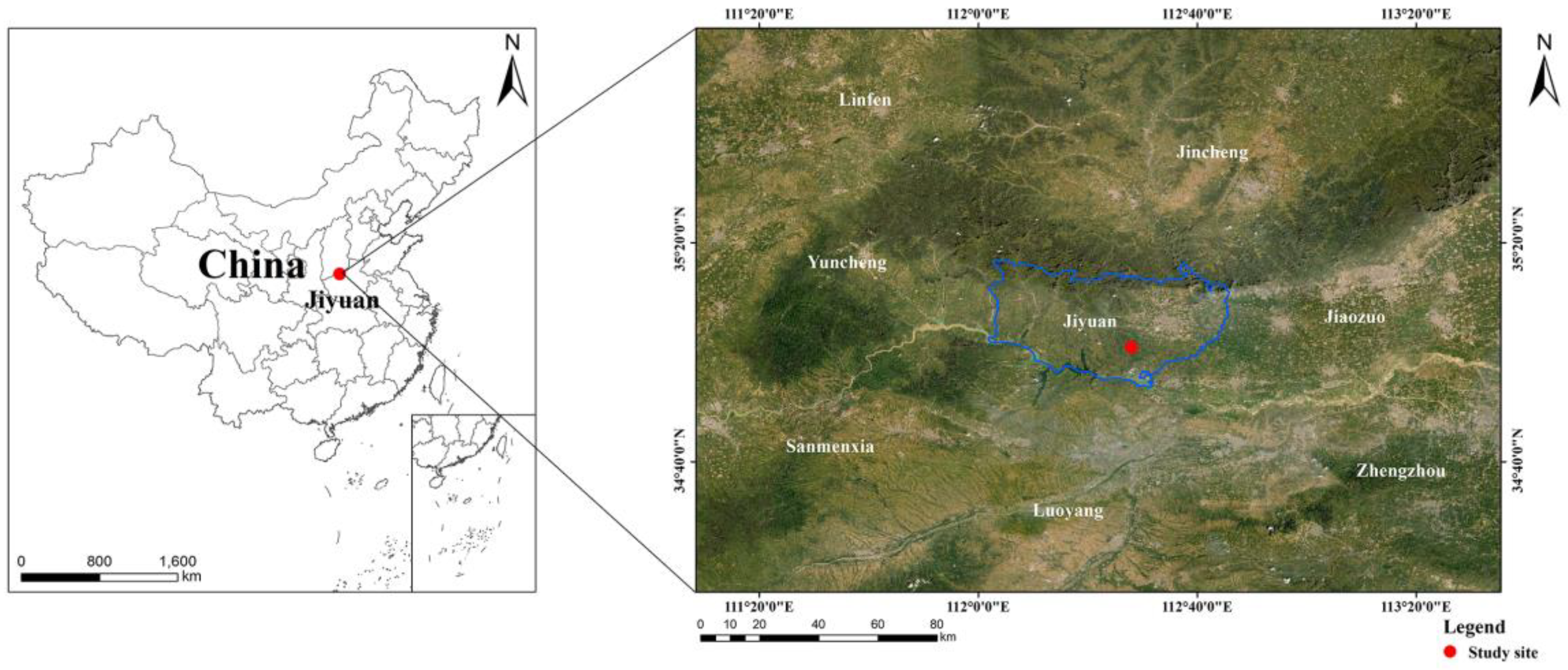
2.1. Study Area
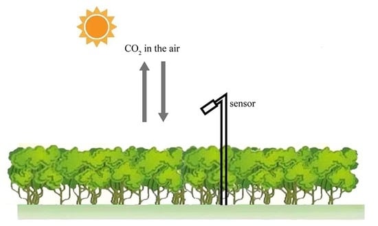
2.2. Measurements
2.3. Data Processing
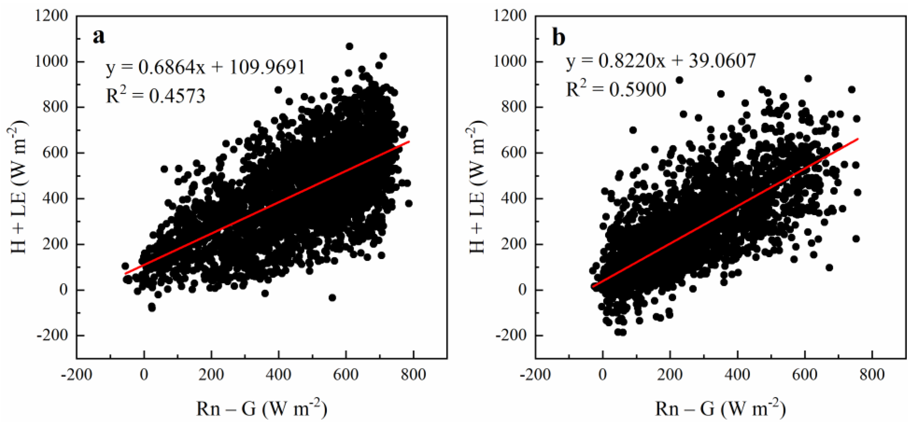
2.3.1. Fluxes Data
2.3.2. Clearness Index
2.3.3. PWSI
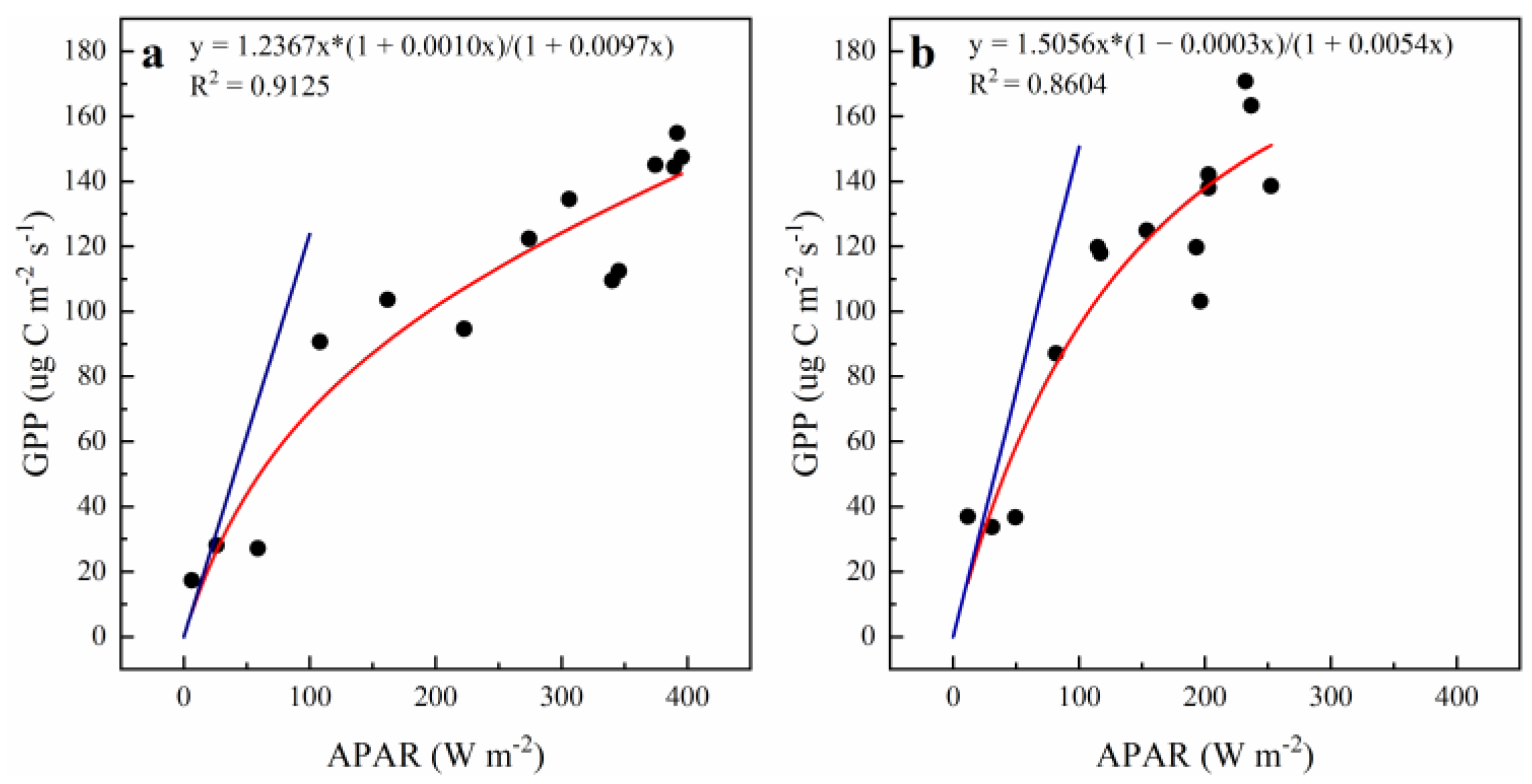
2.3.4. LUEmax
2.3.5. LUE Models
2.4. Parameter Determination
2.5. Model Performance Assessment
3. Results
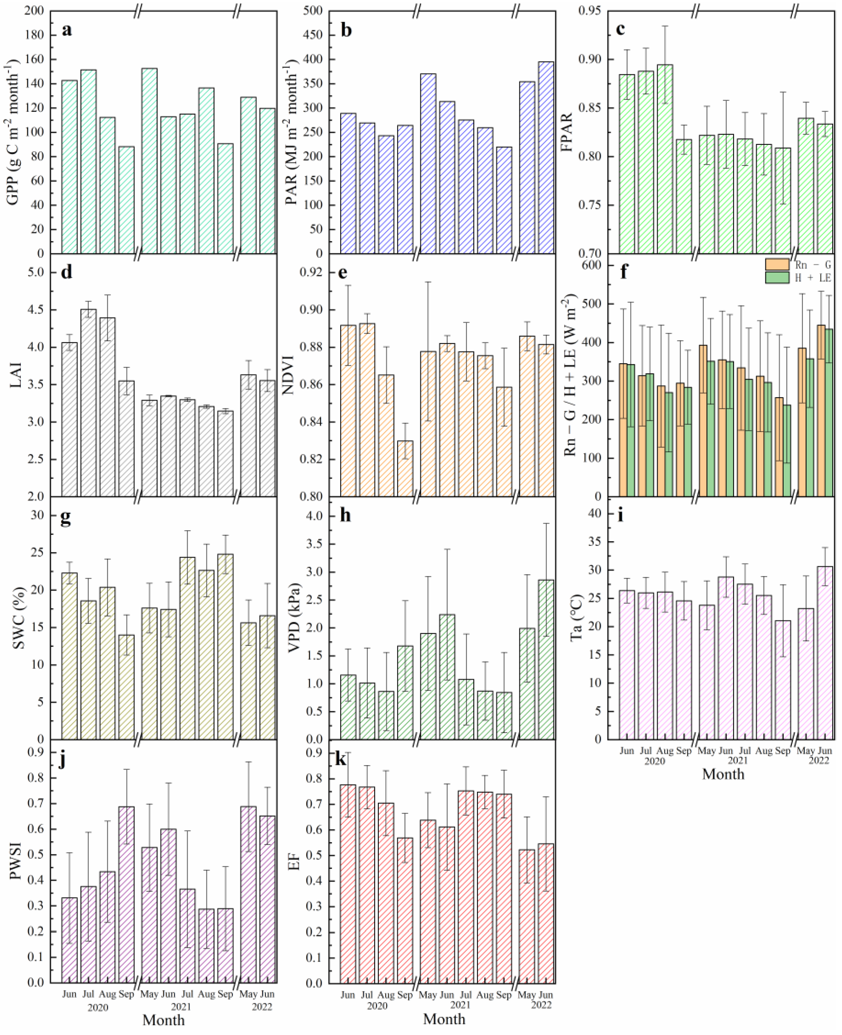
3.1. The Dynamic of GPP and Biophysical Factors during the Period of Canopy Closure
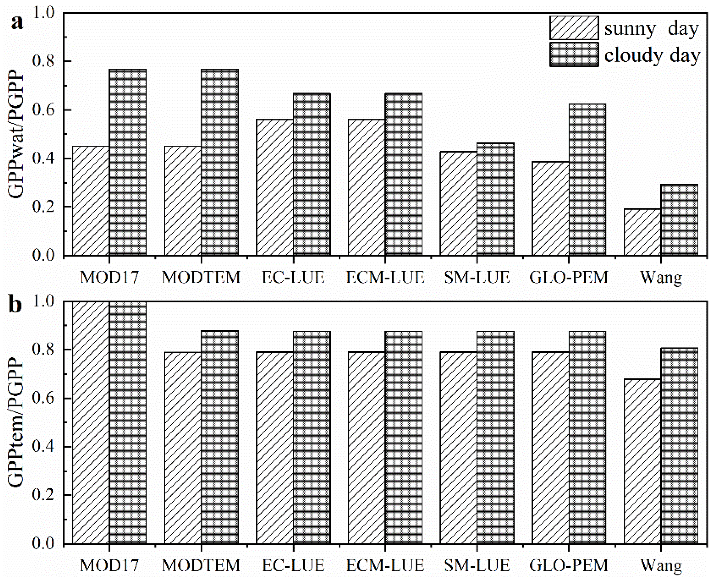
3.2. Analysis of Model Structure
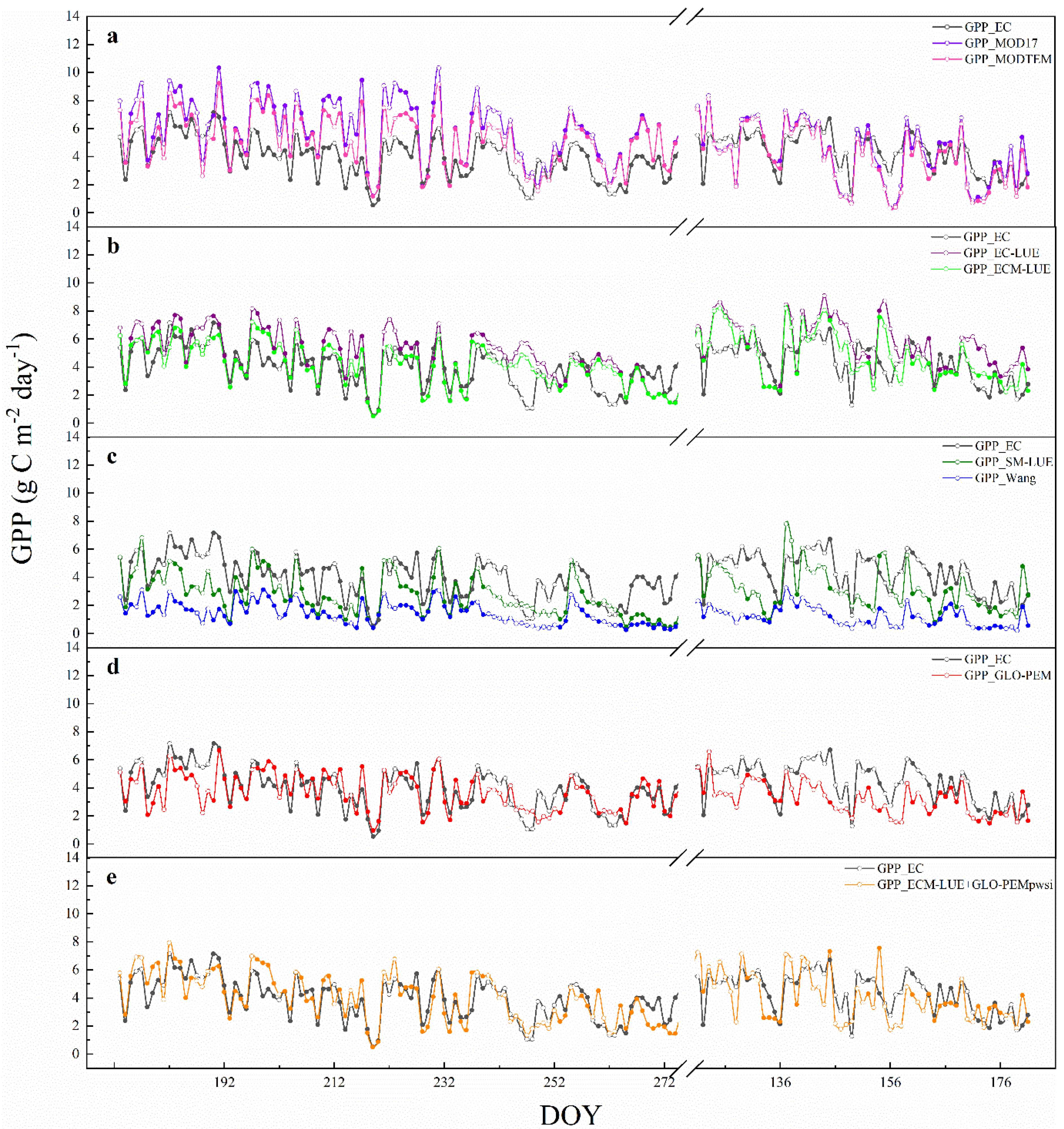
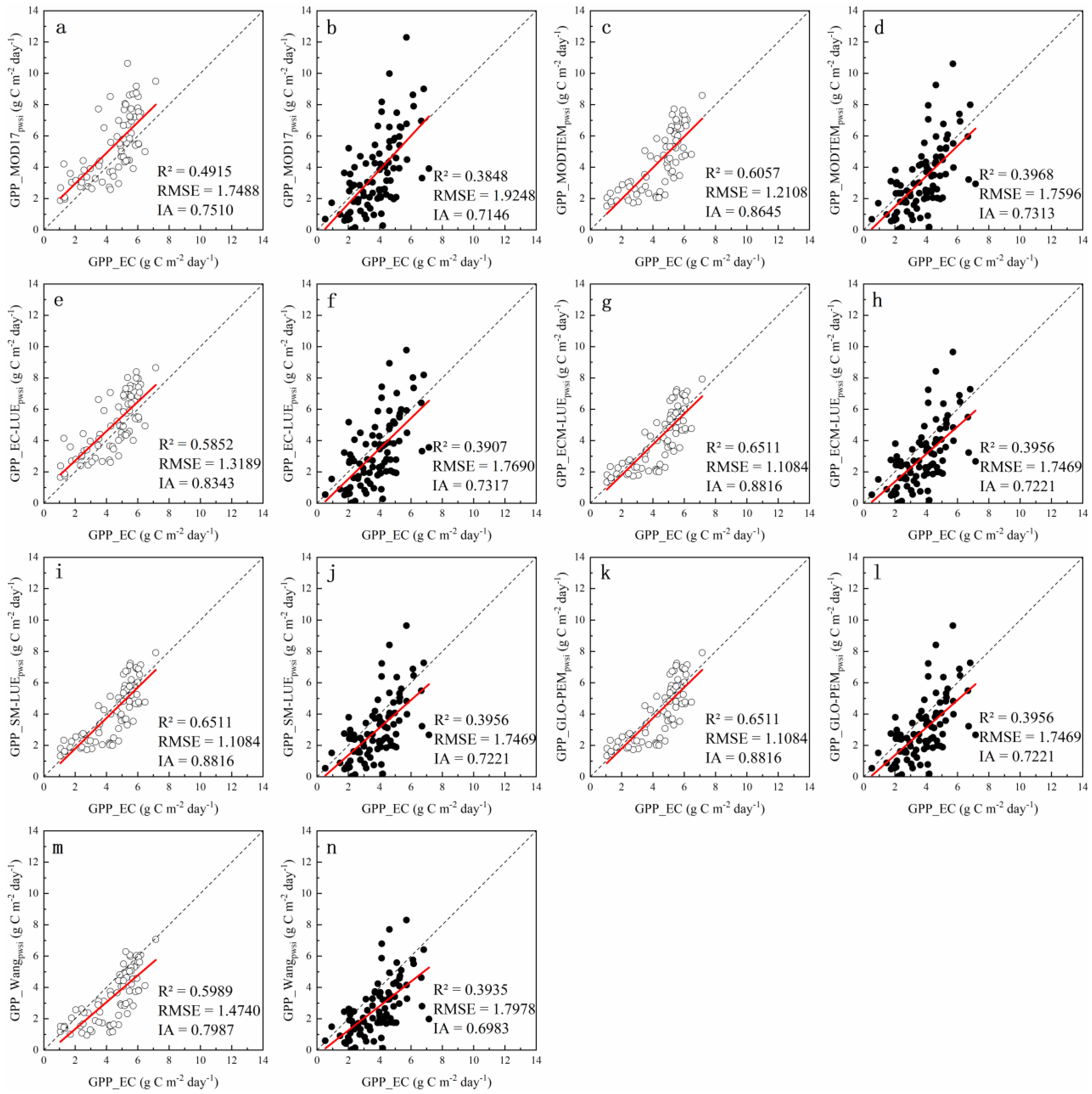
3.3. Accuracy Evaluation of Original Model
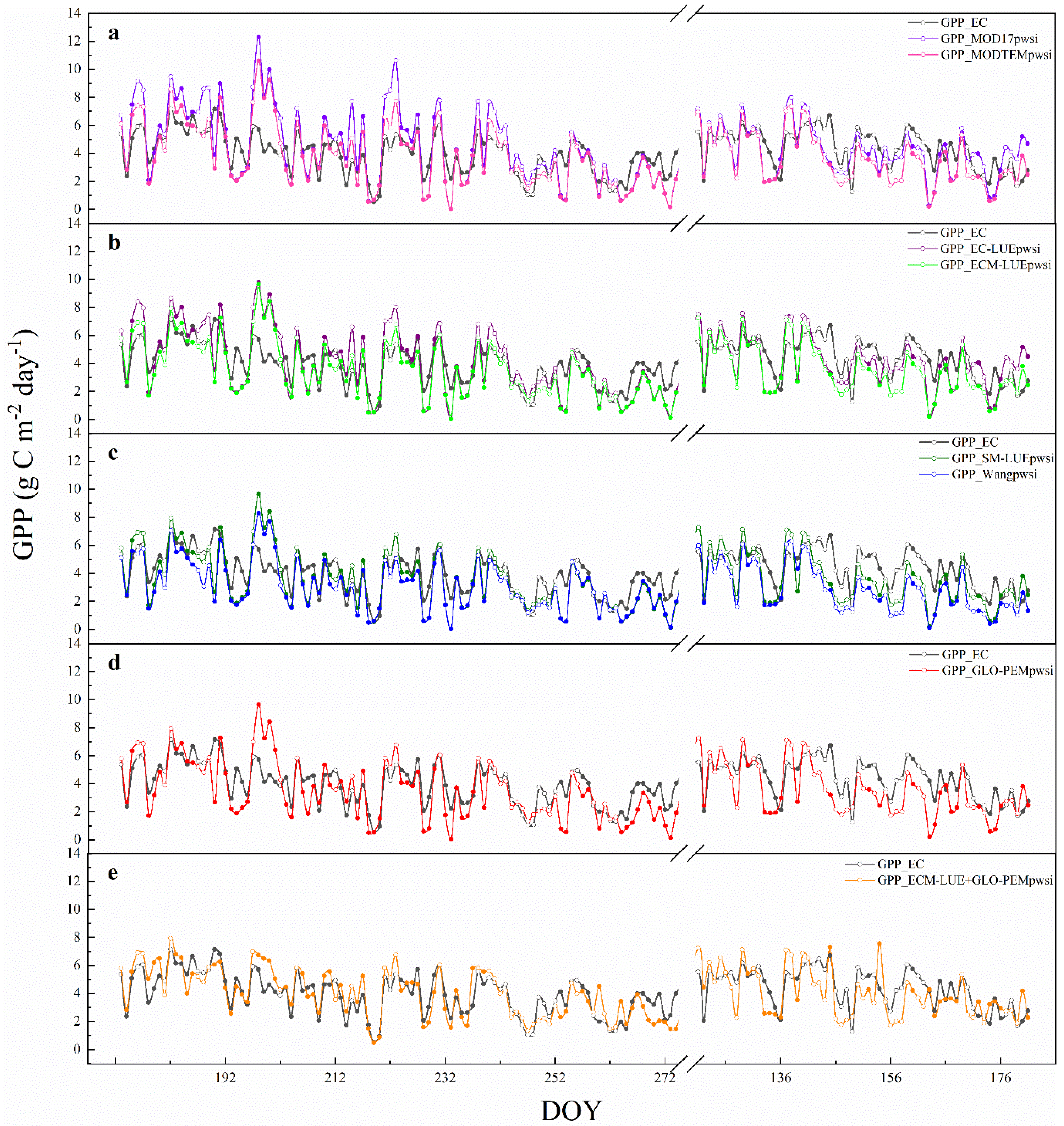
3.4. Accuracy Evaluation of Modified Model Based on PWSI
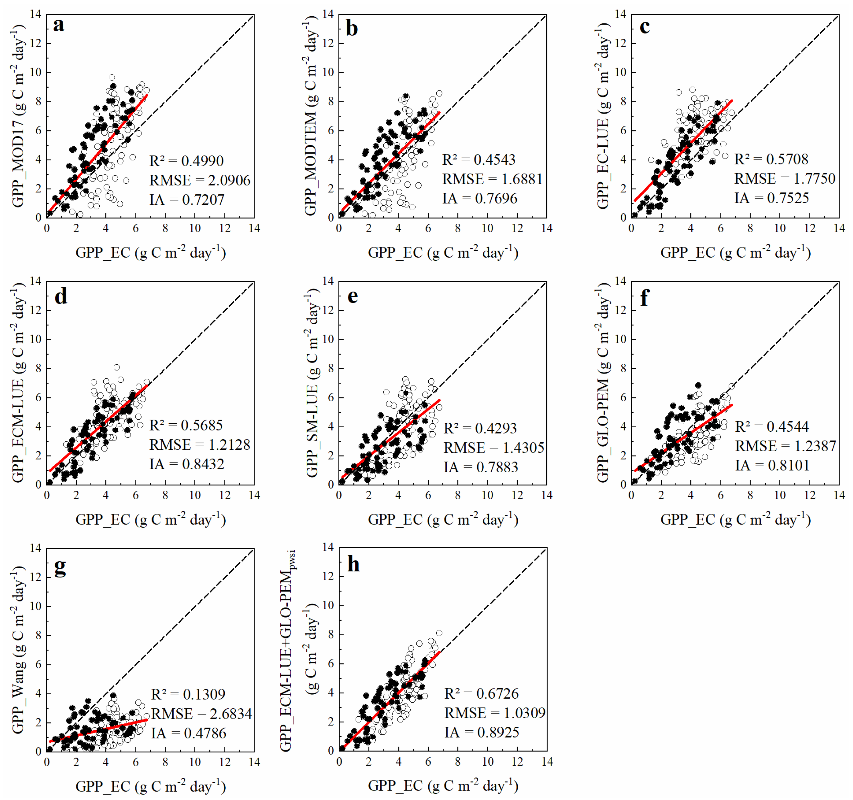
3.5. Accuracy Verification of the LUE Model with Optimal Structure
4. Discussion
5. Conclusions
Author Contributions
Funding
Data Availability Statement
Acknowledgments
Conflicts of Interest
Appendix A

References
- Trumbore, S.; Brando, P.; Hartmann, H. Forest health and global change. Science 2015, 349, 814–818. [Google Scholar] [CrossRef] [PubMed] [Green Version]
- Beer, C.; Reichstein, M.; Tomelleri, E.; Ciais, P.; Jung, M.; Carvalhais, N.; Rödenbeck, C.; Arain, M.A.; Baldocchi, D.; Bonan, G.B. Terrestrial gross carbon dioxide uptake: Global distribution and covariation with climate. Science 2010, 329, 834–838. [Google Scholar] [CrossRef] [PubMed] [Green Version]
- Fernández-Martínez, M.; Vicca, S.; Janssens, I.A.; Sardans, J.; Luyssaert, S.; Campioli, M.; Chapin Iii, F.S.; Ciais, P.; Malhi, Y.; Obersteiner, M.; et al. Nutrient availability as the key regulator of global forest carbon balance. Nat. Clim. Chang. 2014, 4, 471–476. [Google Scholar] [CrossRef] [Green Version]
- Yao, Y.; Li, Z.; Wang, T.; Chen, A.; Wang, X.; Du, M.; Jia, G.; Li, Y.; Li, H.; Luo, W.; et al. A new estimation of China’s net ecosystem productivity based on eddy covariance measurements and a model tree ensemble approach. Agric. For. Meteorol. 2018, 253–254, 84–93. [Google Scholar] [CrossRef]
- Running, S.W.; Nemani, R.R.; Heinsch, F.A.; Zhao, M.; Reeves, M.; Hashimoto, H. A continuous satellite-derived measure of global terrestrial primary production. Bioscience 2004, 54, 547–560. [Google Scholar] [CrossRef]
- Yuan, W.; Liu, S.; Zhou, G.; Zhou, G.; Tieszen, L.L.; Baldocchi, D.; Bernhofer, C.; Gholz, H.; Goldstein, A.H.; Goulden, M.L.; et al. Deriving a light use efficiency model from eddy covariance flux data for predicting daily gross primary production across biomes. Agric. For. Meteorol. 2007, 143, 189–207. [Google Scholar] [CrossRef] [Green Version]
- Pei, Y.; Dong, J.; Zhang, Y.; Yuan, W.; Doughty, R.; Yang, J.; Zhou, D.; Zhang, L.; Xiao, X. Evolution of light use efficiency models: Improvement, uncertainties, and implications. Agric. For. Meteorol. 2022, 317, 108905. [Google Scholar] [CrossRef]
- Monteith, J. Solar radiation and productivity in tropical ecosystems. J. Appl. Ecol. 1972, 9, 747–766. [Google Scholar] [CrossRef] [Green Version]
- Yuan, W.; Cai, W.; Xia, J.; Chen, J.; Liu, S.; Dong, W.; Merbold, L.; Law, B.; Arain, A.; Beringer, J.; et al. Global comparison of light use efficiency models for simulating terrestrial vegetation gross primary production based on the LaThuile database. Agric. For. Meteorol. 2014, 192–193, 108–120. [Google Scholar] [CrossRef]
- Zheng, Y.; Zhang, L.; Xiao, J.; Yuan, W.; Yan, M.; Li, T.; Zhang, Z. Sources of uncertainty in gross primary productivity simulated by light use efficiency models: Model structure, parameters, input data, and spatial resolution. Agric. For. Meteorol. 2018, 263, 242–257. [Google Scholar] [CrossRef]
- Zhang, Y.; Song, C.; Sun, G.; Band, L.E.; Noormets, A.; Zhang, Q. Understanding moisture stress on light use efficiency across terrestrial ecosystems based on global flux and remote-sensing data. J. Geophys. Res. Biogeosci. 2015, 120, 2053–2066. [Google Scholar] [CrossRef]
- Zhang, L.; Zhou, D.; Fan, J.; Hu, Z. Comparison of four light use efficiency models for estimating terrestrial gross primary production. Ecol. Model. 2015, 300, 30–39. [Google Scholar] [CrossRef] [Green Version]
- Zhang, L.; Zhou, D.; Fan, J.; Guo, Q.; Chen, S.; Wang, R.; Li, Y. Contrasting the Performance of Eight Satellite-Based GPP Models in Water-Limited and Temperature-Limited Grassland Ecosystems. Remote Sens. 2019, 11, 1333. [Google Scholar] [CrossRef] [Green Version]
- Biudes, M.S.; Vourlitis, G.L.; Velasque, M.C.S.; Machado, N.G.; de Morais Danelichen, V.H.; Pavao, V.M.; Arruda, P.H.Z.; de Souza Nogueira, J. Gross primary productivity of Brazilian Savanna (Cerrado) estimated by different remote sensing-based models. Agric. For. Meteorol. 2021, 307, 108456. [Google Scholar] [CrossRef]
- Gao, D.X.; Wang, S.; Li, Y.; Wang, C.; Wei, F.L.; Fu, B.J.; Li, T. Light use efficiency of vegetation: Model and uncertainty. Acta Ecol. Sin. 2021, 41, 5507–5516. [Google Scholar] [CrossRef]
- Idso, S.B.; Jackson, R.D.; Pinter, P.J., Jr.; Reginato, R.J.; Hatfield, J.L. Normalizing the stress-degree-day parameter for environmental variability. Agric. Meteorol. 1981, 24, 45–55. [Google Scholar] [CrossRef]
- Jackson, R.D.; Idso, S.B.; Reginato, R.J.; Pinter, P.J., Jr. Canopy temperature as a crop water stress indicator. Water Resour. Res. 1981, 17, 1133–1138. [Google Scholar] [CrossRef]
- Bellvert, J.; Marsal, J.; Girona, J.; Gonzalez-Dugo, V.; Fereres, E.; Ustin, S.; Zarco-Tejada, P. Airborne Thermal Imagery to Detect the Seasonal Evolution of Crop Water Status in Peach, Nectarine and Saturn Peach Orchards. Remote Sens. 2016, 8, 39. [Google Scholar] [CrossRef] [Green Version]
- Egea, G.; Padilla-Díaz, C.M.; Martinez-Guanter, J.; Fernández, J.E.; Pérez-Ruiz, M. Assessing a crop water stress index derived from aerial thermal imaging and infrared thermometry in super-high density olive orchards. Agric. Water Manag. 2017, 187, 210–221. [Google Scholar] [CrossRef] [Green Version]
- Irmak, S.; Haman, D.Z.; Bastug, R. Determination of Crop Water Stress Index for Irrigation Timing and Yield Estimation of Corn. Agron. J. 2000, 92, 1221–1227. [Google Scholar] [CrossRef]
- Gerhards, M.; Schlerf, M.; Rascher, U.; Udelhoven, T.; Juszczak, R.; Alberti, G.; Miglietta, F.; Inoue, Y. Analysis of Airborne Optical and Thermal Imagery for Detection of Water Stress Symptoms. Remote Sens. 2018, 10, 1139. [Google Scholar] [CrossRef] [Green Version]
- Liu, N.; Deng, Z.; Wang, H.; Luo, Z.; Gutiérrez-Jurado, H.A.; He, X.; Guan, H. Thermal remote sensing of plant water stress in natural ecosystems. For. Ecol. Manag. 2020, 476, 118433. [Google Scholar] [CrossRef]
- Li, L.; Nielsen, D.C.; Yu, Q.; Ma, L.; Ahuja, L.R. Evaluating the Crop Water Stress Index and its correlation with latent heat and CO2 fluxes over winter wheat and maize in the North China plain. Agric. Water Manag. 2010, 97, 1146–1155. [Google Scholar] [CrossRef]
- Tong, X.; Mu, Y.; Zhang, J.; Meng, P.; Li, J. Water stress controls on carbon flux and water use efficiency in a warm-temperate mixed plantation. J. Hydrol. 2019, 571, 669–678. [Google Scholar] [CrossRef]
- Barbagallo, S.; Consoli, S.; Russo, A. A one-layer satellite surface energy balance for estimating evapotranspiration rates and crop water stress indexes. Sensors 2009, 9, 1–21. [Google Scholar] [CrossRef] [Green Version]
- Berni, J.A.J.; Zarco-Tejada, P.J.; Sepulcre-Cantó, G.; Fereres, E.; Villalobos, F. Mapping canopy conductance and CWSI in olive orchards using high resolution thermal remote sensing imagery. Remote Sens. Environ. 2009, 113, 2380–2388. [Google Scholar] [CrossRef]
- Veysi, S.; Naseri, A.A.; Hamzeh, S.; Bartholomeus, H. A satellite based crop water stress index for irrigation scheduling in sugarcane fields. Agric. Water Manag. 2017, 189, 70–86. [Google Scholar] [CrossRef]
- Kanniah, K.D.; Beringer, J.; North, P.; Hutley, L. Control of atmospheric particles on diffuse radiation and terrestrial plant productivity: A review. Progr. Phys. Geogr. 2012, 36, 209–237. [Google Scholar] [CrossRef]
- Tong, X.; Zhang, J.; Meng, P.; Li, J.; Zheng, N. Light use efficiency of a warm-temperate mixed plantation in north China. Int. J. Biometeorol. 2017, 61, 1607–1615. [Google Scholar] [CrossRef]
- Xiao, X.; Zhang, Q.; Saleska, S.; Hutyra, L.; De Camargo, P.; Wofsy, S.; Frolking, S.; Boles, S.; Keller, M.; Moore, B. Satellite-based modeling of gross primary production in a seasonally moist tropical evergreen forest. Remote Sens. Environ. 2005, 94, 105–122. [Google Scholar] [CrossRef]
- Xiao, X.; Zhang, Q.; Braswell, B.; Urbanski, S.; Boles, S.; Wofsy, S.; Moore III, B.; Ojima, D. Modeling gross primary production of temperate deciduous broadleaf forest using satellite images and climate data. Remote Sens. Environ. 2004, 91, 256–270. [Google Scholar] [CrossRef]
- Liu, Z. Soil and water conservation survey in China and its application. Sci. Soil Water Conserv. 2013, 11, 1–5. [Google Scholar] [CrossRef]
- Liu, L.; Xie, Y.; Gao, X.; Cheng, X.; Huang, H.; Zhang, J. A New Threshold-Based Method for Extracting Canopy Temperature from Thermal Infrared Images of Cork Oak Plantations. Remote Sens. 2021, 13, 5028. [Google Scholar] [CrossRef]
- Liu, L.; Gao, X.; Ren, C.; Cheng, X.; Zhou, Y.; Huang, H.; Zhang, J.; Ba, Y. Applicability of the crop water stress index based on canopy–air temperature differences for monitoring water status in a cork oak plantation, northern China. Agric. For. Meteorol. 2022, 327, 109226. [Google Scholar] [CrossRef]
- Gu, L.; Fuentes, J.D.; Shugart, H.H.; Staebler, R.M.; Black, T.A. Responses of net ecosystem exchanges of carbon dioxide to changes in cloudiness: Results from two North American deciduous forests. J. Geophys. Res. Atmos. 1999, 104, 31421–31434. [Google Scholar] [CrossRef] [Green Version]
- Li, Z.; Zhang, Q.; Li, J.; Yang, X.; Wu, Y.; Zhang, Z.; Wang, S.; Wang, H.; Zhang, Y. Solar-induced chlorophyll fluorescence and its link to canopy photosynthesis in maize from continuous ground measurements. Remote Sens. Environ. 2020, 236, 111420. [Google Scholar] [CrossRef]
- Thom, A.S.; Oliver, H.R. On Penman’s equation for estimating regional evaporation. Q. J. R. Meteorol. Soc. 1977, 103, 345–357. [Google Scholar] [CrossRef]
- Ye, Z.; Yu, Q. Comparison of a new model of light response of photosynthesis with traditional models. J. Shenyang Agric. Univ. 2007, 38, 771–775. [Google Scholar] [CrossRef]
- Prince, S.D.; Goward, S.N. Global primary production: A remote sensing approach. J. Biogeogr. 1995, 22, 815–835. [Google Scholar] [CrossRef]
- Wang, S.; Ibrom, A.; Bauer-Gottwein, P.; Garcia, M. Incorporating diffuse radiation into a light use efficiency and evapotranspiration model: An 11-year study in a high latitude deciduous forest. Agric. For. Meteorol. 2018, 248, 479–493. [Google Scholar] [CrossRef]
- Wang, Q.; Li, M.W.; Li, Q.; Chen, J.L.; Yang, X.T.; Kou, Y.B.; Zhang, J.S. Drought stress indexes of soil with different texture based on chlorophyll fluorescence parameters of Quercus variabilis seedling. Sci. Soil Water Conserv. 2021, 19, 27–32. [Google Scholar] [CrossRef]
- Chen, J.; Song, X.; Wang, Q.; Wang, K.; Zhao, Y. High Temperature Index of PSIIInactivation According to chlorophyll Fluorescence. Chin. J. Agrometeorol. 2013, 34, 563–568. [Google Scholar] [CrossRef]
- Sellers, P.; Berry, J.; Collatz, G.; Field, C.; Hall, F. Canopy reflectance, photosynthesis, and transpiration. III. A reanalysis using improved leaf models and a new canopy integration scheme. Remote Sens. Environ. 1992, 42, 187–216. [Google Scholar] [CrossRef]
- Cao, M.; Prince, S.D.; Small, J.; Goetz, S.J. Remotely Sensed Interannual Variations and Trends in Terrestrial Net Primary Productivity 1981?2000. Ecosystems 2004, 7, 233–242. [Google Scholar] [CrossRef]
- Yang, D.; Xu, X.; Xiao, F.; Xu, C.; Luo, W.; Tao, L. Improving modeling of ecosystem gross primary productivity through re-optimizing temperature restrictions on photosynthesis. Sci. Total Environ. 2021, 788, 147805. [Google Scholar] [CrossRef]
- Running, S.W.; Zhao, M. Daily GPP and Annual NPP (MOD17A2/A3) products NASA Earth Observing System MODIS Land Algorithm. MOD17 User’s Guide. 2015. Available online: https://www.ntsg.umt.edu/files/modis/MOD17UsersGuide2015_v3.pdf (accessed on 5 October 2022).
- He, M.; Ju, W.; Zhou, Y.; Chen, J.; He, H.; Wang, S.; Wang, H.; Guan, D.; Yan, J.; Li, Y. Development of a two-leaf light use efficiency model for improving the calculation of terrestrial gross primary productivity. Agric. For. Meteorol. 2013, 173, 28–39. [Google Scholar] [CrossRef]
- Sims, D.A.; Rahman, A.F.; Cordova, V.D.; Baldocchi, D.D.; Flanagan, L.B.; Goldstein, A.H.; Hollinger, D.Y.; Misson, L.; Monson, R.K.; Schmid, H.P. Midday values of gross CO2 flux and light use efficiency during satellite overpasses can be used to directly estimate eight-day mean flux. Agric. For. Meteorol. 2005, 131, 1–12. [Google Scholar] [CrossRef]
- Veroustraete, F.; Sabbe, H.; Eerens, H. Estimation of carbon mass fluxes over Europe using the C-Fix model and Euroflux data. Remote Sens. Environ. 2002, 83, 376–399. [Google Scholar] [CrossRef]
- Zhou, Y.; Wu, X.; Ju, W.; Chen, J.M.; Wang, S.; Wang, H.; Yuan, W.; Andrew Black, T.; Jassal, R.; Ibrom, A. Global parameterization and validation of a two-leaf light use efficiency model for predicting gross primary production across FLUXNET sites. J. Geophys. Res. Biogeosci. 2016, 121, 1045–1072. [Google Scholar] [CrossRef]
- Keenan, T.; Baker, I.; Barr, A.; Ciais, P.; Davis, K.; Dietze, M.; Dragoni, D.; Gough, C.M.; Grant, R.; Hollinger, D. Terrestrial biosphere model performance for inter-annual variability of land-atmosphere CO2 exchange. Glob. Change Biol. 2012, 18, 1971–1987. [Google Scholar] [CrossRef]
- Raczka, B.M.; Davis, K.J.; Huntzinger, D.; Neilson, R.P.; Poulter, B.; Richardson, A.D.; Xiao, J.; Baker, I.; Ciais, P.; Keenan, T.F. Evaluation of continental carbon cycle simulations with North American flux tower observations. Ecol. Monogr. 2013, 83, 531–556. [Google Scholar] [CrossRef] [Green Version]
- Churkina, G.; Running, S.W.; Schloss, A.L.; Intercomparison, T.P.O.T.P.N.M. Comparing global models of terrestrial net primary productivity (NPP): The importance of water availability. Glob. Change Biol. 1999, 5, 46–55. [Google Scholar] [CrossRef]
- Bassow, S.; Bazzaz, F. How environmental conditions affect canopy leaf-level photosynthesis in four deciduous tree species. Ecology 1998, 79, 2660–2675. [Google Scholar] [CrossRef]
- Cheng, X.F.; Zhou, Y.; Hu, M.J.; Wang, F.; Huang, H.; Zhang, J.S. The Links between Canopy Solar-Induced Chlorophyll Fluorescence and Gross Primary Production Responses to Meteorological Factors in the Growing Season in Deciduous Broadleaf Forest. Remote Sens. 2021, 13, 2363. [Google Scholar] [CrossRef]
- Samanta, A.; Costa, M.H.; Nunes, E.L.; Vieira, S.A.; Xu, L.; Myneni, R.B. Comment on “Drought-Induced Reduction in Global Terrestrial Net Primary Production from 2000 Through 2009”. Science 2011, 333, 1093. [Google Scholar] [CrossRef] [Green Version]
- Hashimoto, H.; Wang, W.; Milesi, C.; Xiong, J.; Ganguly, S.; Zhu, Z.; Nemani, R.R. Structural uncertainty in model-simulated trends of global gross primary production. Remote Sens. 2013, 5, 1258–1273. [Google Scholar] [CrossRef] [Green Version]
- Sims, D.A.; Brzostek, E.R.; Rahman, A.F.; Dragoni, D.; Phillips, R.P. An improved approach for remotely sensing water stress impacts on forest C uptake. Glob. Change Biol. 2014, 20, 2856–2866. [Google Scholar] [CrossRef]
- Canadell, J.; Jackson, R.; Ehleringer, J.; Mooney, H.; Sala, O.; Schulze, E.-D. Maximum rooting depth of vegetation types at the global scale. Oecologia 1996, 108, 583–595. [Google Scholar] [CrossRef]
- Schenk, H.J.; Jackson, R.B. The global biogeography of roots. Ecol. Monogr. 2002, 72, 311–328. [Google Scholar] [CrossRef]
- Yuan, W.; Zheng, Y.; Piao, S.; Ciais, P.; Lombardozzi, D.; Wang, Y.; Ryu, Y.; Chen, G.; Dong, W.; Hu, Z. Increased atmospheric vapor pressure deficit reduces global vegetation growth. Sci. Adv. 2019, 5, eaax1396. [Google Scholar] [CrossRef]
- Ma, M.; Yuan, W. Differences in Gross Primary Production on the Qinghai-Tibet Plateau. Remote Sens. Technol. Appl. 2017, 32, 406–418. [Google Scholar] [CrossRef]
- Wu, X.; Ju, W.; Zhou, Y.; He, M.; Law, B.E.; Black, T.A.; Margolis, H.A.; Cescatti, A.; Gu, L.; Montagnani, L. Performance of linear and nonlinear two-leaf light use efficiency models at different temporal scales. Remote Sens. 2015, 7, 2238–2278. [Google Scholar] [CrossRef] [Green Version]
- Mu, Q.; Zhao, M.; Heinsch, F.A.; Liu, M.; Tian, H.; Running, S.W. Evaluating water stress controls on primary production in biogeochemical and remote sensing based models. J. Geophys. Res. 2007, 112. [Google Scholar] [CrossRef] [Green Version]
- Zanotelli, D.; Montagnani, L.; Andreotti, C.; Tagliavini, M. Evapotranspiration and crop coefficient patterns of an apple orchard in a sub-humid environment. Agric. Water Manag. 2019, 226, 105756. [Google Scholar] [CrossRef]
- Tong, X.; Meng, P.; Zhang, J.; Li, J.; Zheng, N.; Huang, H. Ecosystem carbon exchange over a warm-temperate mixed plantation in the lithoid hilly area of the North China. Atmos. Environ. 2012, 49, 257–267. [Google Scholar] [CrossRef]
- Xu, X.; Cheng, Y.; Zhu, D. Simulation of Gross Primary Productivity of Moso Bamboo Forest under Drought Stress based on A Light Use Efficiency Model. Acta Agric. Univ. Jiangxiensis 2019, 41, 512–520. [Google Scholar] [CrossRef]
- Maki, M.; Ishiahra, M.; Tamura, M. Estimation of leaf water status to monitor the risk of forest fires by using remotely sensed data. Remote Sens. Environ. 2004, 90, 441–450. [Google Scholar] [CrossRef]
- Xiao, J.; Zhuang, Q.; Law, B.E.; Chen, J.; Baldocchi, D.D.; Cook, D.R.; Oren, R.; Richardson, A.D.; Wharton, S.; Ma, S. A continuous measure of gross primary production for the conterminous United States derived from MODIS and AmeriFlux data. Remote Sens. Environ. 2010, 114, 576–591. [Google Scholar] [CrossRef] [Green Version]
- Gao, B.-C. NDWI—A normalized difference water index for remote sensing of vegetation liquid water from space. Remote Sens. Environ. 1996, 58, 257–266. [Google Scholar] [CrossRef]
- Jones, H.G. Use of infrared thermometry for estimation of stomatal conductance as a possible aid to irrigation scheduling. Agric. For. Meteorol. 1999, 95, 139–149. [Google Scholar] [CrossRef]
- Gautam, D.; Pagay, V. A Review of Current and Potential Applications of Remote Sensing to Study the Water Status of Horticultural Crops. Agronomy 2020, 10, 140. [Google Scholar] [CrossRef] [Green Version]
- Gardner, B.R.; Nielsen, D.C.; Shock, C.C. Infrared Thermometry and the Crop Water Stress Index. II. Sampling Procedures and Interpretation. J. Prod. Agric. 1992, 5, 466–475. [Google Scholar] [CrossRef]
- Xu, Z.Z.; Zhou, G.S. Effects of water stress and nocturnal temperature on carbon allocation in the perennial grass, Leymus chinensis. Physiol. Plant. 2005, 123, 272–280. [Google Scholar] [CrossRef]
- Wang, G.; Zhang, X.; Li, F.; Luo, Y.; Wang, W. Overaccumulation of glycine betaine enhances tolerance to drought and heat stress in wheat leaves in the protection of photosynthesis. Photosynthetica 2010, 48, 117–126. [Google Scholar] [CrossRef]
- Pradhan, G.P.; Prasad, P.V.; Fritz, A.K.; Kirkham, M.B.; Gill, B.S. Effects of drought and high temperature stress on synthetic hexaploid wheat. Funct. Plant Biol. 2012, 39, 190–198. [Google Scholar] [CrossRef]


| Model Name | Light Absorption (APAR = FPAR*PAR) | Water Scalar (Ws) | Temperature Scalar (Ts) | Reference |
|---|---|---|---|---|
| MOD17 | FPAR = 1 − exp(−k*LAI) | Ws = 0 (VPD ≥ VPDmax), or (VPDmax − VPD)/(VPDmax − VPDmin) (VPDmin < VPD < VPDmax), or 1 (VPD ≤ VPDmin) | Ts = 0 (Tamin ≤ Tamin_min), or (Tamin − Tamin_min)/(Tamin_max − Tamin_min) (Tamin_min < Tamin < Tamin_max), or 1 (Tamin ≥ Tamin_max) | [5] |
| EC-LUE | FPAR = a*NDVI − b | Ws = EF = LE/(H + LE) | Ts = ((Ta − Tmin)*(Ta − Tmax))/((Ta − Tmin)*(Ta − Tmax) − (Ta − Topt)2) | [6] |
| SM-LUE | FPAR = a*NDVI − b | Ws = 0 (SWC ≤ SWCmin), or (SWC − SWCmin)/(SWCmax − SWCmin) (SWCmin < SWC < SWCmax), or 1 (SWC ≥ SWCmax) | Ts = ((Ta − Tmin)*(Ta − Tmax))/((Ta − Tmin)*(Ta − Tmax) − (Ta − Topt)2) | This study |
| GLO-PEM | FPAR = a*NDVI − b | Ws = Ws1*Ws2 Ws1 = 1 − 0.05SHD (0 < SHD < 15), or 0.25 (SHD > 15) Ws2 = 1 − exp(0.4219*(ΔSWC − 210.6347)) | Ts = ((Ta − Tmin)*(Ta − Tmax))/((Ta − Tmin)*(Ta − Tmax) − (Ta − Topt)2) | [7,39] |
| Wang | APAR = (PAR − PARs)*fg PARs = PAR*exp(−k*LAI/cos(SZA)) fg = fAPAR/fIPAR | Ws = Ws1*Ws2*Ws3 Ws1 = 1/(1 + VPD/1.5) Ws2 = (SWC − SWCmin)/(SWCmax − SWCmin) Ws3 = fAPAR/max(fAPAR) | Ts = 1.1814/((1 + exp(0.2*(Topt − 10 − Ta))*(1 + exp(0.3*(Ta − Topt − 10))) | [40] |
| ECM-LUE | FPAR = a*NDVI − b | Ws = EF = LE/(H + LE) | Ts = ((Ta − Tmin)*(Ta − Tmax))/((Ta − Tmin)*(Ta − Tmax) − (Ta − Topt)2) | This study |
| MODTEM | FPAR = 1 − exp(−k*LAI) | Ws = 0 (VPD ≥ VPDmax), or (VPDmax − VPD)/(VPDmax − VPDmin) (VPDmin < VPD < VPDmax), or 1 (VPD ≤ VPDmin) | Ts = ((Ta − Tmin)*(Ta − Tmax))/((Ta − Tmin)*(Ta − Tmax) − (Ta − Topt)2) | This study |
Publisher’s Note: MDPI stays neutral with regard to jurisdictional claims in published maps and institutional affiliations. |
© 2022 by the authors. Licensee MDPI, Basel, Switzerland. This article is an open access article distributed under the terms and conditions of the Creative Commons Attribution (CC BY) license (https://creativecommons.org/licenses/by/4.0/).
Share and Cite
Liu, L.; Gao, X.; Cao, B.; Ba, Y.; Chen, J.; Cheng, X.; Zhou, Y.; Huang, H.; Zhang, J. Comparing Different Light Use Efficiency Models to Estimate the Gross Primary Productivity of a Cork Oak Plantation in Northern China. Remote Sens. 2022, 14, 5905. https://doi.org/10.3390/rs14225905
Liu L, Gao X, Cao B, Ba Y, Chen J, Cheng X, Zhou Y, Huang H, Zhang J. Comparing Different Light Use Efficiency Models to Estimate the Gross Primary Productivity of a Cork Oak Plantation in Northern China. Remote Sensing. 2022; 14(22):5905. https://doi.org/10.3390/rs14225905
Chicago/Turabian StyleLiu, Linqi, Xiang Gao, Binhua Cao, Yinji Ba, Jingling Chen, Xiangfen Cheng, Yu Zhou, Hui Huang, and Jinsong Zhang. 2022. "Comparing Different Light Use Efficiency Models to Estimate the Gross Primary Productivity of a Cork Oak Plantation in Northern China" Remote Sensing 14, no. 22: 5905. https://doi.org/10.3390/rs14225905