Abstract
Airborne distributed coherent aperture radar is of great significance for expanding the detection capability of the system. However, the extra observation dimension introduced by its sparse configuration also deteriorates the performance of traditional adaptive processing in a non-uniform environment. This paper focuses on moving target detection when the system works in a clutter–jamming-coexisting environment. In order to make full use of the specific low-rank structure to reduce the requirement for training data, this paper proposes a two-stage adaptive scheme that cancels jamming and clutter separately. The proposed suppression scheme first excludes the mainlobe jamming component from the training data based on the prior clutter subspace projection and performs intra-node clutter suppression. Then, the remaining jamming is jointly canceled based on the covariance obtained with its inter-pulse mixture model. Numerical examples show that this scheme can effectively reduce the blocking effect of main lobe jamming on high-speed targets but, due to the inaccuracy of the prior subspace, there is a certain additional loss of signal-to-noise ratio for near stationary targets. The simulation also shows that the proposed scheme is equally applicable to systems with a time-varying distributed geometry.
1. Introduction
Distributed coherent aperture radar is one of the most promising directions for further improving radar detection capabilities. Unlike monostatic radar with a large aperture size, distributed radar utilizes sparsely deployed nodes with small antennae to form a virtual large aperture, leading to a farther detection range and better angular resolution. Since Lincoln Laboratory proposed the concept of distributed coherent aperture radar [1,2,3], it has become one of the most promising directions for next-generation radars.
The idea of deploying distributed radar nodes on airborne platforms has drawn increasing attention recently because of the significant improvement in system maneuverability and survivability. Moreover, the sight limitation coming from the earth’s curvature could also be effectively alleviated by the elevation of observation altitude [4], thus further exploiting the advantage in long-distance detection. Compared with ground-based distributed radar, the maneuverability of the airborne platform makes the system geometry a resource that can be optimally scheduled during task execution. Therefore, airborne distributed radar significantly extends the system’s capability boundary of distributed radar.
Most of the current research on distributed radar focuses on inter-node synchronization, signal processing, etc. In terms of inter-node synchronization, a time and frequency transfer network is one of the most common solutions to keep inter-node phase coherence, and is realized by measuring the synchronization error compared with the reference source from a master node [5,6,7] or external source [8,9]. In recent years, open-loop wireless frequency transfer was explored in [10,11,12], which is attractive to airborne applications due to its flexible configuration. Due to the geometry uncertainty of the motional nodes, research on airborne distributed radar focuses more on node position calibration. Ref. [13] compensated for the phase error from geometry mismatch via echo phase search. Refs. [14,15] achieved the configuration calibration via ground auxiliary receivers. In [16], the spatial synchronization correction of distributed radar systems was completed by exploiting the inter-platform ranging information based on direct waves. The signal for open-loop frequency transfer in [12] was also used to estimate the radial distance between nodes. As for signal processing, most of the research focused on the usage of distributed virtual aperture. The Cramer–Rao bound of distributed radar’s target localization was discussed in [17], and different estimation algorithms were proposed in [18,19,20,21]. In order to reduce the influence of synchronization error, refs. [22,23] studied the estimation of coherent parameters using target echo. On the other hand, the increased angular resolution also reduces the blocking area of the jamming signal, and the mainlobe jamming suppression based on distributed radar was studied in [24,25,26,27].
Compared with ground-based distributed radar, one of the most significant differences in airborne distributed radar is the modulated clutter caused by relative motion. When jamming and clutter coexist, the electromagnetic environment around distributed radar becomes more complex, which is one of the primary problems that need to be solved by airborne distributed radar. However, at present, most of the studies on adaptive processing for distributed radar only discuss the joint spatial cancellation for jamming, thus failing to achieve the optimal suppression for the clutter component. On the other hand, the extra freedom from the distributed geometry also increases the need for training data during adaptive processing, which greatly deteriorates the performance of traditional dimensional reduction techniques developed for monostatic airborne radars in scenarios with non-uniform clutter distribution.
This paper mainly focuses on the suppression of coexisting clutter and jamming. In order to give full play to the advantage of distributed radar sparse aperture and reduce the data dimension of joint processing, suppression is divided into intra-node clutter suppression and inter-node mainlobe interference suppression, in which, sidelobe interference is also regarded as the clutter component. The contributions of this paper can be summarized as:
- (1)
- The different decorrelation characteristics of non-target components for the distributed radar system were analyzed and demonstrated with their structural covariance matrix.
- (2)
- To take advantage of different low-rank structures, a new adaptive processing scheme based on prior clutter subspace projection was proposed to suppress clutter and jamming separately, which improves the performance when training data are insufficient.
- (3)
- To eliminate the influence of varying clutter estimation on jamming suppression, the covariance matrix for inter-node processing was obtained with the mixture model of jamming, which avoids the repeated estimation of interference characteristics.
The rest of this paper is organized as follows: Section 2 provides the signal model of airborne distributed radar. Section 3 introduces the proposed clutter jamming suppression scheme in detail. In Section 4, the performance of the proposed scheme is simulated and analyzed for specific scenarios. Section 5 and Section 6 discuss and summarize the paper.
2. Signal Model
Without a loss of generality, only the single-in multiple-out (SIMO) distributed radar is modeled in this section. Assuming that the system contains L receiving nodes equipped with the same linear array antenna of N equidistant elements, the only transmitting node transmits a total of M pulses at a constant pulse repetition frequency (PRF) within a single coherent process interval (CPI). There is a moving target and multiple interference sources sparsely distributed in the target airspace, and the target echo, ground clutter, and jamming signals are sampled by all receivers at the same time. The whole observation geometry is shown in Figure 1.
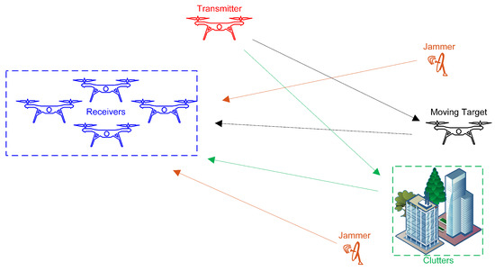
Figure 1.
System diagram of an airborne distributed coherent aperture radar operating in the scenario with active jamming.
2.1. The Compressed Echo Model in Time Domain
When working in a complex electromagnetic environment, the received signal of an array element on each distributed node is the sum of target echo, clutter, jamming, and thermal noise, i.e.,
where , , , and represent the echo component from the target, clutter, jamming, and receiver noise, respectively, and the subscripts l, m, and n denote the index of the receiving node, transmitting pulse, and array element.
Suppose that the time and frequency synchronization error between each node is negligible, and the target motion satisfies the stop-and-go model. When the range of the observation angle is much smaller than the equivalent beam width of the target, the target component after pulse compression can be expressed as:
where is the carrier frequency and represents the normalized self-correlation function of the transmitted waveform. indicates the phase difference between the transmitting node and receiving node within this CPI. denotes the constant complex scattering coefficient of the target under the coherency requirement [28]. is the propagation delay of the target, which can be approximated as (3) if the target is located in the far-field area of all array antennas, and its high-order motion relative to distributed nodes is negligible:
where c is the speed of light, and and represent the pulse repetition interval (PRI) and the adjacent spacing of array elements, respectively. is the two-way propagation delay of the target from the transmitter to the phase center of the receiver. and are the target’s two-way relative speed and azimuth. After ignoring the envelope difference caused by the angular offset and relative motion, and substituting (3) into (2), the simplified target echo can be expressed with
where represents the Doppler frequency of the target.
According to the scattering principle [4], the surface clutter can be approximated with continuously spread point scatterers, and the clutter signal can be regarded as a simple accumulation of the echoes from all clutter cells. Similar to the target, when the electrical size of the clutter cell is small enough, its scattering coefficient can also be approximated with a constant within one CPI. Thus, the clutter component of the received signal is formulated as
where superscript k is the index of clutter cells. , , and are the corresponding initial delay, Doppler frequency, and azimuth of the kth clutter cell.
Jamming signals can be classified into blocking jamming and deception jamming according to different working principles. This paper only takes noise-like blocking jamming into account. Unlike the target and clutter, the noise jamming is directly received by the receiving node after the generation and one-way free space propagation. Assuming that the jammer’s beam can cover all receivers simultaneously, the jamming component in each receiving channel has the following form:
where superscript k is the index of jammers, and represents the complex jamming envelope that varies independently between pulses. , , and are the corresponding initial delay, Doppler frequency, and azimuth of the kth jammer.
2.2. The Space-Time Steering Vector for Distributed Radar
In order to preserve the inter-node correlation of different signal components in a single range gate, the bandwidth of the transmitted signal was assumed to be narrow enough in this paper, and the envelop migration of target echo, clutter, and jamming is negligible between all receiving nodes. Generally, this requires the delay difference in each virtual aperture to be less than , where B represents the transmitting bandwidth [29]. When B is too large, the sub-band decomposition can be used to reduce the influence of envelope migration [30,31].
With the narrow band assumption, samples in different channels from the same range gate can be arranged as a column vector. For the convenience of representation, the distributed space–time steering vector, which includes the freedom degrees of array elements, is defined as
where , , , and are the delay, Doppler, azimuth, and oscillator phase vectors of the system, which contain the corresponding values of different receiving nodes. is the factor decided by the propagation delay and phase difference between the transmitter and receiver. Since the phase form transmission delay in the clutter and target components can be incorporated into the scattering coefficient, the here only contains values from receivers. is the space–time steering vector of a single array antenna, whose definition is
The above steering vectors can express target, clutter, and jamming components simultaneously. Using , , and to abbreviate, the arranged sampling vector can then be expressed as
where ⊗ and ⊙ are the Kronecker product and Hadamard product of the matrix. , , , and represent the target, clutter, jamming, and noise components, respectively. is an vector of the jamming envelope within different pulses. and are column vectors of length L and N, which are filled with 1. denotes the set of clutter cells located within the ith range gate.
2.3. The Covariance Matrix of Non-Target Components
With the sampled signal vector above, the covariance matrix of the clutter component can be expressed as:
where the is assumed to be independent between different clutter elements. Due to the structured steering vector in (7), also shares the block structure. After being divided into blocks equally, the sub-matrix of can be expressed with
where is the phase difference in the clutter cell between the th and th receiving nodes.
Since if , the diagonal sub-matrix is the same as the single-node clutter covariance matrix. On the other hand, since the distance between adjacent distributed nodes far exceeds the carrier wavelength , is modulated with a high spatial frequency along the azimuth if . Since the clutter is continuously distributed over the entire angular space, can be regarded as a complex random variable of a constant modulus whose phase is uniformly distributed between 0 and 2 pi. According to the stationary phase principle, even if the phase of is well-aligned at a specific index, the near-random modulation from would also prevent the in-phase accumulation of clutter energy, leading to a decorrelation of clutter components among different distributed nodes. Therefore, has an approximate block-diagonal structure, whose off-diagonal sub-matrices . Since all receiving nodes are equipped with the same linear array in this paper, the diagonal sub-matrix is a block Toeplitz matrix. A typical clutter covariance matrix (CCM) of airborne distributed radar is shown in Figure 2a.
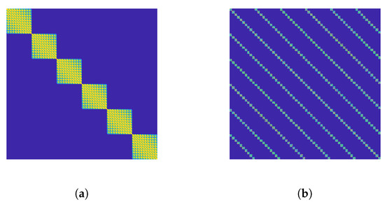
Figure 2.
The diagram of the structural covariance matrix of non-target components. (a) Clutter. (b) Block jamming.
A similar discussion on the clutter decoherence effect has been provided in [32], which models the clutter rank of airborne radar with arbitrary array geometry. Essentially, the clutter component is generated by the continuously distributed scattering surface in the scene. Although the clutter cell’s electrical size might be small enough, the overall size is far beyond the coherence limit. It should be noted that such a phenomenon does not occur in a single receiving node.
Similarly, the covariance matrix of the jamming component can be expressed with
where the independence of jamming, i.e., , has been substituted. Since the jammers are sparsely distributed in space, unlike clutter, the jamming component does not exhibit inter-node decoherence. In contrast, due to inter-pulse independence, all sub-matrices have a block-diagonal structure if is divided similarly. A typical is shown in Figure 2b.
3. The Proposed Suppression Scheme for Airborne Distributed Radar
According to the Wiener filtering theory, when the clutter, jamming, and noise components are statistically stationary, the optimal space–time beamforming vector for the signal in (9) is:
where is a covariance matrix of the non-target components. Due to the different decoherence between jamming and clutter, the optimal weight vector has different characteristics in different scenarios. When the jamming component in the echo can be ignored, the matrix degenerates into and the block-diagonal structure is restored. According to the property of the matrix inverse, is also a block-diagonal matrix, and the optimal for clutter suppression can be evenly divided into L sub-vectors
Compared with the optimal weights for monostatic clutter suppression, (14) contains an extra compensation for the inter-nodes phase change in target echoes, which reveals that the multiplied observation freedom degrees do not contribute to the overall clutter suppression ability of the system. The intra-node adaptive processing has achieved optimal clutter suppression. Similarly, the optimal jamming suppression is reduced from space–time processing to spatial because of the inter-pulse independence. The improved angular resolution narrows the adaptive spatial null, which means that inter-node processing is critical to mainlobe jamming suppression.
The different requirement on observation dimensions implies the feasibility of separating clutter and jamming suppression, i.e.,
where is a block-diagonal matrix for clutter suppression, and is the column vector for subsequent jamming cancellation. The sidelobe jamming is classified as the clutter component in the proposed scheme as it can be suppressed at the array antenna level. only performs mainlobe jamming suppression. (15) is further expanded to:
where is the block-diagonal covariance matrix for intra-node suppression. is the pulse-by-pulse beamforming matrix with a block-diagonal structure, whose definition is
where , .
Since in (16) completely removes the array dimension, the mainlobe jamming must be excluded from , as otherwise would also create a deep null in the mainlobe, suppressing the target echo and leading to beam distortion. The subsequent inter-node filtering would fail to improve the target SNR in this case because of the dimension reduction. In order to avoid under/over removal due to local fluctuations, the jamming component within the training data is estimated at the sample level and then removed, i.e.,
where denotes the original training data of the lth receiver, and represents the corresponding mainlobe jamming estimation. With , can be calculated with the estimated and then can be derived with data from all nodes.
In summary, the proposed scheme can be divided into three steps. First, each distributed node eliminates the mainlobe jamming from the training data with the aid of prior clutter subspace. Then, the CCM is estimated with preprocessed training data, and each node performs pulse-by-pulse beamforming at the target direction at the same time as clutter suppression. Finally, the suppressed data from each node are jointly processed to cancel the remaining jamming component. The data flow of the proposed scheme is shown in Figure 3, and the detailed processing in each step is discussed in the following subsections.
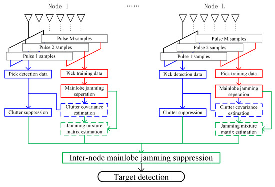
Figure 3.
The data flow of the proposed scheme.
3.1. Mainlobe Jamming Separation Based on Prior Subspace Projection
Denote the whole jamming component in as . Since the spectrum of jamming only partially overlaps with that of clutter, when contains no target echo, then should satisfy the following formula:
where the is the zero-space matrix of the monostatic CCM , i.e., . is the tolerance factor of the noise component, which determines the maximum difference between the jamming components and the training data outside the clutter subspace. Due to the inter-pulse independence of the jamming component, according to (9), the jamming component used to estimate could be expressed with the following linear combination:
where is the envelope matrix of the lth node at each training range gate. is an vector of the phase modulation with a constant modulus on shared jamming envelopes due to the relative motion between the jammer and receiver. Define the atomic set of normalized jamming components as
Then, (20) can be replaced with a linear combination of the atomic in , i.e.,
and the corresponding atomic norm can be expressed with
The atomic norm in (23) indicates the number of jammers in the whole space. Considering its sparsity, should be minimized during the jamming recovery, and the correspond estimation can be modeled as the following optimization problem:
The atomic norm minimization in (24) is non-convex and non-contiguous. Some relaxation is needed to make it easy to solve. When there is only a single mainlobe interference component, the mixing norm can be regarded as an approximation of the norm and provide a sufficient angular resolution [33]. Its corresponding convex optimization form is:
where means that the matrix on the left is positive semidefinite. is the horizontal concatenation of the column sub-matrix of , i.e.,
is a Hermitian Toeplitz matrix whose Eigen space encodes the jammers’ directions, i.e.,
is a Hermitian matrix for convex representation. It can be proven that when get minimized. The global minimization of the above semi-positive definite programming (SDP) can be efficiently calculated with a convex solver.
When there is more than one jammer within the mainlobe, the convex relaxation in (25) might fail to provide enough angler resolution and lead to an inaccurate recovery. In this case, non-convex continuous relaxation is needed to improve the resolution of the estimator. The norm re-weighting technique proposed in [34] is utilized to solve this problem, which replaces the objective function of (25) with
where is a regularization factor ised to control the non-convexity degree of the relaxation. When , (28) gradually approaches the atomic norm, whereas, if , (28) degrades to the convex relaxation in (25). Due to its concavity, any tangent plane of (28) is its upper bound, i.e.,
where is the point of tangency. After determining the initial solution, (29) can be substituted into (28), and the objective function is linear again. The minimized solution can be used as the new tangent point and update the upper bound in (29). During the iteration, the upper bound of the original objective function is continuously reduced. Thus, a local minimum of (28) is achieved. Such progress is called “majorize-minimize”. Since is a constraint for given , the optimization problem in a single iteration can be further simplified to
(25) and (30) estimate the whole jamming component, from which, the mainlobe part needs to be further separated to achieve the intended elimination. When the number of jammers in space is less than the number of array elements N, the is a non-full rank Toeplitz matrix, which means that it has a unique Vandermonde decomposition , where is a normalized Vandermonde matrix with the same rank as , and is a diagonal matrix whose values represent the amplitude ratio between different jamming signals. Since the column vectors of are the estimated jamming steering vectors in the space dimension, the components from different jammers can be decomposed into
where is a diagonal matrix whose diagonal vector is . is a column vector in which only the kth element is 1, whereas the others are 0. Since the corresponding steering vector has been obtained, the azimuth estimation could be used to judge whether is located in the mainlobe. The desired elimination in (18) could be realized by canceling the close to the beam center, i.e.,
where represents the set of jamming within the mainlobe.
The above elimination is based on the zero-space projection of the clutter covariance matrix. In practical applications, the zero-space matrix is unknown during processing. When solving (25) and (30), it needs to be replaced with the near-zero-space of a prior CCM . Since the space–time distribution of clutter is strongly correlated with the observation geometry, a with low accuracy can be obtained from the range, radar speed, yaw angle, and other information. Since (19) needs the premise that can sufficiently suppress the clutter components, it is necessary to widen the Doppler band of the CCM obtained from the geometry information to ensure that the actual clutter falls within the suppression range, which can be realized with windowing, i.e.,
where denotes the prior CCM, and is a real symmetric Toeplitz matrix.
3.2. Intra-Node Clutter Suppression
Since monostatic STAP can suppress sidelobe jamming while preserving the target energy, sidelobe jamming is equivalent to the clutter echo that continuously spreads on the whole unambiguous Doppler range at a specific angle. In order to ensure the estimation accuracy of the clutter covariance matrix with limited training data, the sub-matrix of on diagonal is estimated with contiguous sparse recovery.
Define the normalized atomic set for clutter as
Thus, the remaining non-target components in the training data can be expressed with the linear combination , and the corresponding atomic norm can be defined with
A constrained atomic norm minimization similar to (24) can be used to estimate , and the corresponding SDP during the iteration of reweighted norm relaxation is given by
Unlike (30), in (36) is a Hermitian matrix with a block Toeplitz structure. Since is an encoding matrix of the space–time distribution rather than the covariance matrix estimation, it cannot be used directly in (16). As an alternative, since the Eigen spaces of and share a similar base span, can be recovered with
where is the Eigen matrix of .
The above estimation from all nodes can then be combined into the whole CCM estimation . However, it should be noticed that the inter-pulse correlation of clutter destroys the block-diagonal structure of . As a result, although (16) performs the mainlobe beamforming pulse by pulse, the results are not inter-pulse-independent. unavoidably mixes the target echo and mainlobe jamming from different pulses. Define the mixture matrix of the intra-node suppression for a single node as ; then, the target echo and mainlobe jamming after intra-node suppression can be expressed with
3.3. Inter-Node Mainlobe Jamming Suppression
Because of the inter-pulse mixing of (38), the cancellation of mainlobe jamming cannot be achieved with a spatial filter if the mixture matrix and Doppler vector of mainlobe jamming vary among different distributed nodes. Since all pulses participate in the mixing, in theory, all of the data in CPI must be jointly processed to recover the correlation loss, i.e., STAP is still needed.
As mentioned above, the array dimension has been reduced during the intra-node suppression. The steering vector of the distributed radar after dimension reduction can be defined with
where is the mixture matrix of the whole distributed radar. is the space–time steering vector with the array dimension removed, whose definition is
Since the corrected target steering vector can be derived directly from , the key to jointly suppressing the remaining mainlobe jamming is to estimate the non-target covariance matrix after inter-pulse mixing , which is abbreviated as in this section.
Due to the local fluctuation in clutter, is not a constant in different range gates. Thus, the mainlobe jamming in (38) does not share an iso distribution. In order to improve the accuracy of , the estimation is decomposed into two parts, i.e.,
where and represent the mainlobe jamming part and non-mainlobe jamming part of , respectively.
Since is a block-diagonal matrix, can be evenly divided into sub-matrices with the definition of
Due to the inter-node clutter decorrelation, the off-diagonal only contains the sidelobe jamming, which can be ignored after intra-node suppression if the jamming energy is much higher than the noise. Thus, if . On the other hand, the on-diagonal ; thus, can be obtained with
and can be used as the estimation of .
Since the mainlobe jamming is preserved with , inter-node estimation is unavoidable for . In order to make full use of the mixture matrix , the mainlobe jamming from different directions is first separated with
where . The output covariance matrix can be formulated as
where . Here, the column vectors of are assumed to be sorted by the jammers’ angular; thus, contains only one jamming. Since and are all block-diagonal matrices, the clutter component in can be equivalent to thermal noise for jamming, i.e.,
Since does not vary within a single pulse, all of the range gates can be used for estimation. Since the clutter intensity in each range is not the same, the inverse square of the distance can be used for simple weighting. If the intra-node suppression is performed on all range gates, the clutter power can also be estimated with
and the covariance matrix of the kth jamming can be obtained by
(48) can be further corrected via rank-one approximation on the sub-slice of each pulse. The final inter-node space–time filter weights is
The complete pseudocode of the proposed adaptive suppression scheme can be summarized as Algorithm 1.
| Algorithm 1: The proposed adaptive suppression scheme. |
 |
4. Numeric Simulation
An SIMO distributed radar with receiving nodes is simulated in this section. The first node also performed as the transmitting node. All nodes were equipped with a linear array of array elements, and the adjacent element spacing was . The first node transmitted a total of pulses with a const PRF of 400 Hz. The base bandwidth MHz and the carrier frequency was MHz. The power of thermal noise was set to . Thus, the noise component in was an identity matrix.
All nodes flew at 6000 km height with a linear initial geometry parallel to the ground. The extension direction of the distributed aperture was regarded as the x-axis, and the intersection of its vertical plane and the ground surface was the y-axis. The scene’s origin was placed at the on-ground projection point of the center of the initial aperture. The target was placed on the ground surface, whose distance between the origin was 30 km. The clutter-to-noise Ratio (CNR) of the target range gate was 40 dB. The whole diagram of the simulated scene is shown in Figure 4.
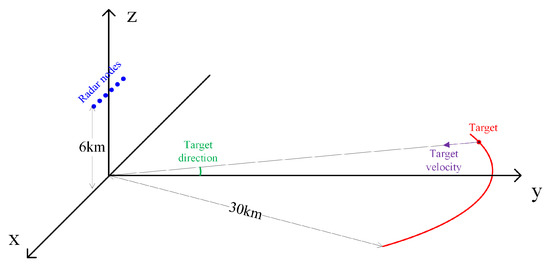
Figure 4.
Diagram of the simulated scenario with a distributed coherent aperture radar of 6 nodes.
The number of training gates was fixed to during the simulation for intra-node suppression. A total of samples were used to estimate , and the corresponding radial distance of clutter cells ranged from 20 km to 120 km.
The SDP in (30) and (36) for mainlobe jamming separation and covariance matrix estimation was modeled with JuMP.jl [35] and solved with an open-source convex conic programming solver COSMO.jl [36]. The solver was based on the alternating direction method of multipliers (ADMM) algorithm [37], which does not need to calculate the Hessian matrix and is suitable for approximate solutions of cone programming problems with very high dimensions. Since COSMO.jl supports user-defined convex cone types, the projection step of the complex positive semidefinite cone was carried out in the complex domain to avoid the expensive complex-to-real cone transformation, which saves half of the problem size and offers an approximately three-fold acceleration. The default parameters were used during solving except for the relative error, which was increased from to to reduce the unnecessary small change near convergence point. The noise tolerance factor in (30) and (36) was chosen as and the regularization factor was fixed to , where is the point of tangency.
The prior clutter covariance matrix was calculated based on the node velocity and yaw angle, with a accuracy of 1 m/s and 3 deg, respectively. A Gaussian window was chosen as the Toeplitz kernel in (33), where denotes the number of interval pulses. In order to verify the adaptability of the scheme in different situations, this paper analyzes two different scenarios.
4.1. Scenario A
The initial coordinates of the distributed nodes in Scenario A are listed in Table 1. All nodes move at the same speed of 40 m/s, and the velocity vector points to the positive direction of the x-axis. All linear arrays are parallel with the x-axis.

Table 1.
Initial coordinates of distributed node in Scenario A.
There are three jammers of zero speed deployed on the ground in Scenario A, two of which are located in sidelobe, whose angle between the y-axis is −35 deg and 50 deg, respectively. The negative angle here indicates that the jammer has a negative x coordinate. The angle of the only mainlobe jammer is 1 deg. All three jammers transmit jamming signals with constant power, and the received interference-to-noise ratio (INR) is 30 dB.
Since there is only one mainlobe jamming in Scenario A, there is no need to perform norm reweighting during mainlobe jamming separation. Figure 5 shows the capon spectrum of the first node’s training data before and after mainlobe jamming separation. It can be seen that the mainlobe jamming outside the prior clutter subspace is well removed from the spectrum, and jamming energy near the normal direction no longer fills the whole unambiguous Doppler range. However, since the relaxation on objection function in (30), the optimizer tends to reduce jamming energy during iteration. As a result, some mainlobe jamming within the actual clutter subspace was retained, and the clutter spectrum was broadened. Since the residue energy was equivalent to the clutter in (36), the widening direction was not along the Doppler axis.
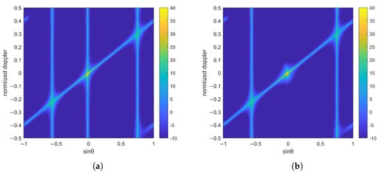
Figure 5.
The estimated capon spectrum of non-target components in Scenario A with the Doppler axis normalized according to the system PRF and the azimuth axis mapped to the sine domain. (a) Before mainlobe jamming separation. (b) After mainlobe jamming separation.
All receivers used the estimated covariance matrix after mainlobe jamming separation to calculate the beamforming matrix for the normal direction. The range of target angle between y-axis was [−5 deg, 5 deg] and the speed of target was [−50 m/s, 50 m/s]. The target velocity vector always pointed to the origin. A total of 1000 Monte Carlo simulations were performed for targets with different directions and speeds, and the average SNR loss after inter-node mainlobe jamming suppression is shown in Figure 6.
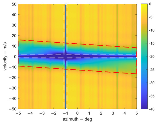
Figure 6.
The average SNR loss of targets at different azimuths (x-axis) and radical velocities (y-axis) after inter-node mainlobe jamming suppression in Scenario A. The suppression area for the actual jamming and clutter is marked with the white dotted line and the extra loss caused by imprecise prior clutter subspace is marked with the red dotted line.
It can be found that the sparse aperture forms a narrow null at the mainlobe jamming direction, which effectively improves the overall SNR with the help of intra-node clutter suppression. Since all nodes only create one beam, the target has a more significant SNR loss at the beam edge than at the beam center. On the other hand, due to the high sidelobe level of the distributed beam pattern, when the target direction is located at a high sidelobe, that is, the correlation coefficient between the steering vector of the target and mainlobe jammer is high, the SNR loss of the target is higher than that of the other directions.
In order to further evaluate the effect of the proposed scheme, the optimal SNR loss of the proposed scheme with an accurate covariance matrix was simulated and compared with the Monte Carlo result in Figure 7.
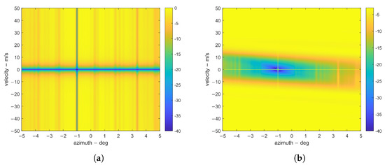
Figure 7.
Comparison between the Monte Carlo results and the theoretical upper bound for target signal-to-noise loss at different azimuths (x-axis) and radial velocities (y-axis) in Scenario A. (a) The ideal SNR loss. (b) The extra SNR loss.
As shown above, when the radial speed of the target exceeds 20 m/s, the additional loss caused by the imprecise covariance matrix is not spatially dependent, and its value is around 4 dB. On the other hand, due to the broadening of the clutter spectrum caused by the residual mainlobe jamming, the proposed scheme has high SNR loss in the low-speed region. Since the spectrum of clutter and jamming intersect obliquely, the outline of the low-SNR region is not parallel to the zero velocity line. The minimum detectable speed of the proposed scheme highly depends on the accuracy of the prior clutter subspace.
In order to demonstrate the increment in mainlobe jamming rejection introduced by the distributed configuration, the SNR loss with only intra-node suppression was only simulated, where the step of mainlobe jamming separation was skipped. The result and comparison are shown in Figure 8. The limited angular resolution of a single antenna array can be verified by the severely widened null along the Doppler domain. The SNR improvement is significant for targets close to the jamming direction.
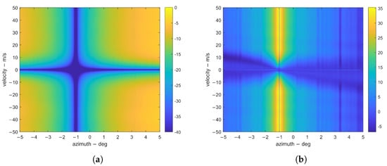
Figure 8.
Comparison of target SNR losses with and without joint processing at different azimuths (x-axis) and radial velocities (y-axis) in Scenario A. (a) The SNR loss. (b) The SNR gain from joint processing.
In order to better demonstrate the improvement in the proposed scheme in the case of insufficient training samples, the traditional joint-domain localization (JDL) algorithm [38] was extended to airborne distributed scenarios for performance comparison. During the JDL processing, each distributed node formed nine space–time beams around the target, and the dimension-reduced data were then directly used for covariance estimation and joint suppression. The output performance of JDL using a different number of training samples was simulated, and the SNR loss of different radial velocity targets at 0 azimuths are compared in Figure 9. As can be found, although JDL reduces the dimension of each node by an order of magnitude, multi-node observation still brings about a significant deterioration when performing inter-node adaptive suppression. When the number of training samples is less than 30, the SNR loss of the extended JDL is more than 10 dB compared with the proposed scheme. Even with 60 training samples, the proposed scheme can still improve the output SNR by approximately 3 dB, whereas the extended JDL obtains better SNR for targets with a radial speed of less than 14 m/s. This result reflects the advantages of the proposed scheme compared with traditional dimension reduction processing.
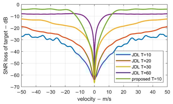
Figure 9.
Comparison of SNR losses of zero-azimuth targets with different radial velocities (x-axis) after suppression with the proposed scheme and the extended JDL in Scenario A.
4.2. Scenario B
The initial coordinates of the distributed node in Scenario B are the same as in Scenario A, and the array antenna of each distributed node is still parallel to the x-axis. However, the nodes fly at different speeds, whose velocity vectors are listed in Table 2.
Table 2.
Velocity vectors of distributed node in Scenario B.
The jammers in sidelobe in Scenario A are kept in Scenario B. The number of instances of mainlobe jamming is increased to 2, and their angle between the y-axis is adjusted to 2 deg and deg. The INR of each jamming signal is still 30 dB. Since Scenario B contains two instances of mainlobe jamming, norm reweighting was performed during mainlobe jamming separation.
Similar to Scenario A, Figure 10 shows the capon spectrum of the first node’s training data before and after mainlobe jamming separation. Since the velocity of each radar node is no longer parallel to the array, the clutter spectrum has apparent curvature in the space Doppler plain. Compared with Figure 5, it can be found that the two instances of mainlobe jamming have evident interaction, and their spectrum also has a curvature along the Doppler axis.
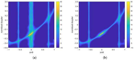
Figure 10.
The estimated capon spectrum of non-target components in Scenario B with the Doppler axis normalized according to the system PRF and the direction axis mapped to the sine domain. (a) Before mainlobe jamming separation. (b) After mainlobe jamming separation.
The SNR loss of targets with the same parameters as Scenario A is simulated in Figure 11, where two narrow lines with high suppression coefficient can be found in the directions of mainlobe jamming. This reflects that the distributed radar forms a synthesized beam with two narrow nulls in this case to reject the jamming energy. Since there is more than one interference source, and the time-varying geometry changes the location of the high sidelobe in distributed beam pattern, the angle with low SNR has a different distribution around the jamming direction compared with Scenario A.
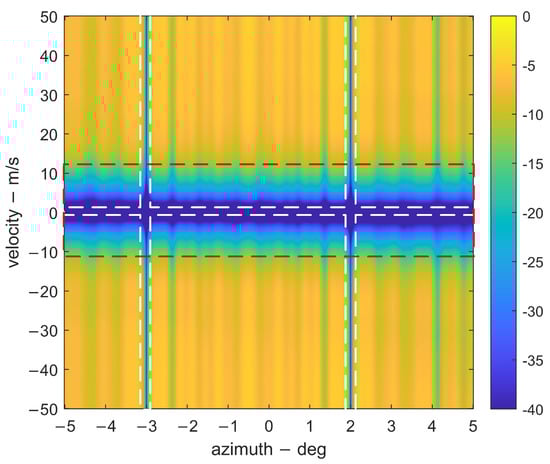
Figure 11.
The average SNR loss of targets at different azimuths (x-axis) and radical velocities (y-axis) after inter-node mainlobe jamming suppression in Scenario B. The suppression area for the actual jamming and clutter is marked with the white dotted line and the extra loss caused by imprecise prior clutter subspace is marked with the red dotted line.
The optimal SNR loss of the proposed scheme with an accurate covariance matrix was simulated and compared with the Monte Carlo result in Figure 12 to further evaluate the proposed scheme’s effect. As can be seen, the additional SNR loss is stable at around 5 dB for targets whose radial speed exceeds 20 m/s. The regression compared with Scenario A can be explained by the jamming energy loss coming from the zero forcing filter in (44) as the correlation coefficient of the steering vector between two instances of mainlobe jamming is much higher. In addition, limited by the angular resolution of the array antenna, the direction of two instances of close mainlobe jamming might be biased. Similar to Scenario A, the Doppler null broadening in Scenario B is also obliquely distributed, but the degree of inclination is reduced due to the smaller slope of the clutter spectrum at the cross point with the jamming spectrum.
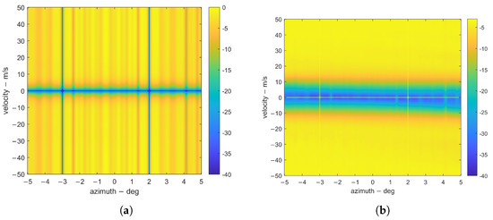
Figure 12.
Comparison between the Monte Carlo results and the theoretical upper bound for target signal-to-noise loss at different azimuths (x-axis) and radial velocities (y-axis) in Scenario B. (a) The ideal SNR loss. (b) The extra SNR loss.
The SNR gain compared with non-joint suppression is also simulated in Figure 13. As shown on the left, a continuous low SNR region in the direction appears between the two instances of mainlobe jamming in the non-joint suppression result. Inter-node suppression can offer approximately 19 dB SNR gain in this area, reflecting the proposed scheme’s adaptability to multiple instances of mainlobe jamming and time-varying distributed aperture.
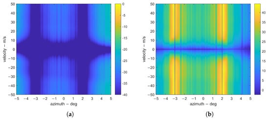
Figure 13.
Comparison of target SNR losses with and without joint processing at different azimuths (x-axis) and radial velocities (y-axis) in Scenario B. (a) The SNR loss without joint processing. (b) The SNR gain from joint processing.
The extended JDL was also simulated for Scenario B and the SNR loss comparison is shown in Figure 14. Due to the increased rank introduced by the added mainlobe jamming, the JDL processing performance under small samples further deteriorated, whereas the other properties are consistent with Scenario A.
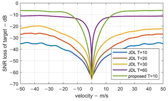
Figure 14.
Comparison of SNR losses of zero-azimuth targets with different radial velocities (x-axis) after suppression with the proposed scheme and the extended JDL in Scenario B.
5. Discussion
The above two numerical examples show the suppression ability of jamming and clutter for distributed radar with the proposed scheme. In this section, several factors affecting the cancellation result are discussed further.
5.1. Inter-Node Narrow Band Assumption
The proposed scheme was derived under the inter-node narrow band assumption. To meet such an assumption, the number of divided sub-bands is extremely large, as the envelope inconsistency of the sidelobe signal in distributed radar is significantly amplified by the sparse observation geometry.
However, during the practical processing, the number of sub-bands should be limited to avoid the extra computational cost and influence of the reduced range resolution. As shown in Figure 3, the suppression of non-target components is split into two stages. In the first stage, each node independently performs mainlobe interference separation and clutter covariance estimation, and clutter is eliminated by intra-node processing. Since there is no joint cancellation, the inter-node decorrelation of clutter will not affect the suppression effect of stage one, which means that the required consistency of the clutter envelope is the same as that of the monostatic airborne radar. As long as the transmitted signal’s bandwidth is narrow for a single antenna array, each distributed node can perform as a monostatic airborne radar and achieve the expected clutter suppression with the proposed scheme.
As for the second stage, joint cancellation is critical to mainlobe jamming because of the significant increment in angular resolution. Although the prior structure is used to estimate , the derivation would not be influenced as the envelope migration would aggravate the inter-node decoherence of clutter, and the block-diagonal structure of is preserved. Only the mainlobe jamming and target echo need to meet the narrow-band assumption of distributed aperture to ensure that coherent processing can accumulate target energy while canceling the jamming component.
Based on the above analysis, the narrow band assumption of the proposed scheme could be relaxed for signals in sidelobes. When the range of the signal’s direction is limited within the mainlobe of a single array antenna, the intrinsic delay difference can be compensated for before the joint process to reduce the range of inter-node envelope migration. This compensation, combined with the reduced direction range of the signal, increases the maximum bandwidth that the scheme can process, which avoids the reduction in training samples caused by excessive sub-band decomposition.
5.2. Influence from Imprecise Prior Clutter Subspace
Before the intra-node clutter cancellation, the proposed scheme first performs mainlobe jamming separation with the projection of a prior clutter subspace. Since the jamming reconstruction is based on its spatial sparsity, the prior subspace must contain the real clutter subspace, and any uncertainty of the clutter ridge obtained from the geometry information would enlarge the minimum spread range of the prior clutter spectrum.
As analyzed above, (25) and (30) cannot reconstruct the jamming component within the prior clutter subspace. The residue mainlobe jamming would be treated as clutter and canceled by each node in the first stage. As a result, the echo of the slow target near the jammed azimuth would be suppressed simultaneously if its Doppler frequency is also located in the prior clutter spectrum’s spread range, leading to the extra loss region in Figure 6 and Figure 11. Since the distribution of clutter ridges is affected by many geometry parameters, it is recommended to calculate its uncertainty using the analytical model directly to obtain the proper tapper factor in (33).
5.3. Covariance Accuracy after Clutter Suppression
Unlike traditional adaptive processing, the inter-node stage in the proposed scheme obtains the covariance estimation based on the jamming mixture model. The unmixed jamming covariance estimation based on a spatial filter is defined in (48), which retains most of the clutter component. Therefore, the accuracy of is mainly determined by the jamming sampling in the weak clutter region. On the other hand, the spatial separation of jamming components from different azimuths also faces the beam distortion problem in traditional adaptive processing. The peak shift of the isolated beam further raises the output noise floor, which, in turn, degrades the estimation performance. Therefore, the processing scheme proposed in this paper will suffer from performance degradation when suppressing multi-mainlobe jamming. Such a phenomenon has been verified by the two numerical examples.
6. Conclusions
In this paper, the jamming and clutter suppression of airborne distributed radar were addressed separately based on their decoherence characteristics. The optimal clutter suppression was achieved at the single-node level, and the subsequent beamforming reduced the data dimension needed for inter-node mainlobe jamming cancellation. Numerical examples demonstrated the effectiveness of the proposed scheme on target SNR improvement and its adaptability to different kinds of distributed geometry. At present, the retention of low-speed targets near the mainlobe jamming is mainly determined by the accuracy of a prior clutter subspace. Possible future works include the accuracy improvement of a clutter subspace based on training data.
Author Contributions
Conceptualization, Y.M. and F.L.; methodology, Y.M. and F.L.; software, Y.M.; formal analysis, Y.M. and F.L.; writing—original draft preparation, Y.M.; visualization, H.L. (Hao Li); writing—review and editing, F.L. and H.L. (Hongjie Liu); project administration, F.L. All authors have read and agreed to the published version of the manuscript.
Funding
This work was supported by the National Key R&D Program of China (grant No. 2021YFB3901400) and the National Natural Science Foundation of China (grant No. 62071045 and grant No. 61625103).
Data Availability Statement
The data that support the findings of this study are available from the corresponding author, F.L., upon reasonable request.
Acknowledgments
The authors thank the editors and anonymous reviewers for their help comments and suggestions.
Conflicts of Interest
The authors declare no conflict of interest.
References
- Ahlgren, G. Next Generation Radar Concept Definition Team Final Report; MIT Lincoln Laboratory: Lexington, MA, USA, 2003. [Google Scholar]
- Cuomo, K.; Coutts, S.; McHarg, J.; Pulsone, N.; Robey, F. Wideband Aperture Coherence Processing for Next Generation Radar (NexGen); Technical Report; Massachusetts Inst of Tech Lexington Lincoln Lab: Lexington, MA, USA, 2004. [Google Scholar]
- Coutts, S.; Cuomo, K.; McHarg, J.; Robey, F.; Weikle, D. Distributed coherent aperture measurements for next generation BMD radar. In Proceedings of the Fourth IEEE Workshop on Sensor Array and Multichannel Processing, Waltham, MA, USA, 12–14 July 2006; pp. 390–393. [Google Scholar]
- Skolnik, M.I. Introduction to Radar Systems; McGraw-Hill Education: New York, NY, USA, 1980. [Google Scholar]
- Yang, Y.; Blum, R.S. Phase synchronization for coherent MIMO radar: Algorithms and their analysis. IEEE Trans. Signal Process. 2011, 59, 5538–5557. [Google Scholar] [CrossRef]
- Yang, X.; Yin, P.; Zeng, T. Time and phase synchronization for wideband distributed coherent aperture radar. In Proceedings of the IET International Radar Conference 2013, Xi’an, China, 14–16 April 2013. [Google Scholar]
- Wang, W.Q. Carrier Frequency Synchronization in Distributed Wireless Sensor Networks. IEEE Syst. J. 2015, 9, 703–713. [Google Scholar] [CrossRef]
- Wang, W.Q. Phase noise suppression in GPS-disciplined frequency synchronization systems. Fluct. Noise Lett. 2011, 10, 303–313. [Google Scholar] [CrossRef]
- Yang, Y.; Blum, R.S. Broadcast consensus based phase synchronization for coherent MIMO radar. In Proceedings of the 2011 45th Annual Conference on Information Sciences and Systems, Baltimore, MD, USA, 23–25 March 2011; pp. 1–6. [Google Scholar] [CrossRef]
- Nanzer, J.A.; Schmid, R.L.; Comberiate, T.M.; Hodkin, J.E. Open-loop coherent distributed arrays. IEEE Trans. Microw. Theory Tech. 2017, 65, 1662–1672. [Google Scholar] [CrossRef]
- Mghabghab, S.R.; Nanzer, J.A. Open-loop distributed beamforming using wireless frequency synchronization. IEEE Trans. Microw. Theory Tech. 2020, 69, 896–905. [Google Scholar] [CrossRef]
- Ellison, S.M.; Mghabghab, S.; Doroshewitz, J.J.; Nanzer, J.A. Combined Wireless Ranging and Frequency Transfer for Internode Coordination in Open-Loop Coherent Distributed Antenna Arrays. IEEE Trans. Microw. Theory Tech. 2020, 68, 277–287. [Google Scholar] [CrossRef]
- Li, Y.; Yang, X.; Liu, F. Robust Adaptive Beamforming for Distributed Radar Based on Covariance Matrix Reconstruction and Steering Vector Estimation. In Proceedings of the 2019 IEEE International Conference on Signal, Information and Data Processing (ICSIDP), Chongqing, China, 11–13 December 2019; pp. 1–4. [Google Scholar]
- Liu, X.; Wang, T.; Chen, J.; Wu, J. Efficient configuration calibration in airborne distributed radar systems. IEEE Trans. Aerosp. Electron. Syst. 2022, 58, 1799–1817. [Google Scholar] [CrossRef]
- Liu, X.; Wang, T.; Chen, J.; Wu, J. Efficient configuration calibration using ground auxiliary receivers at inaccurate locations. Digit. Signal Process. 2022, 129, 103675. [Google Scholar] [CrossRef]
- Lu, J.; Liu, F.; Sun, J.; Miao, Y.; Liu, Q. Distributed Radar Robust Location Error Calibration Based on Interplatform Ranging Information. In Proceedings of the 2019 IEEE International Conference on Signal, Information and Data Processing (ICSIDP), Chongqing, China, 11–13 December 2019; pp. 1–5. [Google Scholar] [CrossRef]
- Sun, P.; Tang, J.; Tang, X. Cramer-Rao bound and signal-to-noise ratio gain in distributed coherent aperture radar. J. Syst. Eng. Electron. 2014, 25, 217–225. [Google Scholar] [CrossRef]
- Chen, J.; Wang, T.; Liu, X.; Wu, J. Identifiability Analysis of Positioning and Synchronization Errors in Airborne Distributed Coherence Aperture Radars. IEEE Sens. J. 2022, 22, 5978–5993. [Google Scholar] [CrossRef]
- Lu, J.; Liu, F.; Liu, H.; Liu, Q. Target Localization Based on High Resolution Mode of MIMO Radar with Widely Separated Antennas. Remote Sens. 2022, 14, 902. [Google Scholar] [CrossRef]
- Vukmirović, N.; Erić, M.; Janjić, M.; Djurić, P.M. Direct wideband coherent localization by distributed antenna arrays. Sensors 2019, 19, 4582. [Google Scholar] [CrossRef] [PubMed]
- Long, T.; Zhang, H.; Zeng, T.; Liu, Q.; Chen, X.; Zheng, L. High accuracy unambiguous angle estimation using multi-scale combination in distributed coherent aperture radar. IET Radar Sonar Navig. 2017, 11, 1090–1098. [Google Scholar] [CrossRef]
- Liu, Y. Structure-based joint estimation algorithm for distributed coherent aperture radar. J. Eng. 2020, 2020, 1123–1130. [Google Scholar] [CrossRef]
- Yin, P.; Yin, W.; Li, H.; Liang, Z.; Liu, Z.; Liu, Q. Estimation method of coherent efficiency of distributed coherent aperture radar based on cross-correlation. In Proceedings of the ET International Radar Conference 2015, Hangzhou, China, 14–16 October 2015. [Google Scholar]
- Chen, J.; Chen, X.; Zhang, H.; Zhang, K.; Liu, Q. Suppression Method for Main-Lobe Interrupted Sampling Repeater Jamming in Distributed Radar. IEEE Access 2020, 8, 139255–139265. [Google Scholar] [CrossRef]
- Ge, M.; Cui, G.; Kong, L. Mainlobe jamming suppression for distributed radar via joint blind source separation. IET Radar Sonar Navig. 2019, 13, 1189–1199. [Google Scholar] [CrossRef]
- Chen, X.; Shu, T.; Yu, K.B.; He, J.; Yu, W. Joint Adaptive Beamforming Techniques for Distributed Array Radars in Multiple Mainlobe and Sidelobe Jammings. IEEE Antennas Wirel. Propag. Lett. 2020, 19, 248–252. [Google Scholar] [CrossRef]
- Zhang, Q.; Gao, F.; Sun, Q.; Wang, X. Mainlobe jamming cancelation method for distributed monopulse arrays. Sci. China Inf. Sci. 2018, 61, 1–3. [Google Scholar] [CrossRef]
- Zeng, T.; Yin, P.; Liu, Q. Wideband distributed coherent aperture radar based on stepped frequency signal: Theory and experimental results. IET Radar Sonar Navig. 2016, 10, 672–688. [Google Scholar] [CrossRef]
- Brookner, E. Adaptive Antennas, Concepts and Performance. IEEE Antennas Propag. Soc. Newsl. 1988, 30, 37. [Google Scholar] [CrossRef]
- Petraglia, M.; Mitra, S. Performance analysis of adaptive filter structures based on subband decomposition. In Proceedings of the 1993 IEEE International Symposium on Circuits and Systems, Chicago, IL, USA, 3–6 May 1993; Volume 1, pp. 60–63. [Google Scholar] [CrossRef]
- Liu, W.; Langley, R.J. An Adaptive Wideband Beamforming Structure with Combined Subband Decomposition. IEEE Trans. Antennas Propag. 2009, 57, 2204–2207. [Google Scholar] [CrossRef]
- Goodman, N.A.; Stiles, J.M. On clutter rank observed by arbitrary arrays. IEEE Trans. Signal Process. 2006, 55, 178–186. [Google Scholar] [CrossRef]
- Tang, G.; Bhaskar, B.N.; Shah, P.; Recht, B. Compressed sensing off the grid. IEEE Trans. Inf. Theory 2013, 59, 7465–7490. [Google Scholar] [CrossRef]
- Yang, Z.; Xie, L. Enhancing sparsity and resolution via reweighted atomic norm minimization. IEEE Trans. Signal Process. 2015, 64, 995–1006. [Google Scholar] [CrossRef]
- Dunning, I.; Huchette, J.; Lubin, M. JuMP: A Modeling Language for Mathematical Optimization. SIAM Rev. 2017, 59, 295–320. [Google Scholar] [CrossRef]
- Garstka, M.; Cannon, M.; Goulart, P. COSMO: A Conic Operator Splitting Method for Convex Conic Problems. J. Optim. Theory Appl. 2021, 190, 779–810. [Google Scholar] [CrossRef]
- Zheng, Y.; Fantuzzi, G.; Papachristodoulou, A.; Goulart, P.; Wynn, A. Fast ADMM for semidefinite programs with chordal sparsity. In Proceedings of the 2017 American Control Conference (ACC), Seattle, WA, USA, 24–26 May 2017; pp. 3335–3340. [Google Scholar]
- Wang, H.; Cai, L. On adaptive spatial-temporal processing for airborne surveillance radar systems. IEEE Trans. Aerosp. Electron. Syst. 1994, 30, 660–670. [Google Scholar] [CrossRef]
Publisher’s Note: MDPI stays neutral with regard to jurisdictional claims in published maps and institutional affiliations. |
© 2022 by the authors. Licensee MDPI, Basel, Switzerland. This article is an open access article distributed under the terms and conditions of the Creative Commons Attribution (CC BY) license (https://creativecommons.org/licenses/by/4.0/).