Article

Intersection Constraint Weighting (ICW) Method: High-Resolution Joint Magnetic Susceptibility Inversion of Aeromagnetic and Gradient Data

1
College of Geoexploration Science and Technology, Jilin University, Changchun 130026, China
2
Laboratory of Science and Technology on Marine Navigation and Control, China State Shipbuilding Corporation, Tianjin 300131, China
*
Author to whom correspondence should be addressed.
Remote Sens. 2022, 14(23), 6029; https://doi.org/10.3390/rs14236029
Submission received: 3 November 2022 / Revised: 18 November 2022 / Accepted: 25 November 2022 / Published: 28 November 2022
(This article belongs to the Section Earth Observation Data)

Abstract

:
Aeromagnetic gradient data have higher horizontal resolution on shallow sources, a magnetic anomaly that can better reflect the features of deeper sources. Therefore, we used a joint survey of aeromagnetic and gradient data to obtain the distribution of sources with different depths. In this paper, we propose an intersection constraint weighting (ICW) method based on aeromagnetic and gradient data for original and gradient anomalies with inconsistent high-low variation characteristics. The ICW method can effectively improve the resolution of inversion results and can more accurately obtain the distribution of magnetic bodies via cross-gradient by gradually adding a gradient component and applying a normalized property weighting function. Our theoretical model tests indicate that the distribution of the recovered magnetic susceptibility model of the ICW method was similar to that of the true model. In addition, the anomaly containing noise with different signal-to-noise ratios verified that the ICW method had a stronger anti-noise ability than other methods. We also inverted real data in the Zhurihe area of the Inner Mongolia Autonomous Region in northern China. The inversion result showed that the main trend of high magnetic bodies was in the northeast direction, that the shallowest depth of high magnetic bodies was 100 m, and that the greatest depth was 960 m.

Graphical Abstract

1. Introduction

Metal mineral resources generally have high magnetic susceptibility, so they appear as high-value anomalies in magnetic exploration. Aeromagnetic surveys are unrestricted by terrain, fast and economical, and widely employed in practice [1,2]. The magnetic susceptibility inversion results of magnetic anomalies can be used to delineate the distribution of magnetic ore bodies [2,3,4,5,6,7,8]. Bott [9] applied the matrix linear solution to determine the magnetic susceptibility distribution. Arkani-Hamed and Stranqway [10] developed a technique to invert a scalar magnetic anomaly map into a magnetic susceptibility anomaly map. Well-defined susceptibility highs are associated with the Kursk iron formation and small-scale shields and plates, and well-defined susceptibility lows delineate collision zones in the Alpine-Himalayan belt. Li and Oldenburg [11] elaborated the regularization solution method of 3D physical property inversion of magnetic data and obtained a 3D magnetic susceptibility distribution by introducing model constraints and a depth-weighting function. Pilkington [12] presented a preconditioned conjugate gradient approach to solve the 3D magnetic inversion problem with the least amount of prior information to determine the magnetic susceptibility distribution of a given magnetic anomaly. Li and Oldenburg [13] developed a fast inversion method based on wavelet compression and a logarithmic barrier of minimization to recover the 3D distribution of magnetic susceptibility. Pilkington [14] introduced the 3D sparse inversion of aeromagnetic data combined with the conjugate gradient algorithm to improve the resolution of the inversion results. Li et al. [15] developed a level-set approach to determine the magnetic susceptibility value through joint inversion of surface and borehole magnetic data, which can be utilized as a probing parameter to assess the uncertainty in the spatial extent of causative bodies.
Different gravity gradient tensor components can enhance different characteristics of the field source [16]. Different components have different resolutions for the source, and due to the lack of a calculation method, different components will produce different inversion results [17,18,19]. Certain scholars have improved the effect of model reconstruction by adding anomaly components during inversion [20,21]. Qin et al. [22] directly integrated different gravity gradient components into a matrix to improve the resolution of inversion results. Magnetic gradient data have a higher horizontal resolution than magnetic anomalies, effectively highlighting shallow geological bodies, while original magnetic data can more effectively retain deep field source information. Therefore, the joint exploration of aeromagnetic fields and their gradients is commonly performed to delineate metal mineral resources [23,24,25,26,27,28].
The conventional joint inversion method is data joint inversion. which superimposes the original magnetic anomaly onto the magnetic gradient anomaly in a matrix to improve the precision of inversion results using weight constraints of different anomaly components [29]. Joint inversion based on structural constraints is another way to improve inversion resolution, such as the cross-gradient method, which is mostly utilized for the inversion of different types of data [30,31,32,33,34,35,36]. The structure factor of the cross-gradient has a better constraining effect on the magnetic and magnetic gradient data of the same source and different resolutions, which can improve the inversion precision and satisfy the consistency of the magnetic and magnetic gradient inversion results of the final results of the ICW method.
To improve the resolution and precision of the joint inversion of aeromagnetic and gradient data and to better reveal the distribution of the magnetic sources, this paper proposes an intersection constraint weighting (ICW) method. The ICW method involves a data constraint strategy, model weighting function design, and a step-by-step, cross-gradient constraint calculation process to obtain higher resolution inversion results. The precision and practicability of the method are proven by theoretical model tests and real data application.

2. Methodology

2.1. Data Joint Inversion

Magnetic susceptibility inversion divides the underground into grids according to the measurement point distance, calculates the magnetic susceptibility of each grid, and then obtains the distribution of the underground field source. The number of divided grids generally exceeds the number of observation points. There are two main ways to realize the joint magnetic susceptibility inversion of aeromagnetic and gradient data. A more commonly employed inversion method is putting different parameter data in a matrix to achieve magnetic susceptibility constrained inversion, which is named data joint inversion [29]. The objective function is
Φ D J = W d D J G Δ T G Δ T x G Δ T y G Δ T z m 2 d Δ T d Δ T x d Δ T y d Δ T z 2 2 + δ W m D J m 2 2 2 min ,
where d Δ T is the magnetic anomaly and d Δ T x , d Δ T y , and d Δ T z are the magnetic gradients in the x -direction, y -direction, and z -direction, respectively. The matrices G Δ T , G Δ T x , G Δ T y , and G Δ T z are the forward operators that connect the observation data with the physical parameter [12]. The column vector m 2 represents the physical parameter (magnetic susceptibility) inverted by the combined matrix d Δ T ; d Δ T x ; d Δ T y ; d Δ T z . δ is the regularization parameter, and we use the L-curve method to determine the regularization parameters [37]. W m D J is the model weighting matrix [38,39], and W d D J is the data weighting matrix [11].

2.2. Cross-Gradient Inversion

cross-gradient inversion is another method that can be utilized for joint magnetic susceptibility inversion of aeromagnetic and gradient data by using the gradient change in physical properties as structural constraints to improve the resolution of inversion results. The objective functions are
Φ Δ T = W d Δ T G Δ T m Δ T d Δ T 2 2 + δ W m Δ T m Δ T 2 2 + γ Φ c g min
Φ Δ T g = W d Δ T g G Δ T x G Δ T y G Δ T z m Δ T g d Δ T x d Δ T y d Δ T z 2 2 + δ W m Δ T g m Δ T g 2 2 + γ Φ c g min
where γ is the coefficient of the cross-gradient term, Φ c g = t x , y , z 2 2 is the cross-gradient term [31], and t x , y , z is calculated by
t x , y , z = m Δ T × m Δ T g = t x , t y , t z ,   where t x m Δ T , m Δ T g = m Δ T g y , z y m Δ T y , z z m Δ T y , z y m Δ T g y , z z t y m Δ T , m Δ T g = m Δ T g x , z x m Δ T x , z z m Δ T x , z x m Δ T g x , z z t z m Δ T , m Δ T g = m Δ T g x , y x m Δ T x , y y m Δ T x , y x m Δ T g x , y y
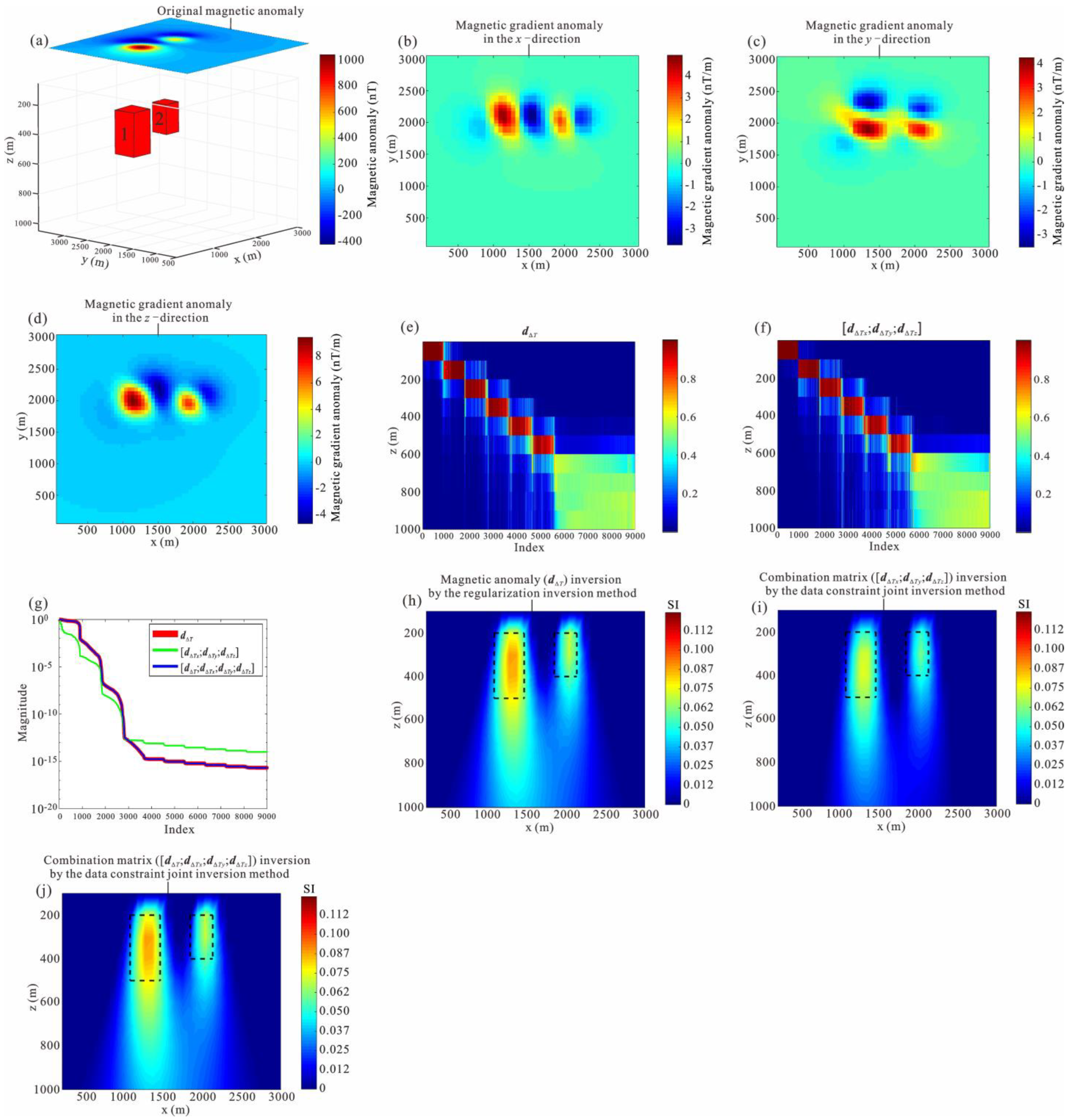
To verify the resolution and depth information of different components of magnetic and gradient data to different depths, we introduce depth resolution plots (DRPs) [40] and eigenvalue spectra for kernel function matrices [16]. The source volume has dimensions of 3 × 3 × 1 km, which is discretized with n x = n y = 30 and n z = 10 ; that is, the solution domain consists of n = 9000 cells. The data grid covers an area of 3 km × 3 km, and they are measured at ground level. For the first case, which uses a combination of magnetic gradients in the x -direction, y -direction, and z -direction, the data points p of each gradient anomaly are arranged in a 30 × 30 grid ( p = 900 ). For the magnetic anomaly component, the data points are arranged in a 54 × 50 grid ( p = 2700 ).
Consider a model that contains two prisms with the same burial depths, where the top burial depth and bottom burial depth of prism 1 and prism 2 are 300 m and 500 m and 300 m and 400 m, respectively, and the real magnetic susceptibility is 0.25. The inclination and declination are 45° and 60°, respectively.
Figure 1a shows a 3D view of the model and the corresponding magnetic anomaly with a flight height of 100 m, and Figure 1b–d shows gradient anomalies in the x -direction, y -direction and z -direction. The dotted line indicates the real position of the geological body.
Figure 1e,f are the DRP of the magnetic and combination matrix of gradient components for the first case. As the depth increases, the depth resolution decreases, and when the depth is shallower, the resolution of the combination matrix of gradient components is relatively high. Figure 1e–g shows the corresponding eigenvalue spectra for the kernel function matrices. In the first 900, the depth information carried by the combination matrix of gradient components is slightly lower than that of the combination matrix of magnetic and gradient components. In the latter 1800, the depth information carried by the combination matrix of gradient components decays more slowly. It can be seen from the inversion results in Figure 1h–j that the resolution of the combination matrix ( d Δ T x ; d Δ T y ; d Δ T z ) inversion is worse and that the magnetic anomaly ( d Δ T ) inversion results are similar to the combined matrix ( d Δ T ; d Δ T x ; d Δ T y ; d Δ T z ) inversion, indicating that the addition of gradient components cannot improve the resolution of the inversion results, which is consistent with the conclusion of Paoletti et al. [16].
For the second case, which uses a combination of magnetic gradients in the x -direction, y -direction, and z -direction, the data points of each gradient anomaly are arranged in a 62 × 50 grid ( p = 3100 ). For the magnetic anomaly component, the data points are arranged in a 100 × 93 grid ( p = 9300 ). In Figure 2e,f, we discovered that the depth resolution of the combination matrix of gradients is higher than that of the magnetic matrix when the depth is shallow, which is consistent with the conclusion of Figure 1. In Figure 1g, the depth information of the combination matrix of gradients decays the slowest, and the decay trend of the depth information of the magnetic component is consistent with the decay trend of the combination matrix of the magnetic and gradient components. The figure also shows that the depth information carried in each singular vector is almost independent of the number p . In Figure 2h–j, the resolution of the combination matrix ( d Δ T x ; d Δ T y ; d Δ T z ) inversion is slightly improved with an increase in the number of data points, and the results of the magnetic anomaly ( d Δ T ) inversion and combination matrix ( d Δ T ; d Δ T x ; d Δ T y ; d Δ T z ) inversion are similar to those shown in Figure 1. In general, the addition of gradient components does not contribute to the improvement in inversion resolution with the same burial depth and similar characteristics of magnetic and gradient anomalies. Next, we will discuss the situation of different burial depths of subsurface geological bodies and different characteristics of magnetic and gradient anomalies.
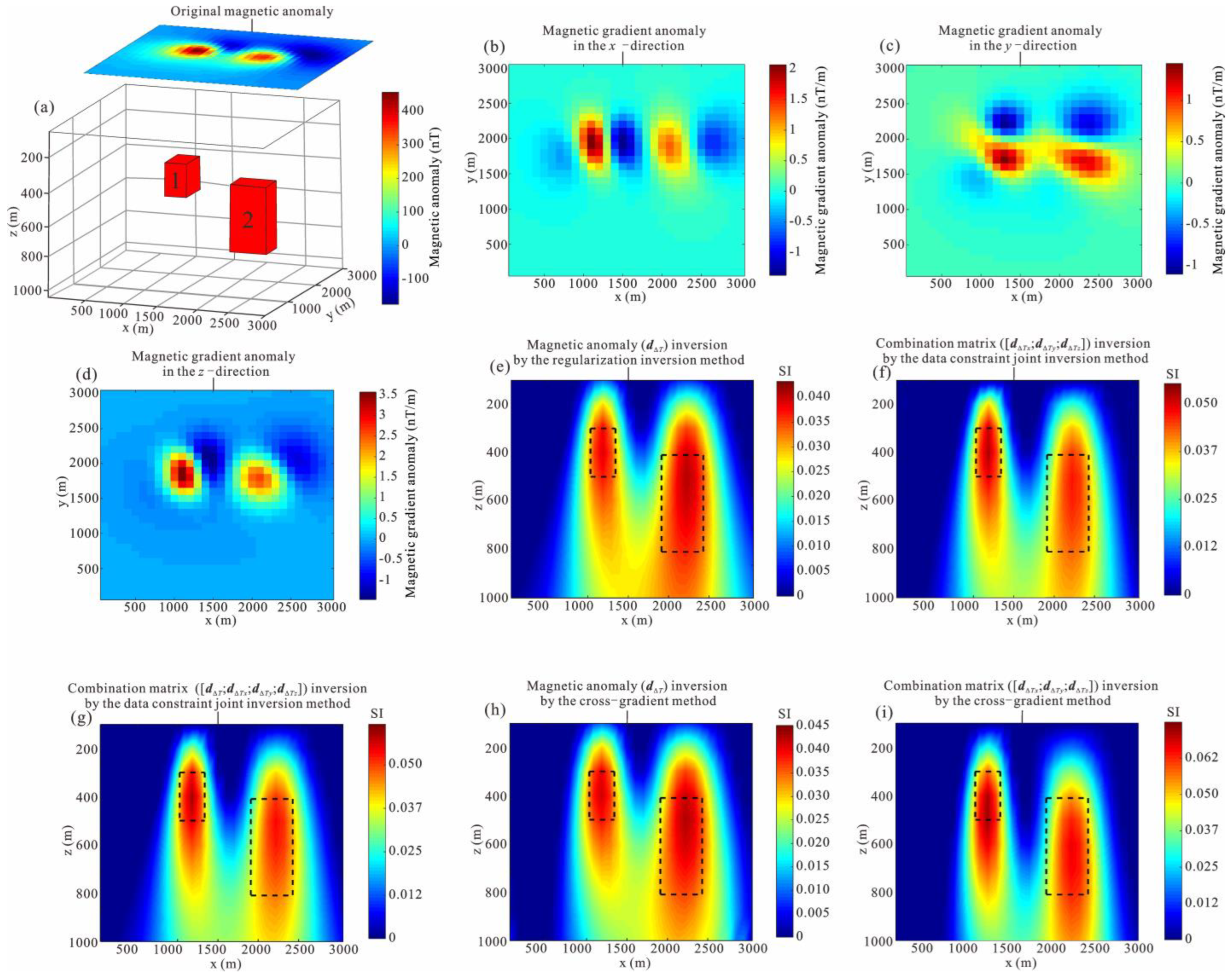
A model that contains two prisms with different burial depths, different sizes, and identical physical properties was designed to test the effect of the existing method. The top burial depth and bottom burial depth of prism 1 and prism 2 were 300 m and 500 m and 400 m and 800 m, respectively, and the real magnetic susceptibility was 0.25. The inclination and declination were 45° and 60°, respectively.
Figure 3a is a 3D view of the model and the corresponding magnetic anomaly with a flight height of 100 m, and Figure 3b–d shows gradient anomalies in the x -direction, y -direction and z -direction. The dotted line indicates the horizontal position of the geological body.
Figure 3e shows a magnetic susceptibility slice ( y = 1900 m) by regularization inversion of the magnetic anomaly. The result can better reflect the distribution of deeper geological bodies, but the resolution is lower. Figure 3f is the magnetic susceptibility slice ( y = 1900 m) obtained by data constraint joint inversion of the combination matrix ( d Δ T x ; d Δ T y ; d Δ T z ). The result better highlights the shallower geological body. It has a higher horizontal resolution, but the deviation between the inversion result of the deep field source and the real model is larger. Compared with Figure 3e,f, the inversion results of the deep geological body with the original anomaly are better than those of the gradient anomaly, while the inversion results of the shallow geological body with the gradient anomaly are better than those of the original anomaly, and the resolution is higher than that of the original anomaly. Figure 3g is the magnetic susceptibility slice ( y = 1900 m) obtained by data constraint joint inversion of the combination matrix ( d Δ T ; d Δ T x ; d Δ T y ; d Δ T z ), which further improves the effect of shallow geological bodies but remains poor for deeper geological bodies. Integrating different components into a matrix for inversion is an effective way to improve the resolution of the inversion results [22].
Figure 3h,i show magnetic susceptibility slices ( y = 1900 m) obtained by cross-gradient inversion of the magnetic anomaly and combination matrix ( d Δ T x ; d Δ T y ; d Δ T z ), respectively. Compared with Figure 3e,f, the horizontal resolution of deep and shallow geological bodies is higher. However, the distinct distribution of geological bodies of different depths still cannot be obtained simultaneously, and the value of magnetic susceptibility is still quite different from the true magnetic susceptibility.

2.3. Intersection Constraint Weighting (ICW) Method

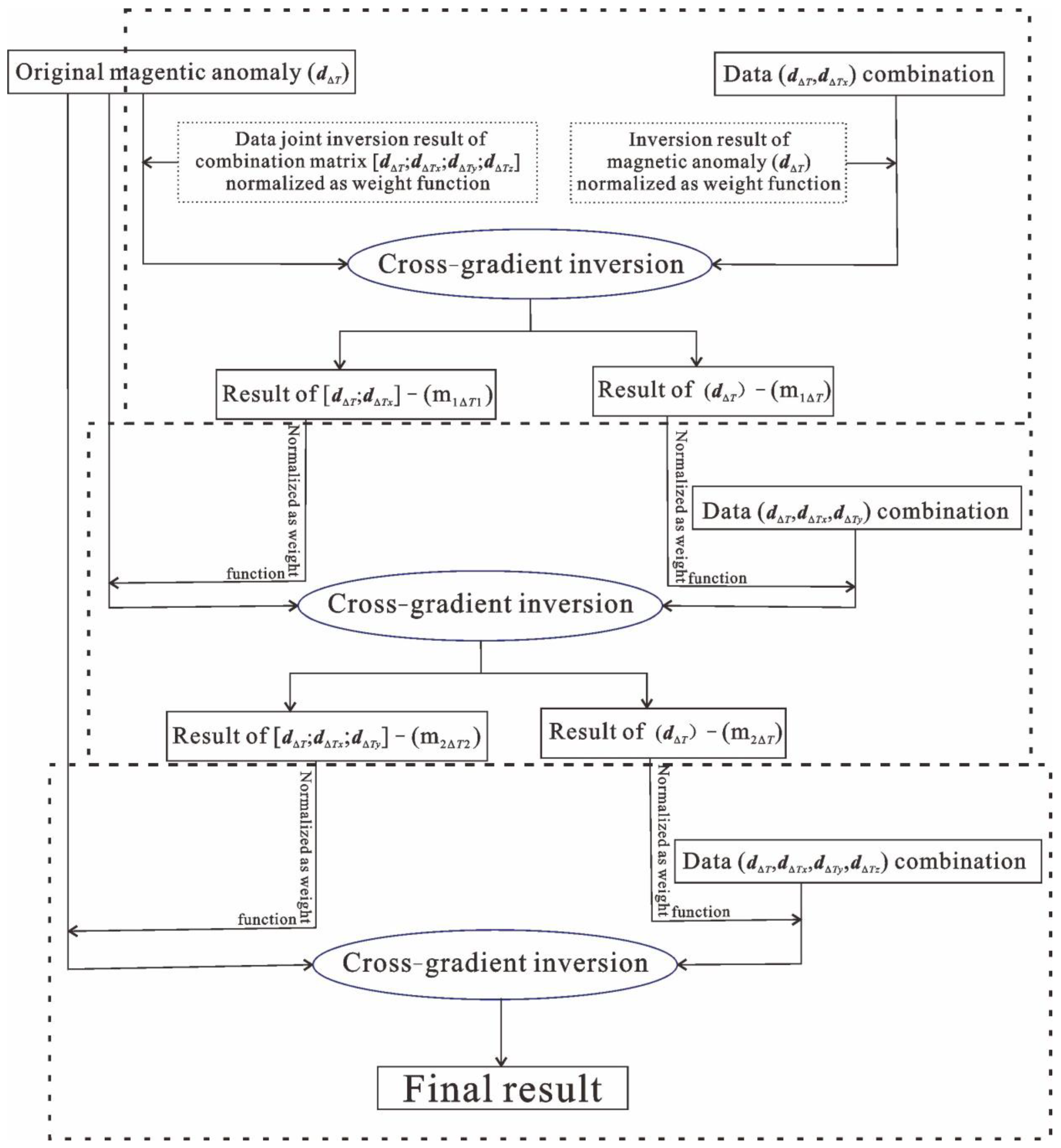
To obtain higher resolution and precision inversion results, we propose an ICW method that gradually adds the gradient data, normalizes the inversion result as a weight function, and uses the cross-gradient to realize the structure constraint. First, the regularization inversion result and data constraint joint inversion result are normalized as the weight function of magnetic anomaly inversion and the combination matrix ( d Δ T ; d Δ T x ) inversion, respectively. The objective functions are
Φ Δ T = W d Δ T G Δ T m 1 Δ T d Δ T 2 2 + δ W m Δ T m 1 Δ T 2 2 + γ Φ c g min
Φ Δ T 1 = W d Δ T 1 G Δ T G Δ T x m 1 Δ T 1 d Δ T d Δ T x 2 2 + δ W m Δ T 1 m 1 Δ T 1 2 2 + γ Φ c g min
where
W m Δ T = i = 1 N G Δ T i j 2 β 4 d i a g m 2 min m 2 max m 2 min m 2 , j = 1 , , M ,   W m Δ T 1 = i = 1 2 N G Δ T 1 i j 2 β 4 d i a g m 1 min m 1 max m 1 min m 1 , j = 1 , , M ,   N
is the number of data, M is the number of cells in the discretized model, and G Δ T 1 = G Δ T G Δ T x . 0.5 < β < 1.5 , the value for β should usually be near 1 [39]. m 1 and m 2 are the magnetic susceptibility results of regularization inversion and data constraint joint inversion, respectively, in (1). Here, the result with a better shallow inversion effect is applied as the weight to highlight the deep anomaly, and the result with a better deep inversion effect is selected as the weight to highlight the shallow anomaly. The cross use of this result weight can improve the resolution of field sources at different depths.
Second, the gradient anomaly in the y -direction is added in the inversion, m 1 Δ T 1 calculated in the previous step is taken as the weight of the magnetic anomaly inversion, and m 1 Δ T is taken as the weight of the combination matrix ( d Δ T ; d Δ T x ; d Δ T y ) inversion. The objective functions are
Φ Δ T = W d Δ T G Δ T m 2 Δ T d Δ T 2 2 + δ W m Δ T m 2 Δ T 2 2 + γ Φ c g min
Φ Δ T 2 = W d Δ T 2 G Δ T G Δ T x G Δ T y m 2 Δ T 2 d Δ T d Δ T x d Δ T y 2 2 + δ W m Δ T 2 m 2 Δ T 2 2 2 + γ Φ c g min
where m 2 Δ T and m 2 Δ T 2 are the magnetic susceptibility inversion results.
The gradient anomaly in the z -direction is added to the inversion, m 2 Δ T 2 calculated in the previous step, is used as the weight of the magnetic anomaly inversion, and m 2 Δ T is used as the weight of the combination matrix ( d Δ T ; d Δ T x ; d Δ T y ; d Δ T z ) inversion. The objective functions are
Φ Δ T 3 = W d Δ T 3 G Δ T G Δ T x G Δ T y G Δ T z m 3 Δ T 3 d Δ T d Δ T x d Δ T y d Δ T z 2 2 + δ W m Δ T 3 m 3 Δ T 3 2 2 + γ Φ c g min
where m 3 Δ T 3 is the final result by the ICW method, which can simultaneously achieve data and structure constraints, effectively balance the field source responses at different depths, and improve the resolution and precision of the inversion result. The specific implementation process is shown in Figure 4.

3. Theoretical Model Tests

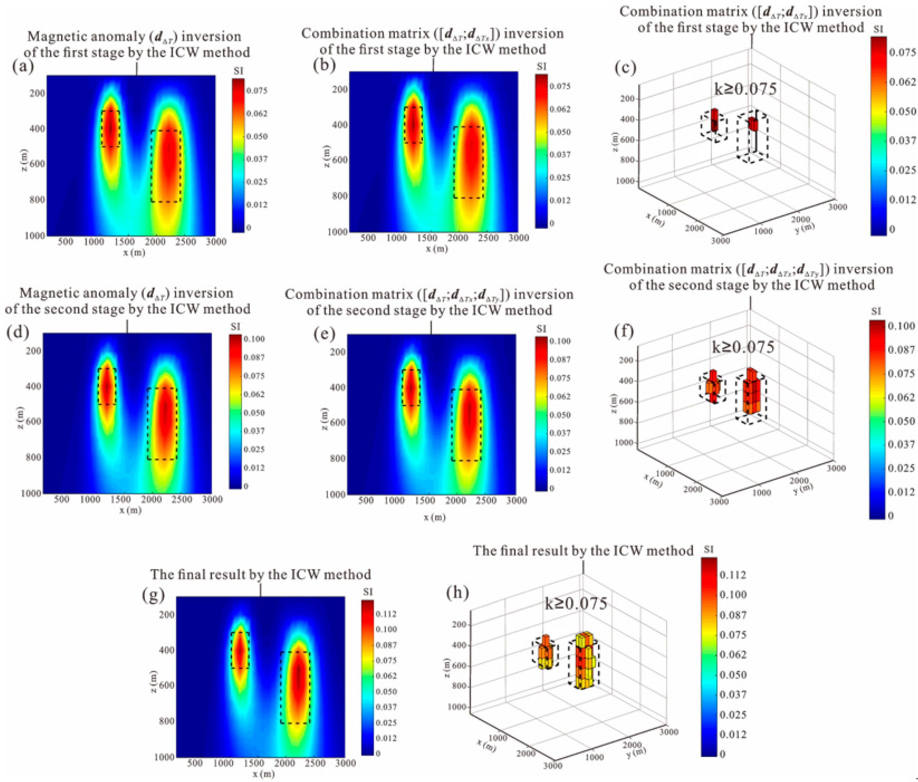
The model shown in Figure 3 was used to verify the effect of the ICW method. To highlight the gradual improvement in the inversion performance at each stage of the method, we set the same truncated magnetic susceptibility. Figure 5a,b show the magnetic susceptibility slices ( y = 1900 m) of the first stage of magnetic anomaly inversion and combination matrix ( [ d Δ T ; d Δ T x ] ) inversion by the ICW method. Figure 5c shows the volume-rendered image of the combination matrix ( [ d Δ T ; d Δ T x ] ) inversion of the first stage by the ICW method with a magnetic susceptibility larger than 0.075. The resolution and precision of the inversion results in Figure 5a,b are significantly better than those of the data constraint joint Inversion and the cross-gradient inversion, but the inversion results in Figure 5c deviate greatly from the real model. Figure 5d,e show the magnetic susceptibility slices ( y = 1900 m) of the second stage of magnetic anomaly inversion and combination matrix ( [ d Δ T ; d Δ T x ; d Δ T y ] ) inversion by the ICW method. Figure 5f shows the volume-rendered image of the combination matrix ( [ d Δ T ; d Δ T x ; d Δ T y ] ) inversion of the second stage by the ICW method with a magnetic susceptibility larger than 0.075. Compared with the inversion results of the first stage, the resolution is further improved, and the value of magnetic susceptibility is somewhat closer to the true magnetic susceptibility; however, there is still a difference with the real location of the model. Figure 5g shows the magnetic susceptibility slice ( y = 1900 m) of the final result by the ICW method. Figure 5h shows the volume-rendered image of the final result by the ICW method with a magnetic susceptibility larger than 0.075. Compared with the inversion results of the second stage, the value of magnetic susceptibility is closer to the true magnetic susceptibility, and the position and shape of the recovered magnetic susceptibility distribution are more consistent with the real model. Variable k represents the truncated magnetic susceptibility. The dotted prism identifies the real model.
The burial depth of the two prisms included in the model in Figure 3 is simultaneously increased by 100 m, and the 3D distribution of the model and the corresponding anomalies are obtained, as shown in Figure 6a–d. The magnitude of the magnetic and gradient anomalies is further reduced, which will greatly affect the resolution and precision of the inversion. Figure 6e shows the volume-rendered images of the data constraint joint inversion of the combination matrix ( [ d Δ T ; d Δ T x ; d Δ T y ; d Δ T z ] ) with a magnetic susceptibility larger than 0.028. When the truncated magnetic susceptibility is similar to the real magnetic susceptibility to the greatest extent, it can recover the deep geological body better but cannot restore the shallow geological body. Figure 6f,g show the volume-rendered images of the magnetic anomaly inversion and combination matrix ( [ d Δ T ; d Δ T x ; d Δ T y ] ) inversion by the cross-gradient method. Compared with Figure 6e, Figure 6f recovers the deep geological body better but still cannot recover the shallow geological body. In Figure 6g, when the truncated magnetic susceptibility is larger, more deep geological bodies can be recovered, and shallow geological bodies can be recovered to a certain extent, but the recovered model is quite different from the real model position (dotted box). Compared with Figure 6e–g, the ICW method recovers the model best, and the value of magnetic susceptibility is closer to the real magnetic susceptibility. However, in general, when the distance between the measurement and the field source is increased, the resolution of the inversion will inevitably be reduced, which will adversely affect the recovery of the model. Compared with other methods, the ICW method still has absolute advantages in this case.
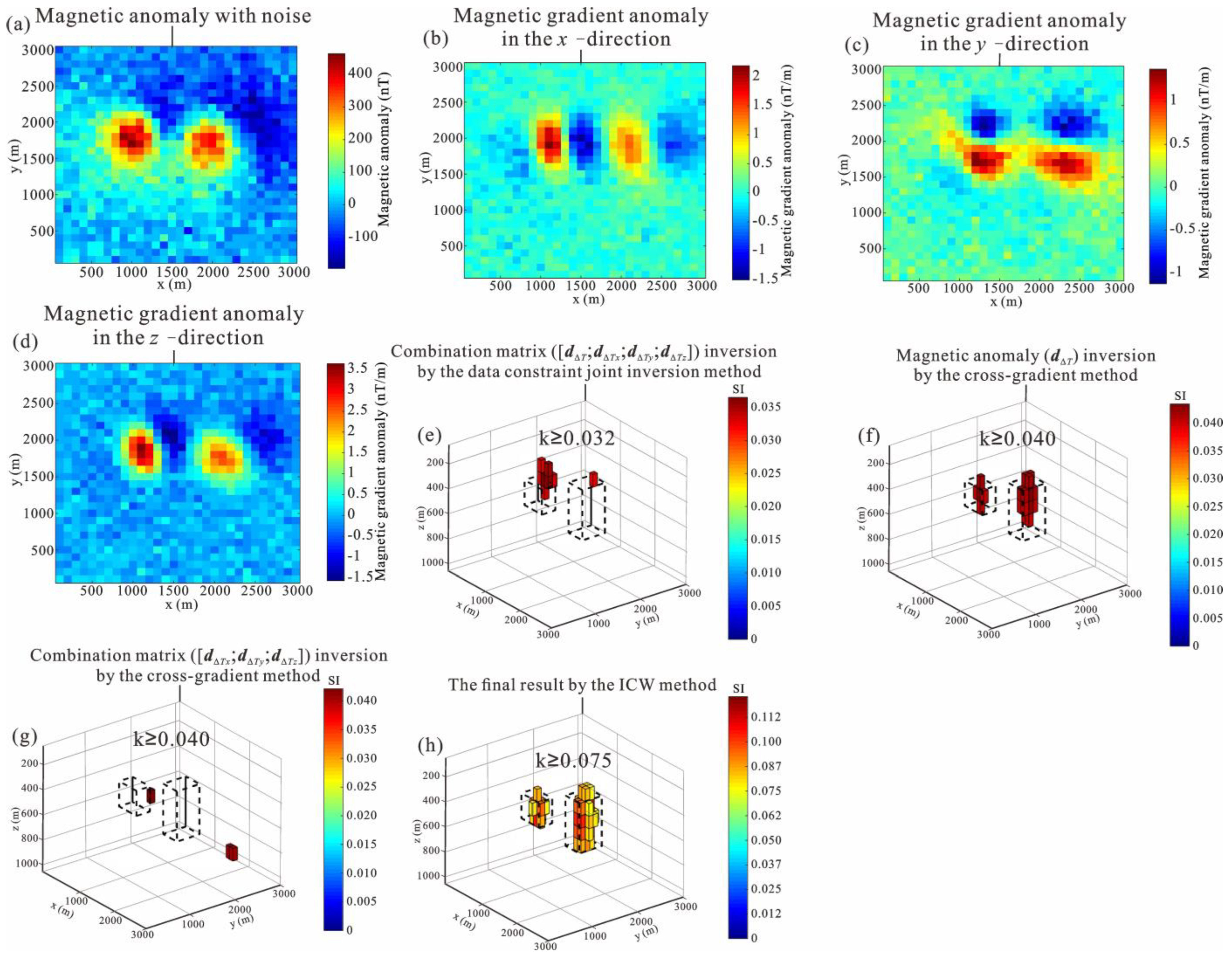
In actual situations, anomalous data will inevitably be disturbed by noise. We add Gaussian noise with a signal-to-noise ratio of 20 to the magnetic and gradient anomalies in Figure 3, as shown in Figure 7a–d.
Figure 7e shows the volume-rendered image of the combination matrix ( [ d Δ T ; d Δ T x ; d Δ T y ; d Δ T z ] ) inversion by the data constraint joint inversion method with a magnetic susceptibility larger than 0.032, which is quite different from the real model. Figure 7f,g show the volume-rendered images obtained by cross-gradient inversion of the magnetic anomaly and combination matrix ( [ d Δ T ; d Δ T x ; d Δ T y ] ), respectively. Figure 7f compares Figure 7e,g with the truncated magnetic susceptibility closer to the real magnetic susceptibility, which restores a better magnetic susceptibility model for deep and shallow geological bodies. Although Figure 7g also restores the magnetic susceptibility model, it completely deviates from the real model position. Figure 7h shows the volume-rendered image of the final result by the ICW method with a magnetic susceptibility larger than 0.075. Compared with the inversion results of the previous methods, the value of magnetic susceptibility obtained by the ICW method is closer to the true magnetic susceptibility ( κ = 0.25 ), and the magnetic susceptibility model recovered when the truncated magnetic susceptibility was most similar to the real model. Compared with the inversion results in Figure 5, the value of magnetic susceptibility is higher and the recovered magnetic susceptibility model is better, indicating that the ICW method has strong noise immunity.
To further verify the sensitivity of the ICW method to noise intensity, we added Gaussian noise with a signal-to-noise ratio of 10 to the magnetic and gradient anomalies in Figure 3, as shown in Figure 8a–d. Using the same truncated magnetic susceptibility as the methods corresponding to Figure 7, the volume-rendered images of Figure 8 were obtained. We discovered that the magnetic susceptibility models recovered by the data constraint joint inversion method and cross-gradient method in Figure 8e–g were worse and that the precision was further reduced. Only the magnetic susceptibility model recovered by the ICW method in Figure 8h is almost the same as that without noise, which further verifies that the ICW method is extremely insensitive to noise.
Considering the complexity of the actual underground situation, we designed a model that contains four anomalous bodies with different burial depths to test the applicability of the ICW method. The top and bottom burial depths of prisms 1 and 3 and prisms 2 and 4 were 200 m and 400 m and 300 m and 700 m, respectively. The magnetic susceptibility was 0.25, and the inclination and deflection were 45° and 60°, respectively. The specific distribution of the model and corresponding magnetic anomaly are shown in Figure 9a.
Figure 9b–d show the magnetic gradient anomalies in the x -direction, y -direction, and z -direction with a flight height of 100 m. The gradient anomalies can highlight shallow geological bodies.
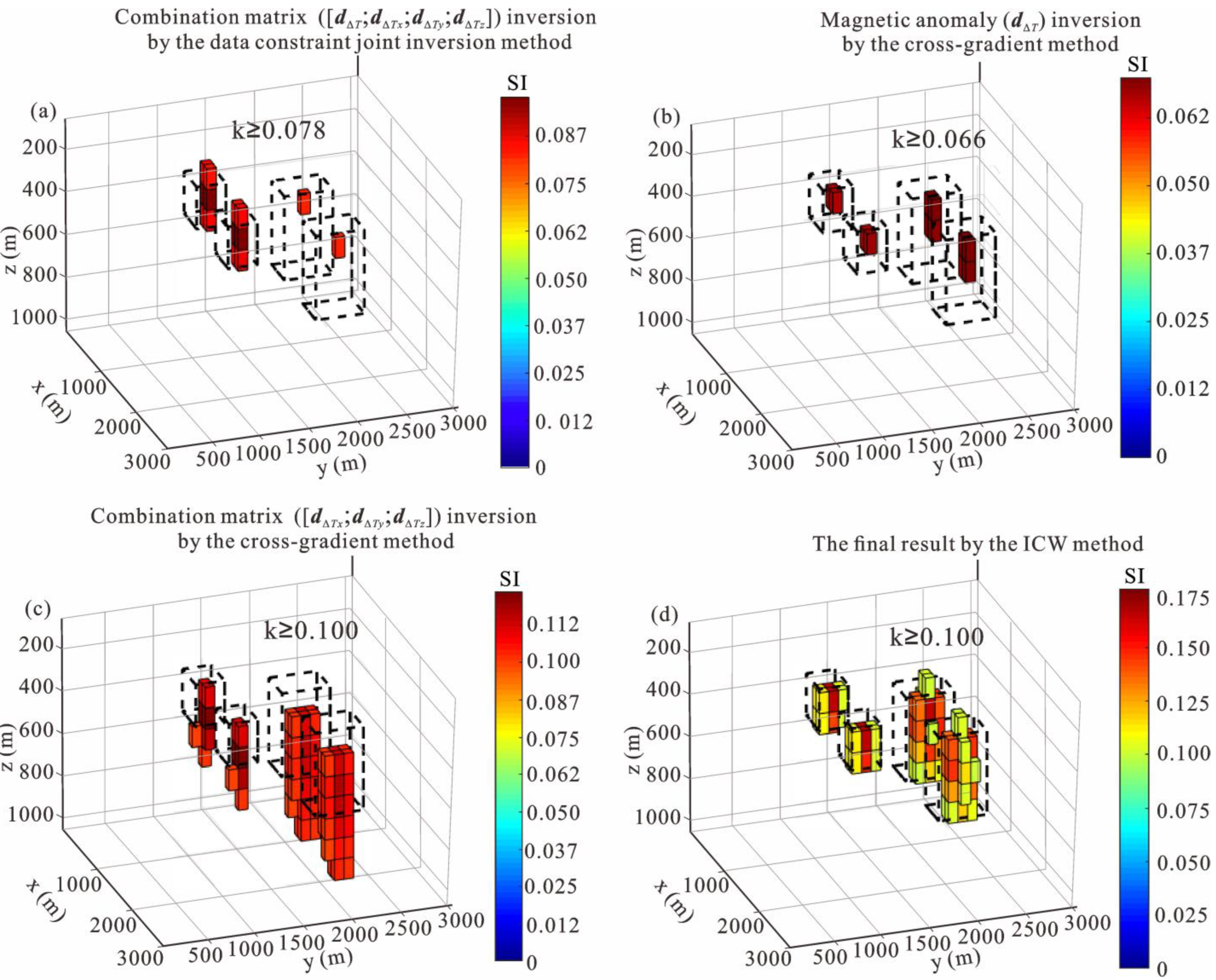
Figure 10a shows the volume-rendered image of the combination matrix inversion by the data constraint joint inversion method with magnetic susceptibility value larger than 0.078. The data constraint joint inversion has better recovery for shallow geological bodies. Nevertheless, it is quite different from the actual situation. Figure 10b shows the volume-rendered image of the magnetic anomaly inversion by the cross-gradient method. Compared with Figure 10a, the magnetic susceptibility distributions of the deep and shallow parts are more accurate but are more different from the true magnetic susceptibility value. Figure 10c shows the volume-rendered images of the combination matrix ( [ d Δ T ; d Δ T x ; d Δ T y ] ) inversion by the cross-gradient method with a magnetic susceptibility larger than 0.1 and a low vertical resolution of the magnetic susceptibility distribution. Figure 10d shows the volume-rendered images of the final result by the ICW method with a value of magnetic susceptibility larger than 0.1. The resolution and precision of the inversion results are higher, the recovered magnetic susceptibility distribution is concentrated, there is a distinct boundary of physical property, and the value of magnetic susceptibility is more similar to the true magnetic susceptibility.

4. Real Data Application

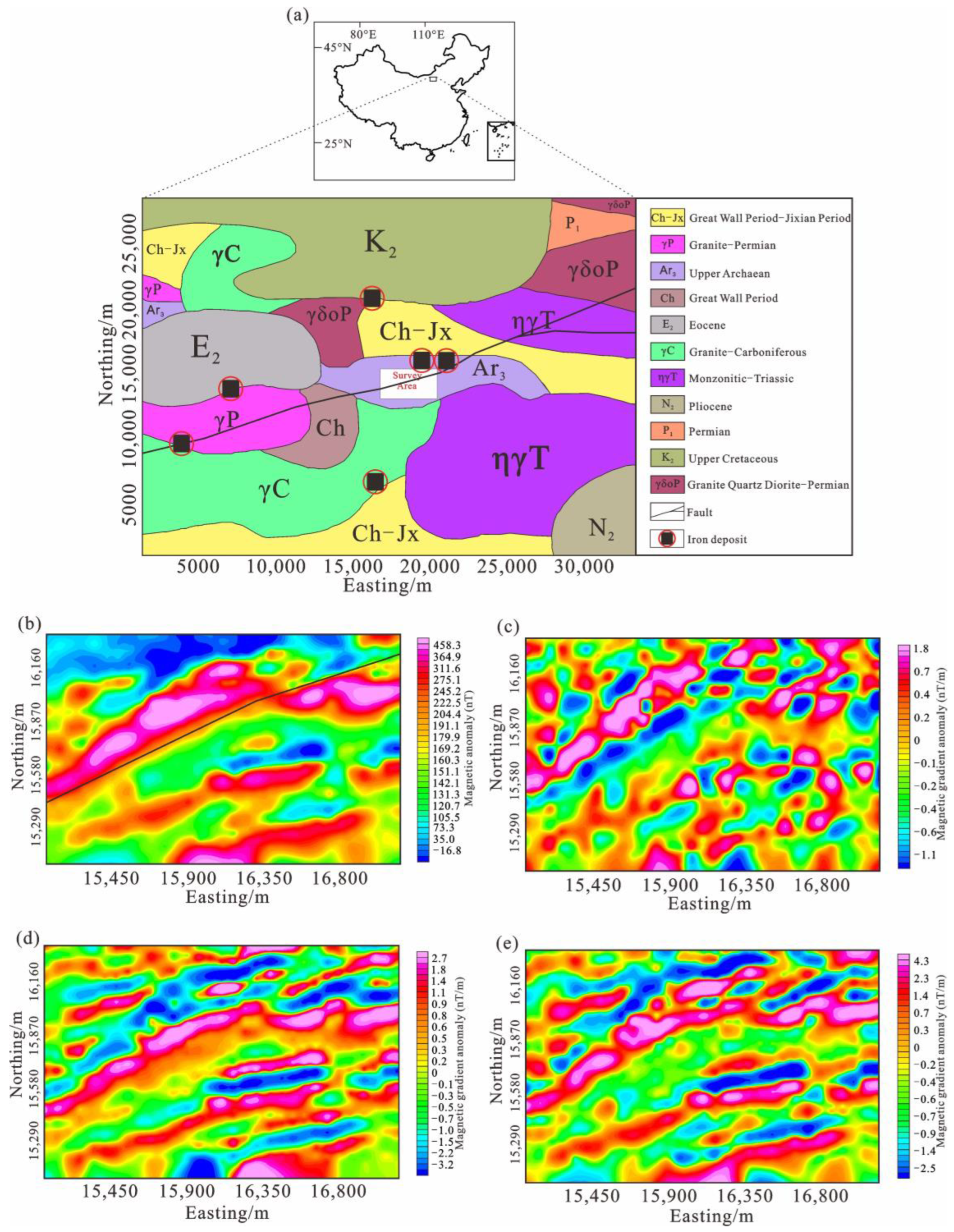
Zhurihe is in the central part of the Inner Mongolia Autonomous Region, China, which is located on the northern margin of the North China Plate and spans two major tectonic units: the North China Craton and Central Asian Orogenic Belt. Bordered by the Bayan Obo-Chifeng fault, with the North China Craton in the south and the Xing–Meng orogenic belt in the north, the Zhurihe area has undergone complicated accretionary orogenic processes and multistage tectonic deformation events, and its tectonic evolution is very complicated [41,42,43]. There are different rock types and genetic types, including Triassic monzogranite, Permian granite quartz diorite, Carboniferous granite, and Permian granite [44]. Figure 11a shows the geological map of the survey area and its surrounding areas.
To clarify the position and range of regional metal mineral resources and aeromagnetic and gradient surveys were carried out outside the current mining area from April to July 2019. The distances between the survey lines and the survey points were 100 m and 40 m, respectively. The average flight height was 100 m, and the measurement error of the aeromagnetic field and its gradient anomaly was 1.91 nT and 0.02 nT/m, respectively. Aeromagnetic anomalies and gradient anomalies in the x , y , and z -directions are shown in Figure 11b–e. The aeromagnetic and gradient anomalies are mainly distributed in the northeast direction, and the direction of the survey line is distributed in the north-south direction. The scope of the survey area is 2250 × 1470 m.
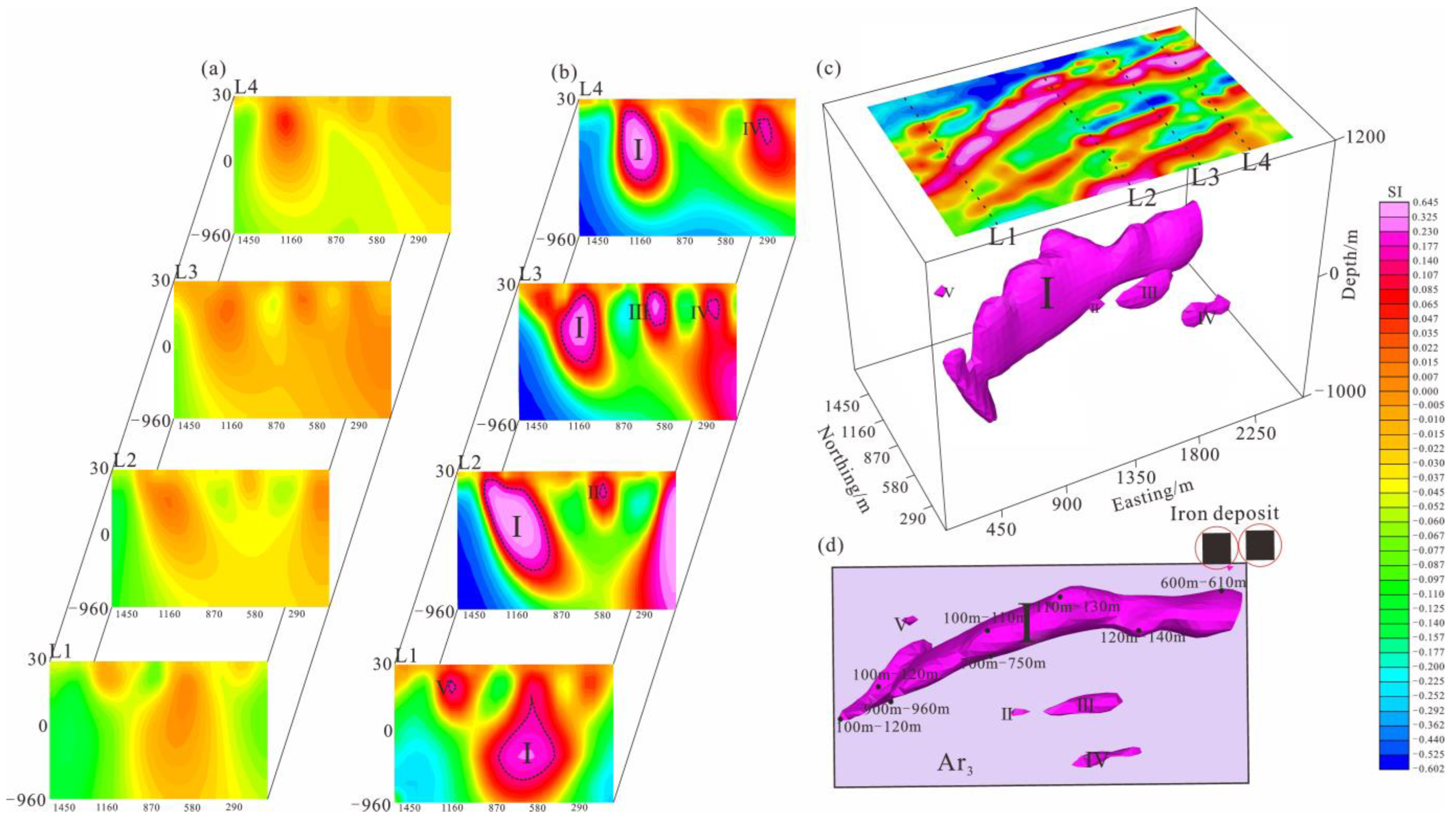
According to World Magnetic Model (WMM) 2015, the inclination and declination are 59° and −3°, respectively. The ICW method is used to carry out the joint inversion of aeromagnetic and gradient data. Slices were cut to analyze the characteristics of ore body trends. In Figure 12a, L1–L4 are the 4 slices extracted from the 3D inversion results by the data constraint joint inversion of the combination matrix ( d Δ T ; d Δ T x ; d Δ T y ; d Δ T z ). The value of magnetic susceptibility recovered from the inversion result is low, making it difficult to delineate high magnetic bodies. In Figure 12b, L1–L4 are the 4 slices extracted from the 3D inversion results by the ICW method, and the dashed circle represents the magnetic susceptibility distribution with a magnetic susceptibility larger than 0.15. In Figure 12b, high magnetic body I inclines toward the south, especially in L2, with a larger inclination angle and wider extension. Therefore, we believe that I is the mining area with the most mining potential. Figure 12c shows the 3D inversion result by the ICW method with a magnetic susceptibility larger than 0.15. The inversion results indicate that the survey area mainly contains one large high magnetic body and four small high magnetic bodies. The volume of high magnetic body I is the largest, distributed in the northeast direction, and the top burial depth and bottom burial depth are 100 m and 960 m, respectively. Figure 12c shows that the largest high-value area is affected by the fault, which corresponds to high magnetic body I, so we infer that high magnetic body I is a large intrusive deposit. The depth of high magnetic bodies II and III is 180 m, the depth of high magnetic body IV is 200 m, and the depth of high magnetic body V is 100 m. Compared with magnetic body I, these high-magnetic bodies are smaller in volume, shallower in depth, and have minimal mining potential.
Figure 12d shows the horizontal distribution of high magnetic bodies. The depth range of certain areas of high magnetic body I has been given, which has important guiding information for the future exploration and development of deep concealed ore bodies.

5. Conclusions

We developed a joint magnetic susceptibility inversion method for aeromagnetic and gradient data named the intersection constraint weighting (ICW) method. The resolution and precision of inversion results were enhanced by gradually increasing the gradient data and by normalizing the inversion results as weight functions and through the cross-use of weight function. Theoretical model tests proved that the ICW method could effectively improve the resolution and precision of inversion results. The magnetic susceptibility distribution is more consistent with the real magnetic susceptibility. In the theoretical model tests, the precision of the ICW method can be improved by 25% more than conventional inversion methods. Simultaneously, the ICW method also has strong anti-noise ability and stability. In real data applications, the High-Resolution inversion result obtained by the ICW method can be used to accurately delineate the strike characteristics of near-surface and deep magnetic sources and to determine the mining area with the most mining potential. The inversion result has good practical value for searching for regional magnetite deposits.

Author Contributions

Conceptualization, G.M.; methodology, G.M.; software, J.C.; validation, J.C. and L.L.; formal analysis, J.C.; data curation, J.C.; writing—original draft preparation, J.C.; writing—review and editing, L.L.; visualization, G.M.; supervision, G.M.; project administration, G.M.; funding acquisition, L.L. All authors have contributed significantly and have participated sufficiently to take responsibility for this research. All authors have read and agreed to the published version of the manuscript.

Funding

This research is supported by the National Natural Science Foundation of China (Grant Number: 42174166).

Data Availability Statement

Not applicable.

Conflicts of Interest

The author declare that they have no conflict of interest.

References

  1. Wang, J.; Meng, X.H. An aeromagnetic investigation of the Dapai deposit in Fujian Province, South China: Structural and mining implications. Ore Geol. Rev. 2019, 112, 103061. [Google Scholar] [CrossRef]
  2. Gao, X.H.; Xiong, S.Q.; Yu, C.C.; Zhang, D.H.; Wu, C.P. The estimation of magnetite prospective resources based on aeromagnetic data: A case study of Qihe Area, Shandong Province, China. Remote Sens. 2021, 13, 1216. [Google Scholar] [CrossRef]
  3. Wasilewski, P.; Fountain, D.W. The Ivrea Zone as a model for the distribution of magnetization in the continental crust. Geophys. Res. Lett. 1982, 9, 333–336. [Google Scholar] [CrossRef]
  4. Schnetzler, C.C. An estimation of continental crust magnetization and susceptibility from Magsat data for the conterminous United States. J. Geophys. Res.-Sol. Earth 1985, 90, 2617–2620. [Google Scholar] [CrossRef]
  5. Woodward, D.J. Inversion of aeromagnetic data using digital terrain models. Geophysics 1993, 58, 645–652. [Google Scholar] [CrossRef]
  6. Batista-Rodríguez, J.A.; Pérez-Flores, M.A.; Quiroga-Goode, G.; Gallardo, L.A. Geometry of ophiolites in eastern Cuba from 3D inversion of aeromagnetic data, constrained by surface geology. Geophysics 2007, 72, B81–B91. [Google Scholar] [CrossRef]
  7. Liu, S.; Hu, X.Y.; Liu, T.Y.; Feng, J.; Gao, W.L.; Qiu, L.Q. Magnetization vector imaging for borehole magnetic data based on magnitude magnetic anomaly. Geophysics 2013, 78, D429–D444. [Google Scholar] [CrossRef]
  8. Anderson, E.D.; Zhou, W.; Li, Y.G.; Hitzman, M.W.; Monecke, T.; Lang, J.R.; Kelley, K.D. Three-dimensional distribution of igneous rocks near the Pebble porphyry Cu−Au−Mo deposit in southwestern Alaska: Constraints from regional-scale aeromagnetic data. Geophysics 2014, 79, B63–B79. [Google Scholar] [CrossRef]
  9. Bott, M.H.P. Solution of the linear inverse problem in magnetic interpretation with application to oceanic magnetic anomalies. Geophys. J. Int. 1957, 13, 313–323. [Google Scholar] [CrossRef] [Green Version]
  10. Arkani-Hamed, J.; Strangway, D.W. Magnetic susceptibility anomalies of lithosphere beneath eastern Europe and the Middle East. Geophysics 1986, 51, 1711–1724. [Google Scholar] [CrossRef]
  11. Li, Y.G.; Oldenburg, D.W. 3-D inversion of magnetic data. Geophysics 1996, 61, 394–408. [Google Scholar] [CrossRef]
  12. Pilkington, M. 3-D magnetic imaging using conjugate gradients. Geophysics 1997, 62, 1132–1142. [Google Scholar] [CrossRef]
  13. Li, Y.G.; Oldenburg, D.W. Fast inversion of large-scale magnetic data using wavelet transforms and a logarithmic barrier method. Geophys. J. Int. 2003, 152, 251–265. [Google Scholar] [CrossRef] [Green Version]
  14. Pilkington, M. 3D magnetic data-space inversion with sparseness constraints. Geophysics 2009, 74, L7–L15. [Google Scholar] [CrossRef]
  15. Li, W.B.; Qian, J.L.; Li, Y.G. Joint inversion of surface and borehole magnetic data: A level-set approach. Geophysics 2020, 85, J15–J33. [Google Scholar] [CrossRef]
  16. Paoletti, V.; Fedi, M.; Italiano, F.; Florio, G.; Ialongo, S. Inversion of gravity gradient tensor data: Does it provide better resolution? Geophys. J. Int. 2016, 205, 192–202. [Google Scholar] [CrossRef] [Green Version]
  17. Zhdanov, M.S.; Robert, E.; Souvik, M. Three-dimensional regularized focusing inversion of gravity gradient tensor component data. Geophysics 2004, 69, 925–937. [Google Scholar] [CrossRef]
  18. Meng, Z.H. 3D inversion of full gravity gradient tensor data using SL0 sparse recovery. J. Appl. Geophys. 2016, 127, 112–128. [Google Scholar] [CrossRef]
  19. Qin, P.B.; Zhang, C.; Meng, Z.H.; Zhang, D.L.; Hou, Z.L. Three integrating methods for gravity and gravity gradient 3-D inversion and their comparison based on a new function of discrete stability. IEEE Trans. Geosci. Remote Sens. 2022, 60, 1–12. [Google Scholar] [CrossRef]
  20. Martinez, C.Y.; Li, Y. Inversion of regional gravity gradient data over the Vredefort Impact Structure, South Africa. In Proceedings of the 81st SEG Annual International Meeting, San Antonio, CA, USA, 18–23 September 2011; pp. 841–845. [Google Scholar]
  21. Capriotti, J.; Li, Y.; Krahenbuhl, R. Joint inversion of gravity and gravity gradient data using a binary formulation: GEM Chengdu 2015. In Proceedings of the International Workshop and Gravity, Electrical & Magnetic Methods and Their Applications, Chengdu, China, 19–22 April 2015; pp. 326–329. [Google Scholar]
  22. Qin, P.B.; Xiang, M.; Liang, X.; Hou, Z.L. A new method to integrate different gravity gradient components in reweighted regularized inversion with a minimum support constraint. Geophys. J. Int. 2019, 217, 1387–1412. [Google Scholar] [CrossRef]
  23. Hood, P. Gradient measurement in aeromagnetic survey. Geophysics 1965, 30, 891–902. [Google Scholar] [CrossRef]
  24. Barongo, J.O. Method for depth estimation on aeromagnetic vertical gradient anomalies. Geophysics 1985, 50, 963–968. [Google Scholar] [CrossRef]
  25. Oruç, B.; Keskinsezer, A. Detection of causative bodies by normalized full gradient of aeromagnetic anomalies from east Marmara region, NW Turkey. J. Appl. Geophys. 2008, 65, 39–49. [Google Scholar] [CrossRef]
  26. Beiki, M.; Clark, D.A.; Austin, J.R.; Foss, C.A. Estimating source location using normalized magnetic source strength calculated from magnetic gradient tensor data. Geophysics 2012, 77, J23–J37. [Google Scholar] [CrossRef] [Green Version]
  27. Li, L.; Guo, H.; Wang, P.; Jia, W.J. Research on RTP aeromagnetic gradient data and its applicability in different latitudes. Appl. Geophys. 2016, 13, 48–58. [Google Scholar] [CrossRef]
  28. Brahimi, S.; Maire, P.L.; Ghienne, J.F.; Munschy, M. Deciphering channel networks from aeromagnetic potential field data: The case of the North Sea Quaternary tunnel valleys. Geophys. J. Int. 2020, 220, 1447–1462. [Google Scholar] [CrossRef]
  29. Davis, K.; Li, Y.G. Joint processing of total-field and gradient magnetic data. Explor. Geophys. 2011, 42, 199–206. [Google Scholar] [CrossRef]
  30. Gallardo, L.A.; Meju, M.A. Characterization of heterogeneous near-surface materials by joint 2D inversion of dc resistivity and seismic data. Geophys. Res. Lett. 2003, 30, 1658. [Google Scholar] [CrossRef]
  31. Gallardo, L.A.; Meju, M.A. Joint two-dimensional DC resistivity and seismic travel time inversion with cross-gradients constraints. J. Geophys. Res.-Sol. Earth 2004, 109, B03311. [Google Scholar] [CrossRef]
  32. Linde, N.; Binley, A.; Tryggvason, A.; Pedersen, L.B.; Revil, A. Improved hydrogeophysical characterization using joint inversion of cross-hole electrical resistance and ground-penetrating radar traveltime data. Water Resour. Res. 2006, 42, W12404. [Google Scholar] [CrossRef]
  33. Fregoso, E.; Gallardo, L.A. cross-gradients joint 3D inversion with applications to gravity and magnetic data. Geophysics 2009, 74, L31–L42. [Google Scholar] [CrossRef]
  34. Gross, L. Weighted cross-gradient function for joint inversion with the application to regional 3-D gravity and magnetic anomalies. Geophys. J. Int. 2019, 217, 2035–2046. [Google Scholar] [CrossRef]
  35. Vatankhah, S.; Liu, S.; Renaut, R.A.; Hu, X.Y. An efficient alternating algorithm for the Lp-norm cross-gradient joint inversion of gravity and magnetic data using the 2-D fast fourier transform. IEEE Trans. Geosci. Remote Sens. 2020, 60, 1–16. [Google Scholar] [CrossRef]
  36. Tavakoli, M.; Kalateh, A.N.; Rezaie, M.; Gross, L. Sequential joint inversion of gravity and magnetic data via the cross-gradient constraint. Geophys. Prospect. 2021, 69, 1542–1559. [Google Scholar] [CrossRef]
  37. Lawson, L.C.; Hanson, J.R. Solving Least-Squares Problems; Prentice-Hall: Englewood Cliffs, NJ, USA, 1974. [Google Scholar]
  38. Portniaguine, O.; Zhdanov, M.S. Focusing geophysical inversion images. Geophysics 1999, 64, 874–887. [Google Scholar] [CrossRef] [Green Version]
  39. Li, Y.G.; Oldenburg, D.W. Joint inversion of surface and Three-component borehole magnetic data. Geophysics 2000, 65, 540–552. [Google Scholar] [CrossRef]
  40. Paoletti, V.; Hansen, P.C.; Hansen, M.F.; Fedi, M. A computationally efficient tool for assessing the depth resolution in potential–field inversion. Geophysics 2014, 79, A33–A38. [Google Scholar] [CrossRef]
  41. Xiao, W.J.; Windley, B.F.; Hao, J.; Zhai, M.G. Accretion leading to collision and the Permian Solonker suture, Inner Mongolia, China: Termination of the central Asian orogenic belt. Tectonics 2003, 22, 1069–1089. [Google Scholar] [CrossRef] [Green Version]
  42. Jian, P.; Liu, D.; Kröner, A.; Windley, B.F.; Shi, Y.; Zhang, F.; Shi, G.; Miao, L.; Zhang, W.; Zhang, Q. Time scale of an early to mid-Paleozoic orogenic cycle of the long-lived Central Asian Orogenic Belt, Inner Mongolia of China: Implications for continental growth. Lithos 2008, 101, 233–259. [Google Scholar] [CrossRef]
  43. Jian, P.; Liu, D.Y.; Kroner, A.; Windley, B.F.; Shi, Y.R.; Zhang, W.; Zhang, F.Q.; Miao, L.C.; Zhang, L.Q.; Tomurhuu, D. Evolution of a Permian intraoceanic arc-trench system in the Solonker suture zone, Central Asian Orogenic Belt, China and Mongolia. Lithos 2010, 118, 169–190. [Google Scholar] [CrossRef]
  44. Sun, J.; Zhu, X.K.; Chen, Y.L.; Fang, N. Iron isotopic constraints on the genesis of Bayan Obo ore deposit, Inner Mongolia, China. Precambrian Res. 2013, 235, 88–106. [Google Scholar] [CrossRef]
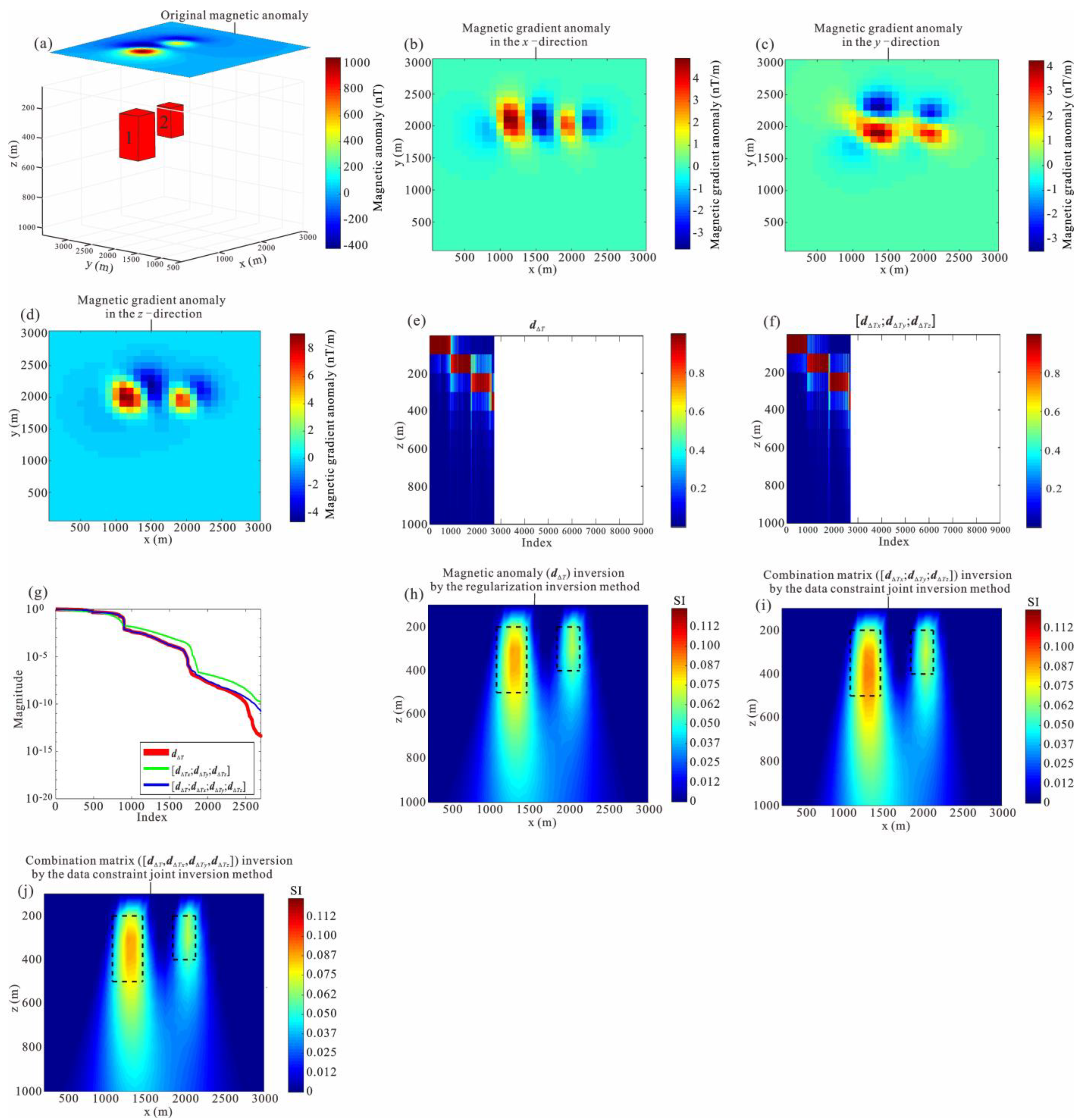
Figure 1. DRP, eigenvalue spectra for kernel function matrices and magnetic susceptibility slices ( y = 1900 m) obtained by magnetic anomaly ( d Δ T ) inversion and combination matrix ( d Δ T x ; d Δ T y ; d Δ T z ) inversion. (a) 3D view of 2 prisms and magnetic anomaly. (b) Magnetic gradient anomaly in the x -direction. (c) Magnetic gradient anomaly in the y -direction. (d) Magnetic gradient anomaly in the z -direction. (e,f) DRP of the magnetic anomaly and combination matrix of magnetic gradient anomalies. (g) Eigenvalue spectra for kernel function matrices. (h) Magnetic anomaly ( d Δ T ) inversion by the regularization inversion method. (i) Combination matrix ( d Δ T x ; d Δ T y ; d Δ T z ) inversion by the data constraint joint inversion method. (j) Combination matrix ( d Δ T ; d Δ T x ; d Δ T y ; d Δ T z ) inversion by the data constraint joint inversion method.
Remotesensing 14 06029 g001
Figure 2. DRP, eigenvalue spectra for kernel function matrices and magnetic susceptibility slices ( y = 1900 m) obtained by magnetic anomaly ( d Δ T ) inversion and combination matrix ( d Δ T x ; d Δ T y ; d Δ T z ) inversion. (a) 3D view of 2 prisms and magnetic anomaly. (b) Magnetic gradient anomaly in the x -direction. (c) Magnetic gradient anomaly in the y -direction. (d) Magnetic gradient anomaly in the z -direction. (e,f) DRP of the magnetic anomaly and combination matrix of magnetic gradient anomalies. (g) Eigenvalue spectra for kernel function matrices. (h) Magnetic anomaly ( d Δ T ) inversion by the regularization inversion method. (i) Combination matrix ( d Δ T x ; d Δ T y ; d Δ T z ) inversion by the data constraint joint inversion method. (j) Combination matrix ( d Δ T ; d Δ T x ; d Δ T y ; d Δ T z ) inversion by the data constraint joint inversion method.
Remotesensing 14 06029 g002
Figure 3. Magnetic and gradient anomalies and magnetic susceptibility slices ( y = 1900 m) obtained by different inversion methods. (a) 3D view of 2 prisms and magnetic anomaly. (b) Magnetic gradient anomaly in the x -direction. (c) Magnetic gradient anomaly in the y -direction. (d) Magnetic gradient anomaly in the z -direction. (e) Magnetic susceptibility slice ( y = 1900 m) obtained by regularization inversion of the magnetic anomaly ( d Δ T ). (f) Magnetic susceptibility slice ( y = 1900 m) by data constraint joint inversion of the combination matrix ( d Δ T x ; d Δ T y ; d Δ T z ). (g) Magnetic susceptibility slice ( y = 1900 m) by data constraint joint inversion of the combination matrix ( d Δ T ; d Δ T x ; d Δ T y ; d Δ T z ). (h) Magnetic susceptibility slice ( y = 1900 m) by cross-gradient inversion of the magnetic anomaly ( d Δ T ). (i) Magnetic susceptibility slice ( y = 1900 m) by cross-gradient inversion of the combination matrix ( d Δ T x ; d Δ T y ; d Δ T z ).
Remotesensing 14 06029 g003
Figure 4. Flowchart of the ICW method.
Remotesensing 14 06029 g004
Figure 5. Magnetic susceptibility slice ( y = 1900 m) and volume-rendered images by the ICW method. (a) Magnetic susceptibility slice ( y = 1900 m) of the first stage of magnetic anomaly ( d Δ T ) inversion by the ICW method. (b) Magnetic susceptibility slice ( y = 1900 m) of the first stage of combination matrix ( [ d Δ T ; d Δ T x ] ) inversion by the ICW method. (c) volume-rendered image of the combination matrix ( [ d Δ T ; d Δ T x ] ) inversion of the first stage by the ICW method. (d) Magnetic susceptibility slice ( y = 1900 m) of the second stage of magnetic anomaly ( d Δ T ) inversion by the ICW method. (e) Magnetic susceptibility slice ( y = 1900 m) of the second stage of combination matrix ( [ d Δ T ; d Δ T x ; d Δ T y ] ) inversion by the ICW method. (f) volume-rendered image of the combination matrix ( [ d Δ T ; d Δ T x ; d Δ T y ] ) inversion of the second stage by the ICW method. (g) Magnetic susceptibility slice ( y = 1900 m) of the final result by the ICW method. (h) volume-rendered image of the final result by the ICW method.
Remotesensing 14 06029 g005
Figure 6. Magnetic and gradient anomalies (compared with the model in Figure 2, the buried depths of the prisms are increased by 100 m) and the volume-rendered images by different methods. (a) 3D view of 2 prisms and magnetic anomaly. (b) Magnetic gradient anomaly in the x -direction. (c) Magnetic gradient anomaly in the y -direction. (d) Magnetic gradient anomaly in the z -direction. (e) volume-rendered image of the combination matrix ( [ d Δ T ; d Δ T x ; d Δ T y ; d Δ T z ] ) inversion by the data constraint joint inversion method. (f) volume-rendered image of magnetic anomaly ( d Δ T ) inversion by the cross-gradient method. (g) volume-rendered image of combination matrix ( [ d Δ T ; d Δ T x ; d Δ T y ] ) inversion by the cross-gradient method. (h) volume-rendered image of the final result by the ICW method.
Remotesensing 14 06029 g006
Figure 7. Magnetic and gradient anomalies with Gaussian noise and volume-rendered images by different inversion methods. (ad) Noise–corrupted magnetic and gradient anomalies with Gaussian noise of a signal-to-noise ratio of 20. (e) volume-rendered image of combination matrix ( [ d Δ T ; d Δ T x ; d Δ T y ; d Δ T z ] ) inversion by the data constraint joint inversion method. (f) volume-rendered image of magnetic anomaly ( d Δ T ) inversion by the cross-gradient method. (g) volume-rendered image of the combination matrix ( [ d Δ T ; d Δ T x ; d Δ T y ] ) inversion by the cross-gradient method. (h) volume-rendered image of the final result by the ICW method.
Remotesensing 14 06029 g007
Figure 8. Magnetic and gradient anomalies with Gaussian noise and volume-rendered images by different inversion methods. (ad) Noise–corrupted magnetic and gradient anomalies with Gaussian noise of a signal-to-noise ratio of 10. (e) volume-rendered image of combination matrix ( [ d Δ T ; d Δ T x ; d Δ T y ; d Δ T z ] ) inversion by the data constraint joint inversion method. (f) volume-rendered image of magnetic anomaly ( d Δ T ) inversion by the cross-gradient method. (g) volume-rendered image of the combination matrix ( [ d Δ T ; d Δ T x ; d Δ T y ] ) inversion by the cross-gradient method. (h) volume-rendered image of the final result by the ICW method.
Remotesensing 14 06029 g008
Figure 9. 3D view of the 4 prisms and corresponding magnetic and gradient anomalies. (a) 3D view of the 4 models and the magnetic anomaly. (b) Magnetic gradient anomaly in the x -direction. (c) Magnetic gradient anomaly in the y -direction. (d) Magnetic gradient anomaly in the z -direction.
Remotesensing 14 06029 g009
Figure 10. volume-rendered images by different inversion methods. (a) volume-rendered image of the combination matrix ( [ d Δ T ; d Δ T x ; d Δ T y ; d Δ T z ] ) inversion by the data constraint joint inversion method. (b) volume-rendered image of magnetic anomaly ( d Δ T ) inversion by the cross-gradient method. (c) volume-rendered image of combination matrix ( [ d Δ T ; d Δ T x ; d Δ T y ] ) inversion by the cross-gradient method. (d) volume-rendered image of the final result by the ICW method.
Remotesensing 14 06029 g010
Figure 11. Geographical location and geological conditions and the measured aeromagnetic and gradient anomalies. (a) Geographical location and geological conditions of the survey area. (b) Measured aeromagnetic anomaly. (c) Measured aeromagnetic gradient anomaly in the x -direction. (d) Measured aeromagnetic gradient anomaly in the y -direction. (e) Measured aeromagnetic gradient anomaly in the z -direction.
Remotesensing 14 06029 g011
Figure 12. Inversion result of the measured data. (a) Magnetic susceptibility slice by the data constraint joint inversion of the combination matrix ( [ d Δ T ; d Δ T x ; d Δ T y ; d Δ T z ] ). (b) Magnetic susceptibility slice by the ICW method. (c) 3D inversion result by the ICW method. (d) Horizontal range distribution of the high magnetic body.
Remotesensing 14 06029 g012
Publisher’s Note: MDPI stays neutral with regard to jurisdictional claims in published maps and institutional affiliations.