Abstract
The emerging WiFi Round Trip Time measured by the IEEE 802.11mc standard promised sub-meter-level accuracy for WiFi-based indoor positioning systems, under the assumption of an ideal line-of-sight path to the user. However, most workplaces with furniture and complex interiors cause the wireless signals to reflect, attenuate, and diffract in different directions. Therefore, detecting the non-line-of-sight condition of WiFi Access Points is crucial for enhancing the performance of indoor positioning systems. To this end, we propose a novel feature selection algorithm for non-line-of-sight identification of the WiFi Access Points. Using the WiFi Received Signal Strength and Round Trip Time as inputs, our algorithm employs multi-scale selection and Machine Learning-based weighting methods to choose the most optimal feature sets. We evaluate the algorithm on a complex campus WiFi dataset to demonstrate a detection accuracy of 93% for all 13 Access Points using 34 out of 130 features and only 3 s of test samples at any given time. For individual Access Point line-of-sight identification, our algorithm achieved an accuracy of up to 98%. Finally, we make the dataset available publicly for further research.
1. Introduction
Although GPS has been indispensable for outdoor positioning, robust indoor positioning remains a research challenge. First, modern buildings with complex interiors make it difficult for the weak GPS signals to penetrate. Second, the 5–10 m GPS accuracy cannot provide the indoor users with the positioning accuracy they need for room-level tracking. To address these challenges, several technologies were proposed in the literature and applied in the real world [1]. Due to the ubiquity of WiFi-enabled devices, WiFi-based indoor positioning has drawn much attention. Indoor positioning systems using the WiFi Received Signal Strength (RSS) were widely reported to achieve 2–3 m accuracy on average [2,3]. However, the challenges for WiFi RSS-based systems were signal instability and spatial ambiguity caused by the multipath interference [4].
In recent years, the introduction of WiFi Round Trip Time (RTT) from the IEEE 802.11mc standard, which measures the travelling time of the signal between the transmitter and receiver, has promised sub-meter positioning accuracy, under the assumption of a clear line-of-sight (LOS) path. With RTT, positioning systems could trilaterate the user’s location, assuming that the signal measure reflects the true distance. However, workplaces with plenty of furniture often do not have a clear LOS path from the WiFi Access Points to most locations, and hence, impact the wireless signal’s integrity. In such environments, the WiFi RSS and RTT signals could be attenuated, reflected, blocked, or interfered, and resulted in fluctuating and unpredictable measures [5]. Since the WiFi signal travels at the speed of light, the fluctuating and reflecting nature of RTT propagation in complex indoor spaces would result in large positioning errors with the trilateration technique. Moreover, the instability of WiFi signal measures in non-line-of-sight (NLOS) scenarios would create highly similar values of WiFi measurements in two distinguishing locations several meters away. Such similarity of signal measures would greatly decrease the accuracy of WiFi fingerprinting in complex indoor environments. Therefore, detecting the LOS condition of the WiFi Access Points is of great importance in enhancing the system performance.
To this end, we propose a framework for WiFi LOS detection by automatically selecting the most informative feature set using Machine Learning and weighting methods. For further optimization, we develop a novel multi-scale selection (MSS) method to validate the importance of the features on multiple scales. The proposed framework used the correlation between the input features and ground-truth labels to decide the importance of each feature. To further investigate the informativity of the features, datasets of different sampling sizes are used for feature validation.
In the preprocessing stage of the proposed framework, statistics of the input WiFi RSS and RTT measurements were computed and fed into an importance filter. Several popular feature selection models were used in the importance filter to decide their own feature set based on different algorithms. Then, statistical features chosen by feature selection models were assigned initial weights based on their macro F1 score and accuracy in LOS identification. To validate the selected features from both macroscopical and microscopical perspectives, multi-sampling datasets were introduced. Based on the performance of the selected feature set, weights adjustment was leveraged to reselect the features recursively. To evaluate the performance and transferability of the proposed algorithm, a large-scale real-world campus building floor was used as the testbed. Each location in the dataset was manually labeled and verified for ground truth. Since the framework only focuses on reducing high-dimensional data based on the relevance between input signal measures and the output, it could be applied to other signal measurements in indoor positioning.
The article’s contributions are summarized as follows:
- A novel feature selection framework was proposed to identify the LOS conditions of WiFi APs with high accuracy even with few data samples, while using fewer Machine Learning features than existing state-of-the-arts.
- A large-scale real-world dataset for a campus floor was collected and made available for further research. To the best of our knowledge, this was the first publicly available dataset that contains both WiFi RSS and RTT signal measures, as well as LOS conditions of each AP for every location.
- We analyzed our framework on such dataset to evaluate the efficiency and to provide a baseline performance for further research.
The rest of the article is organized as follows: Section 2 introduces the related work in WiFi LOS identification. Section 3 provides a detailed description of the framework architecture, then the data preprocessing and the proposed feature selection method is investigated in Section 4, the experimental setup and empirical performance are presented and analyzed in Section 5. Finally, Section 7 concludes our work and outlines future work.
2. Related Work
The Non-Line-of-Sight (NLOS) scenario has always been a challenge for most positioning systems. For instance, although promising positioning accuracy is provided by the Global Navigation Satellite System (GNSS) [6,7,8,9,10] in most outdoor spaces, GPS still struggles where the signals are interfered by skyscrapers and poor weather conditions. To address the problem, the system proposed by [11] leveraged the vector tracking loop (VTL) to detect NLOS and perform corrections. Features such as noise bandwidth, time delay of multi-correlator peaks, and code discriminator outputs were used as the input data.
Similarly, Massive Multiple-Input Multiple-Output (MIMO) systems also suffered from the same NLOS challenge [12,13,14,15,16]. In [17], indoor MIMO channel measures were analyzed for kurtosis-based LOS detection. The importance of introducing kurtosis statistical features was investigated based on channel impulse response (CIR). A stochastic model was developed in [18] for outdoor LOS/NLOS scenarios. Multipath components (MPCs) extracted from sub-array outputs were assessed and identified into spatial-stationary (SS) for modelling. To improve the vehicle MIMO localisation systems, Support Vector Machines for LOS identification was proposed to process CIR information [19]. The role of small cells was investigated in [20] for optimizing downlink heterogeneous cellular networks under LOS and NLOS transmissions. Beside using a convolutional neural network (CNN) in a 3-D massive MIMO channel model, LOS detection [21,22] treated the problem as a binary hypothesis test. Based on time-space-frequency channel correlation, the system in [22] aimed to improve the new radio capacity and spectral efficiency of the 5G network.
For ultra-wideband systems (UWB), in ideal LOS conditions, the positioning accuracy was widely reported to be at the centimeter level [23,24,25,26,27]. Researchers have also attempted to address NLOS conditions for UWB indoor spaces. In [28], recursive decision tree learning was used to exploit the UWB data for LOS detections. The CIR information extracted from UWB signals was taken into consideration. Machine Learning methods were leveraged to mitigate for the deviation of NLOS UWB measurements [29]. In [30], multi-layer perceptron and CNN were used to make predictions. The 2D Time Difference of Arrival (TDoA) framework based on deep Q-learning was proposed in [31] to make efficient LOS node selection. The system in [32] introduced Morlet wave transform (MWT)to make LOS detection based on time-domain characteristics. Table 1 compares the performance of LOS identification in different systems.

Table 1.
Comparison of the performance of notable work in LOS identification.
Despite its high accuracy, the disadvantage of UWB positioning systems is that they use proprietary beacons. On the contrary, WiFi-based indoor positioning systems leverage existing WiFi APs. To achieve high LOS identification, Channel State Information (CSI) was used [2,33,34,35,36,37]. A detailed description of the channel properties could be extracted from CSI to identify the propagation situation of the WiFi signal [38]. Phase information, amplitude information, Time-of-flight (ToF), and Angle-of-arrival (AoA) [39] extracted from CSI were commonly used as inputs to identify LOS conditions. Similar to MIMO and UWB systems, CIR converted by Inverse Fast Fourier Transform (IFFT) also helped improve the identification accuracy [40,41,42]. In [40], the system achieved 90.5% LOS identification accuracy when using Rician-K and skewness derived from CSI. The root mean square delay spread, Skewness, Kurtosis of CSI were used in [43] in making LOS detection with an accuracy of 95%. Systems proposed in [44,45] investigated the potential of power-delay profile and power-angle spectrum, respectively. Other than exploiting phase information of each sub-carrier [41], statistics of CIR were also studied for their performance in making LOS classifications [46,47,48,49,50,51]. The system proposed by [47] achieved detection of LOS AP with an accuracy of up to 94%. The standard deviation, kurtosis and skewness of CIR were used in [46] and delivered an accuracy of 95% in detecting LOS situation. Furthermore, CSI could also be leveraged to detect human activities. The system proposed in [52] used existing WiFi equipments for location-oriented activity identification at home based on CSI signal measurement. In [53], CSI was used to detect the human respiration based on the Fresnel model. Although CSI provides detailed channel information of the WiFi signal measures and is more informative and efficient in indoor positioning, it is hard to access. CSI information could only be acquired on a PC with a modified WiFi driver such as the Intel 5300 NIC. These limitations make it challenging to use in mobile devices such as smartphones and tablets. As this article focuses on the wider implementation of WiFi-based indoor positioning on heterogeneous devices, CSI was not considered to be one of the input signal measurements in our empirical experiments, although our proposed framework could also be applied for CSI measures.
In addition to CSI, WiFi Received Signal Strength (RSS) and Round Trip Time (RTT) were often employed, due to their accessible nature in all WiFi-enabled devices. In addition, the ESP32 system also supports WiFi RSS and RTT signal measurements. ESP32 is a low-cost and low-power-consumption device integrated with a series of chips to support Wi-Fi and Bluetooth. For WiFi RTT measurement testing and collection on ESP32, a utility software called Chronos was created, as introduced in [54]. One of the most famous WiFi-based positioning techniques for WiFi RSS is fingerprinting. The more complicated the interior along the WiFi propagation path, the more unique the WiFi RSS measurements. Thus, in a real-world indoor space, each location will have its special WiFi RSS pattern. Such distinguishing WiFi RSS patterns could be leveraged by indoor positioning systems to make precise positioning estimations. As shown in Figure 1, fingerprinting consists of two phases: an offline phase and an online phase. In the offline phase, a dataset is built in the targeted testbed. WiFi measurements are recorded at each reference point and preprocessed before being stored in the dataset. Each data sample is carefully labeled with ground-truth coordinates of the reference point where the WiFi signal measures are collected. In the online phase, when the user reports a real-time WiFi RSS measurement from an unknown location, the system will match the measurement with those in the dataset and make a positioning estimation based on their relevance. Fingerprinting could also be used in WiFi RTT-based indoor positioning systems.
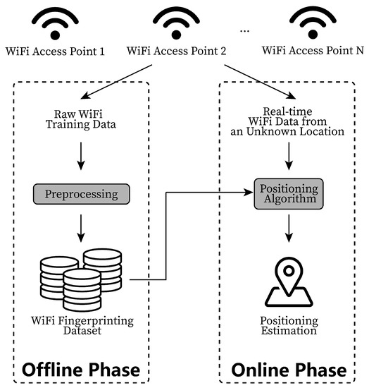
Figure 1.
The basic architecture of a classic WiFi indoor fingerprinting system. This system has two phases: the offline phase and the online phase. In the offline phase, the WiFi signal measurements are collected, preprocessed, labeled and stored in the dataset. In the online phase, the WiFi measurements received by the user from an unknown location are compared with the measurements in the database by the positioning algorithm to obtain the final location estimation.
The most common WiFi LOS identification method in the literature was based on the statistical features of the signal measures. Several works employed the Round Trip Time (RTT) [55,56,57,58,59,60], Received Signal Strength (RSS) [61,62,63,64]. The researchers in [65] used RSS in identifying LOS conditions. A Gaussian model was leveraged to make detections based on RSS signal measures in the system proposed by [66]. RTT measurements along with pedestrian dead reckoning were used in LOS identification systems in [67]. To make use of the statistics from WiFi signal measure, the standard deviations of both RSS and RTT were used in [68] for NLOS error detections. Statistical features of kurtosis and the mean value of both RSS and RTT measures were included in [69] identification system. Furthermore, a wider range of statistics was covered in the LOS and NLOS channel detection system in [70]. In addition to kurtosis and mean, skewness, hyper-skewness, and peak probability extracted from RSS measures were investigated [70]. As concluded in [71], the statistical features of RTT are more indicative to improving LOS identification than those of RSS. It was widely reported that the positioning and LOS identification accuracy of WiFi RSS-based or RTT-based systems are not as high as that of CSI-based ones. However, the ease of accessibility of RSS and RTT signal measures make them more appealing for WiFi-based indoor positioning systems. In addition, to benefit the huge WiFi RSS and RTT existing work, we focus this article on such measures to improve their performance.
Most importantly, the above previous approaches rely on the manual selection of the features. They enumerated different combinations of features extracted from all WiFi APs. However, since not all APs are informative, redundant information could impact the performance accuracy. This is where our proposed framework comes into place.
3. System Architecture and Problem Formulation
This section introduces the architecture of our proposed framework in detail, and formulates the problem to be investigated.
3.1. System Architecture
The architecture of the proposed framework is shown in Figure 2:
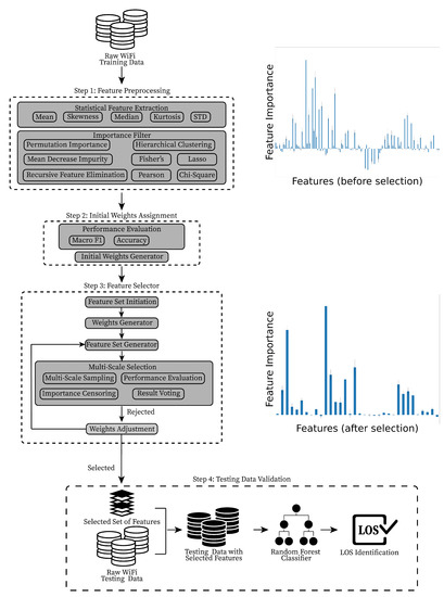
Figure 2.
The architecture of our proposed framework. As illustrated in the bar plot, our proposed framework greatly reduced the number of features while keeping the most informative ones.
- Step 1: A feature preprocessing method is proposed to extract the statistical features from raw WiFi training data. The mean, median, standard deviation, Kurtosis, and Skewness are calculated. Then, several Machine Learning feature selection models are used to analyze the importance of each feature and generate different sets of features.
- Step 2: Each feature set will be assigned an initial weight based on its macro F1 score and accuracy. These weights will be fed into the Feature Selector in the next step, and used for generating an initial set of features.
- Step 3: A multi-scale selection (MSS) method is used to reduce the weights of the uninformative features. The MSS method uses several scales of the datasets to select the features from different perspectives. In doing so, features that are important in both long-term time and short-term periods would be selected. The process is repeated until an optimal set of features is decided.
- Step 4: Using the selected set of features from the previous step, a LOS identifier (e.g., Random Forest Classifier) is employed to make LOS detections for the WiFi APs.
3.2. Problem Formulation
Without loss of generality, the test bed is evenly divided into grids where each cell represents a reference point. Please note that there is no overlapping reference point in training and testing data. A total of J grids is used as training reference point . K consecutive scans of raw WiFi RSS and RTT signal measures from T number of WiFi APs are collected at every point : and .
The LOS condition of each AP at the reference point is defined as , as follows:
where .
The raw training data are defined as , where and .
When the raw testing WiFi signal measures at are collected by the user, it will be preprocessed so only the features selected by the Feature Selector will remain. Then RFC identifies the LOS conditions of the AP. Finally, the LOS detection result is generated.
4. Feature Preprocessing and Feature Selection Algorithms
This section provides detailed descriptions of our proposed framework, including the feature preprocessing, initial weights assignment, feature selector and data validation.
4.1. Feature Preprocessing
As shown in Algorithm 1, during the Feature Preprocessing step, the statistics of the WiFi RSS and RTT are computed and filtered based on their importance and correlation to the LOS ground truth. Several traditional feature selection models are employed to analyze the importance of the features.
| Algorithm 1 Feature preprocessing and initial weights assignment |
|
4.1.1. Statistical Feature Extraction
Using the raw WiFi training data, the preprocessing step leverages a feature extraction method to generate the statistical features. Mean (), median (), standard deviation (), Skewness () and Kurtosis (), which were reported to be the most informative features for LOS identification [2], are computed from the WiFi RSS and RTT input data. For statistics calculation, the mean and central moment are defined as follows:
where indicates the RTT or RSS data collected at a specific reference point, K is the total number of data samples for statistics calculation, is the nth central moment. Based on the mean () and nth central moment , standard deviation (), Skewness () and Kurtosis () are computed as follows:
The raw training data will be replaced by a new statistical feature vector , , , , , , , , , .
4.1.2. Importance Filter
In this step, an importance filter is employed to remove the less important features from the previous feature preprocessing step. Several feature selection models are leveraged to analyze the importance and correlations of the features in to the ground truth label . Each model selects the top features based on their evaluation for the next step. The statistical features are ranked by their importance so that the least important features and those with the weakest correlation to the ground truth are removed.
We use the most popular feature selection models, namely Permutation Importance (PI), Hierarchical Clustering (HC), Fisher’s Score (Fisher), Recursive Feature Elimination (RFE), Least Absolute Shrinkage and Selection Operator (Lasso), Mean Decrease in Impurity (MDI), Pearson Correlation (Pearson) and Chi-squared (Chi). A short description of the models is as follows:
Permutation Importance (PI) The Permutation Importance model uses the mean decrease in accuracy of a chosen classifier as the evaluation metric to calculate the feature’s importance. To investigate the importance of each feature from the original feature set, PI randomly shuffles every feature during the iteration r. The shuffled feature set is then fed into the classifier for identification. The impact of the shuffled feature is illustrated by mean accuracy decrease . Thus, the correlation between the feature and the ground truth label could be evaluated which is also suitable for non-linear feature selection purposes [73]. The mean decrease accuracy importance of is calculated using both the average accuracy of shuffled data and the accuracy performance of the original feature set, as follows:
As shown in Figure 3, the importance of each feature in the proposed dataset is listed in their original order from left to right. Please note that features with negative MAD values are of the least importance for LOS detection.
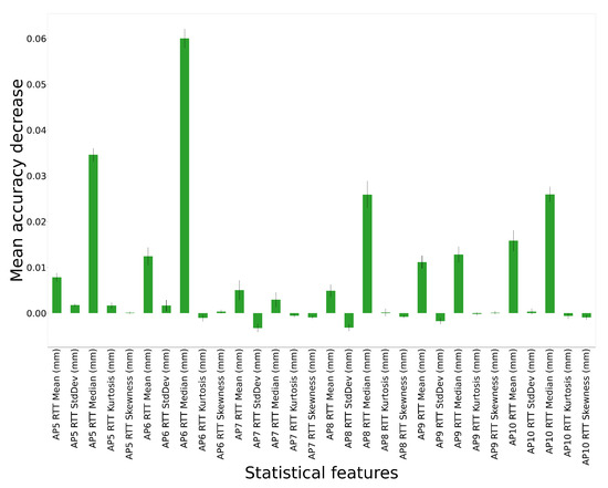
Figure 3.
A snapshot of some most important statistical features selected by the Permutation Importance (PI) model. The X-axis indicates different statistical features from the dataset. Negative mean accuracy values indicate that the corresponding features have the least correlation to the ground truth labels. We observe that AP #6 located in the middle of the testbed is the most informative AP for LOS identification.
We chose this model, as it was the underlying model to achieve more than 90% accuracy in breast cancer margins identification [74], and high accuracy in short-term electricity load forecasting [75].
Hierarchical Clustering (HC) Although the above permutation importance model already investigates the correlation between each feature and the output, some features may have similar importance when they are closely relevant. Therefore, redundant features still remain in the feature set after the selection by the PI model. To avoid the impact of duplicated information, Hierarchical Clustering (HC) is introduced.
To identify closely related features, HC groups all the features in separate clusters so that each cluster is clearly distinguishing from the rest. First, HC assigns every feature to a unique cluster. By leveraging Ward’s linkage function distance matrix converted from Spearman correlation matrix, HC investigates the similarity among the clusters. Then, the two most similar clusters are merged. By recursively repeating this process, the final set of feature clusters are decided where each cluster only contains features that are most similar to each other.
An example of the final clusters generated by HC is shown in Figure 4. Figure 5 demonstrates the correlations between every two features ().
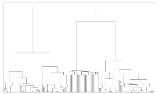
Figure 4.
The result from Hierarchical Clustering (HC). From the top node to the bottom, features are divided by their correlations to the others. Further separated features are less similar to each other. Please note that the order of the features listed is based on the result of HC.
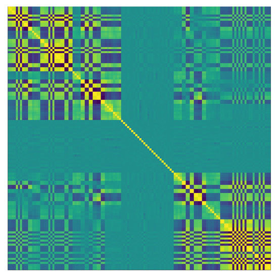
Figure 5.
The correlation between features from Hierarchical Clustering (HC). The X and Y axis represent the same set of features listed in the same order. Please note that this order is based on the result of HC. Lighter color indicates stronger correlation.
We employ this model, as it was reported to achieve high classification accuracy for daily electricity usage prediction with 97% less computational cost [76], and reached 99% accuracy of classification on non-iid (not independent and identically distributed) data [77].
Fisher’s Score Fisher’s score is one of the most popular filter methods among feature selection models. It evaluates the importance of the feature by computing the score between each feature and all the classes in the ground truth label. Then, the features are ranked to filter out the least important ones. The intuition of Fisher’s score is that the most informative features of a class should be more concentrated within the class while being further away from other classes. Fisher’s score is defined as:
where n represents the feature, l indicates the class in the label, is the number of data samples in the class, and are the mean and variance of the feature in class l, is the mean of the feature in all classes.
We employ the Fisher’s score, as it was the underlying feature selection method in other application domains with reported high accuracy (e.g., intrusion detection systems with 99% success rate [78], speech emotion recognition with 85% accuracy [79]).
Recursive Feature Elimination (RFE) The Recursive Feature Elimination model analyzes the importance of the feature by evaluating the change in the cost function. The intuition of RFE is such that removing an informative feature has a considerable impact on the cost function. Therefore, the larger and more rapid changes it causes to the cost function, the more important a feature is to the LOS identification. After removing a feature from the original set, the RFE model would calculate the changes to the cost function J immediately. Using Support Vector Machine (SVM) to assign the weights, RFE eliminates the features with the least importance iteratively. The changes in the cost function are defined as [80]:
where indicates the change in the weight of .
The importance of a feature is evaluated based on . The whole process is repeated until a feature set of the expected size is decided. For non-linear feature selection, the Gaussian kernel was proven to provide better results [81].
We employ RFE, as it was reported to achieve high accuracy with other application domains (e.g., fault diagnosis detection with an F1-measure of up to 0.95 [81]).
Least Absolute Shrinkage and Selection Operator (Lasso) Least Absolute Shrinkage and Selection Operator is an embedded feature selection model that gives a weight of 0 to the least important features. By leveraging L1 regularization (i.e., introducing L1-norm to the cost function), Lasso is able to select the best features in high-dimension datasets. The cost function in Lasso in defined as:
where is the number of data samples, is the label of the input data, is the feature set, is the slope term corresponding to each feature and is the penalty term indicating how severe the regularization is. In a set of closely correlated features, Lasso only selects one of them rather than adopting the whole combination.
We employ Lasso, as it was reported to achieve high accuracy with other application domains (e.g., crime prediction [82], tumor classification) with more than 81% accuracy [83].
Mean Decrease in Impurity (MDI) In contrast to the Permutation Importance, Mean Decrease in Impurity measures the feature importance by calculating the average decrease in Gini impurity [84]. In each node of a decision tree, every informative feature would help to reduce the Gini impurity. For a randomly selected variable, the Gini impurity indicates the probability of misidentification in this node, as follows:
where L is the number of classes to be identified in the ground truth label, is the probability of the data to be identified as class , t is a specific node in Random Forest, and are the child nodes of t, is the input to the t, and are data divided into and , respectively.
Therefore, the weighted average decrease in the impurity of each related node t would represent the importance of the corresponding feature [85]. The performance of MDI was investigated in [86]. It was observed that by leveraging features selected by MDI, an error rate as low as 4% was achieved.
Pearson correlation coefficient The Pearson correlation coefficient measures the linear correlation between each feature and the ground truth label to select the most important features. The covariance of the label and the feature set is leveraged by the Pearson correlation coefficient. The positive value of the covariance indicates a positive correlation between the feature and the ground-truth LOS conditions. Pearson correlation coefficient is defined as follows:
where E is the mathematical expectation, and are the input feature and the label, and are the mean values of and , and and are the standard deviation of and .
We employ the Pearson correlation coefficient, as it was reported to achieve high accuracy with other application domains (e.g., daily activity recognition [87] with more than 86% accuracy).
Chi-squared The Chi-squared model evaluates the importance of the features by calculating their correlations to the ground-truth labels . The Chi-squared score of each feature is calculated where N is the total number of statistical features in as:
where in our case is the observation results in LOS identification based on ground-truth label and WiFi signal features in , and represents the expected output of the identifications where and has no correlation at all. Since the Chi-squared score has an approximate Chi-squared () distribution in large-scale data, the higher the , the more important and relevant the feature is to the identification result.
We employ the Chi-squared model, as it was reported to achieve high accuracy with other application domains (e.g., Arabic text recognition [88] with 90.50% accuracy).
4.2. Initial Weights Assignment
With the above importance filter, the feature sets (where m indicates different selection models) were chosen by the feature selection models. However, the generated feature sets are not guaranteed with high identification accuracy and therefore, are not equally informative to the result. Thus, in this step, the selected statistical features , are evaluated and assigned with initial weights. The LOS identification performance of all feature sets are investigated by leveraging Random Forest Classifier (RFC) and cross-validation. The macro F1 score (the average F1 score of all classes) and the accuracy are used as the evaluation metrics, as follows:
where L represents the total classes in the ground-truth label, is the number of the true positive predicts, is the number of the false positive, and is the number of the false negative.
After obtaining the LOS identification performance evaluation, an evaluation vector is generated for each feature set based on the Macro F1 score and accuracy. Next, different initial weights are generated by the Initial Weights Generator based on all the evaluation vectors of the feature set . All selected features in the generated feature set is assigned with the same weight . If a feature is filtered out by the feature selection model, it is given the weight 0. The general weight of a statistical feature is defined as follows:
where is assigned with the weight of 0 when the corresponding is not selected by .
4.3. Feature Selector and Testing Data Validation
In this step, we propose the feature selector to validate the statistical features from the previous step.
4.3.1. Multi-Scale Selection (MSS)
To analyze the selected features in both long-time and short-time periods, a novel multi-scale selection method is proposed (see Figure 2). By using datasets of different sampling scales, MSS removes the features with the weakest correlation and decides on an optimal feature set with the minimum size as shown in the Algorithm 2. This step consists of four separate processes, namely multi-scale sampling, performance evaluation, importance censoring and result voting. A comprehensive description of these processes is given below.
| Algorithm 2 Feature selector with multi-scale selection. |
|
Multi-Scale sampling First, to investigate the feature performance on datasets, multi-scale sampling is adopted to generate datasets with different sampling sizes. For our dataset, a maximum of 120 scans of WiFi measures were recorded in each reference point. Thus, we evaluate different sampling sizes from five scans (i.e., short-term sudden change) to 120 scans (i.e., long-term measure). As illustrated in Section 5.4, adopting different sampling sizes has a clear impact on LOS identification.
Performance evaluation Next, the same evaluation methods in Section 4.2 are employed to analyze the feature performance on multi-scale datasets. The evaluation vectors of the feature set on different datasets indicate the importance of each feature for LOS detection. After a new feature set is generated based on the updated weights, RFC is used to perform LOS identification.
Importance censoring Since the features are re-sampled according to different sampling sizes, the hidden patterns that indicate the LOS condition change accordingly. Thus, we use the feature selection models from the above importance filter to evaluate the relevance of the features from different perspectives.
Result voting After obtaining the RFC performance and importances generated by the above selection models, the features with the strongest correlations to multi-scale LOS identification are selected. Result voting is leveraged to rank the statistical features. With both empirical performance and theoretical evaluations, the most informative and relevant statistical features to LOS detections in the current set are decided. Features with higher voting scores on multi-scale datasets receive increments in their corresponding weights.
4.3.2. Final Feature Set and Testing Data Validation
After the weights update in the previous step, the features with lower weights (those with uninformative information for LOS identification) are rejected, the weights generator and feature set generator select a new feature set based on these updated weights . The new feature set will be fed into MSS for further iterations. When the final set of features remains unchanged, this set will be used for data validation.
In the testing phase, the WiFi signal measures collected from the new reference points are preprocessed. Statistics of WiFi RSS and RTT measurements are extracted to form a statistical testing dataset . By only keeping the features selected by the final feature set from MSS, a new dataset containing only the most informative features is generated.
5. Experimental Setup and Empirical Results
In this section, a comprehensive description of the proposed dataset is introduced. Then, we evaluate the proposed framework on this dataset.
5.1. Test Bed and the Proposed Dataset
Although identifying LOS conditions of APs is of significant value for WiFi indoor positioning systems, to the best of our knowledge, there is no publicly available dataset that contains both the WiFi RTT, RSS signal measures and the LOS condition of the reference points. Furthermore, there is no public WiFi positioning dataset that contains multiple samples of both RTT and RSS per reference points, that are needed for statistical analysis of the signal measures. Therefore, it is necessary to have a public dataset that fulfills the above criteria for further WiFi indoor positioning research. This motivates us to collect and publish our own large-scale real-world WiFi RSS and RTT datasets for the community.
We chose the entire fifth floor of a campus building as the testbed (see Figure 6). The space was filled with furniture and a noisy background with plenty of electromagnetic signal transmitters. The indoor interior includes long narrow corridors, big meeting rooms, small office rooms, and large open space. The variety of LOS and NLOS scenarios in this testbed makes it suitable for testing our proposed LOS identification algorithms.
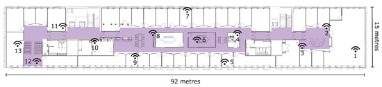
Figure 6.
The layout of the building floor. The icons show the locations of the WiFi APs. Measurements were taken in the shaded area. The numbers next to the icons indicate the IDs of the Access points.
For WiFi signal measurements, an LG G8X ThinQ smartphone and 13 RTT-enabled Google APs were used. The APs were placed in the exact same locations as the university’s regular APs. Using measuring tapes and ground markers, the ground-truth coordinates of each reference point were carefully recorded and validated by human testers. In addition, the LOS conditions of all APs from each reference point were manually collected and verified. The detailed information of the proposed dataset is listed in Table 2. The dataset is made public at https://github.com/Fx386483710/WiFi-RTT-RSS-dataset (accessed on 10 April 2020).
Table 2.
Summary of our dataset.
A snapshot of the WiFi RSS and RTT measurements of our dataset is shown in Table 3. The values in columns ‘X’ and ‘Y’ are the ground-truth coordinates of the reference point. Columns ‘AP1’ to ‘AP13’ show the WiFi RSS and RTT from all APs at such reference point. The value of −200 dBm indicates that the corresponding AP is not visible from the current position. Similarly, the value of 100,000 mm demonstrates that no WiFi RTT signal is received from the corresponding AP. Column ‘LOS APs’ shows which APs the reference point has a direct LOS path to. In our dataset, 120 scans (i.e., approximately 40 s) of data samples are recorded at each reference point, which provides sufficient information for further research. Please note that the reference points in the training and testing dataset do not overlap. A desktop PC equipped with an Intel i9-12900k @ 4.90 GHz CPU and 32 GB DDR4 4000 MHz memory was used to analyze the results.
Table 3.
A Snapshot of the proposed WiFi dataset.
5.2. The Impact of NLOS Scenarios in Indoor Positioning
In NLOS scenarios, the WiFi signals are interfered, causing a negative impact on the signal measurements. In the indoor environments, the signals are easily attenuated by thick concrete walls, humans and furniture, making it challenging for indoor positioning. As illustrated in Figure 7, the WiFi RSS measurements were not stable over time. Most importantly, we observed that even though strong signal measures of −60 dBm were received, the same NLOS WiFi AP could not be reached at some point.
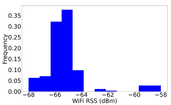
Figure 7.
A histogram of the WiFi RSS signal measurement from the dataset proposed in Section 5.1. We observed that the RSS measures were unstable and easily attenuated during long observation period.
To have a deeper understanding of the real-world impact of NLOS conditions, we recorded the WiFi RSS and RTT signal measurements under two scenarios: LOS where there was a clear path between the AP and the smartphone, and NLOS where there was a human body in-between. The smartphone was placed 3 m away from the AP. We observed in Figure 8, Figure 9 and Figure 10 that under the NLOS scenario, both signal measures were unstable. For WiFi RSS, the recorded measurement values decreased drastically from −54 dBm to −80 dBm. Additionally, the distribution of the WiFi RSS became wider. However, we observed that although the RTT measures became larger, its distribution was less affected than RSS under the NLOS scenario. There were occasional outliers of up to 4 m (from the ground-truth of 3 m). Under LOS conditions, both WiFi RSS and RTT signals were stable and exhibited a small distribution. Therefore, with correct calibration, the RTT measures could locate the user with good accuracy by trilateration. It was also observed in the CDF curve that the variance of the LOS RTT measures stayed within 0.5 m while NLOS had a variance of up to 3.5 m. Therefore, successfully identifying the LOS conditions of each AP would help improving the indoor positioning accuracy.
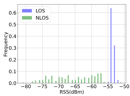
Figure 8.
The WiFi RSS signal measure under different scenarios. A smartphone was placed 3 m away from the access point. We observed that in NLOS experiment where the signal was blocked by human body, the RSS measurement became unstable and reduced drastically due to the NLOS condition.
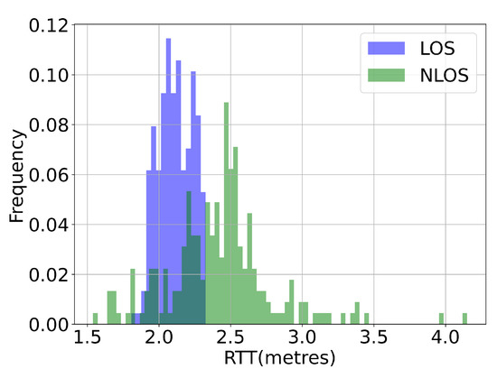
Figure 9.
The WiFi RTT signal measure under different scenarios. A smartphone was placed 3 m away from the access point. We observed that in human NLOS experiment where the signal was blocked by human body, the RTT measurement became larger, more unreliable and further away from the ground truth distance measure.
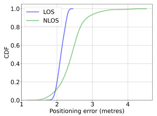
Figure 10.
The CDF curves of WiFi RTT signal measure under different scenarios. A smartphone was placed 3 m away from the access point. We observed that in human NLOS experiment where the signal was blocked by human body, the minimum error of the RTT measurement increased and the maximum error grew larger as well. WiFi RTT became more unreliable under NLOS scenarios.
To investigate the impact of a dynamic indoor environment on the signal measures, we collected both WiFi RSS and RTT measures under three scenarios: LOS, NLOS and corridor LOS. The smartphone was moving away from the AP while recording WiFi data. To create a common NLOS condition, the AP was placed on the other side of a thick concrete wall. In the corridor experiment, although the AP had a clear LOS path to the smartphone in a narrow long corridor, the WiFi signals struggled under the heavy reflections created by the walls. To analyze the correlation between the WiFi signals measurements and the true distance, the RSS and RTT values were normalized. As shown in Figure 11, Figure 12 and Figure 13, in an ideal LOS experiment, the RSS measures (in green color) had much smaller variance under LOS conditions. However, the RTT measure (in orange color) showed its robustness in the NLOS scenario by producing a similar level of variance as the RSS measures. In the corridor experiment, it was observed that the RSS measures were greatly attenuated by the interior, where locations up to 9 m away from the AP had similar RSS. On the contrary, the RTT measure showed clear correlations to the true distance with some minor offsets. We concluded that the RTT measures were more robust and reliable in more complex environments and the RSS measures were more sensitive to the interior changes.
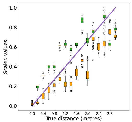
Figure 11.
The comparison of the WiFi RSS and RTT measurements as a function of the true distance in LOS scenario. The RSS (as shown in green color) and RTT (as shown in orange color) values were normalized. We observed that under LOS conditions, RSS measures were more resilient.
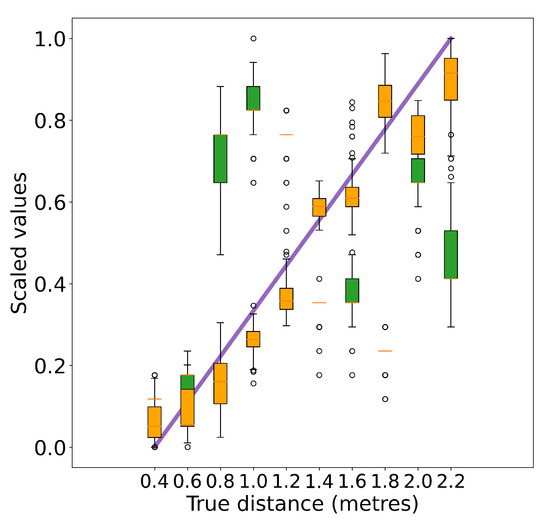
Figure 12.
The comparison of the WiFi RSS and RTT measurements as a function of the true distance in a NLOS scenario. The WiFi signal was blocked by a thick wall. The RSS (as shown in green color) and RTT (as shown in orange color) values were scaled between 0 and 1. We observed that under NLOS conditions, RSS and RTT measures had similar variance.
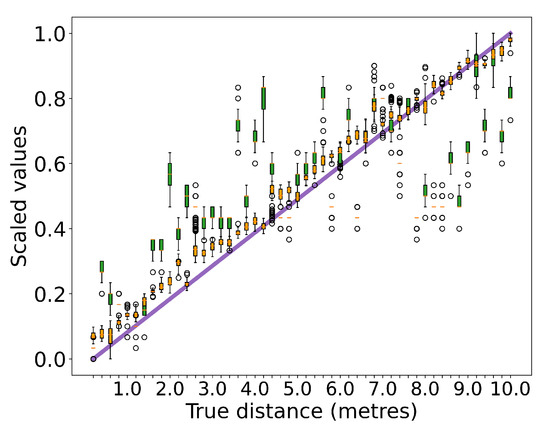
Figure 13.
The comparison of WiFi RSS and RTT measurements as a function of the true distance in a long narrow corridor. The WiFi signal suffered from severe reflections and attenuations. The RSS (as shown in green color) and RTT (as shown in orange color) values were normalized. We observed that in complex indoor spaces, the RSS produced large variance even with clear LOS path to the AP. The RSS measurements were unpredictable with similar values up to 9 m away. In contrast, the RTT measures were more stable and had a clear positive correlation to the true distance.
As shown in Figure 14 and Figure 15, when using only raw statistical features from all LOS APs, the positioning error was 1.18 m. However, after introducing NLOS APs, the error increased to 1.41 m. When only NLOS signals are included, the positioning error went up to 1.65 m. In addition, the largest RMSE produced by NLOS features was up to 7 m. We observed that using LOS WiFi signals could greatly improve the positioning accuracy by up to 29%. Please note that the results were based on raw statistical features. The above empirical results indicate that identifying the LOS conditions of the APs is of great importance.
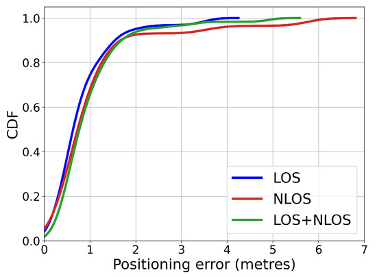
Figure 14.
The CDF result of WiFi fingerprinting using the signal measures from only LOS APs, NLOS APs, and all the APs. Please note that all statistical features from the corresponding APs were leveraged. Introducing NLOS signal measures greatly reduced the performance accuracy. The largest positioning error was up to 7 m.
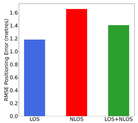
Figure 15.
The RMSE result of indoor positioning WiFi signal measures from only LOS APs, NLOS APs, and all the APs. Please note that all statistical features from the corresponding APs were leveraged. Using only raw statistical features from LOS APs improved the positioning accuracy by up to 29 % compared to only using NLOS signals.
5.3. The Importance of Feature Selection
In LOS identification, higher accuracy is not guaranteed with more data. The WiFi signals are unstable and may introduce more errors into the positioning result. To assess the impact of introducing raw WiFi statistical features, we used the random forest classifier to perform LOS detection. WiFi AP6, AP8 and AP12 were chosen as examples for individual LOS detection because they had the most LOS paths to the RPs. The positions of the three APs are as shown in Figure 6. The performance of using unmodified statistical features is illustrated in Figure 16 and Table 4. We observed that using all the raw features from the corresponding AP does not guarantee better accuracy. The WiFi signals from AP12 contained more noisy information for the classifier. On the contrary, using features from all APs failed in LOS detection of AP6. We observed that to achieve robust LOS detection results, selecting the most meaningful features is of great importance.
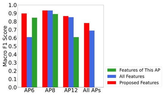
Figure 16.
The performance of all APs and individual AP LOS identification using different sets of features. Please note that features included are all statistical features introduced in Section 4.1.1.
Table 4.
The Macro F1 score performance of all APs and individual AP LOS identification using different sets of features.
5.4. Sampling Size
The novel idea of developing the multi-scale selection method is to analyze the importance of the statistical features from both macroscopical and microscopical perspectives. The signal patterns indicating the LOS condition of each AP were investigated in both long-term and short-term time periods. Therefore, stable measurements and sudden changes were included in identifying LOS conditions. As demonstrated in Figure 17, statistical features from datasets of different sampling sizes provide distinguishing information. For features from 120 to scan data, only the mean value of all RTT measurements was kept. The outliers and fluctuating measurements were removed during the feature extraction phase. In contrast, the 5-scan dataset still recorded the abnormal RTT measures at the reference point which implied a higher possibility of the NLOS condition of the AP.
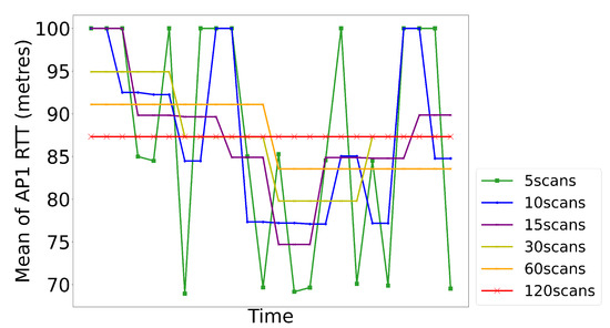
Figure 17.
The mean value of AP1’s RTT measures with different sampling sizes at a RP. The value of 100 indicates that there is no WiFi signal at this RP. Datasets of different sample sizes contain signal patterns of different time period.
To illustrate the significance of the MSS method, LOS identification performance was evaluated on multi-scale datasets. Datasets of different sampling sizes (i.e., 5, 10, 15, 30, 60, 120) were generated by MSS. For the dataset with a minimum of five scans, every 1.5 s WiFi signal measures were used to form the statistical features. AP6, AP8, and AP12 were chosen for individual AP LOS detection because they had the most LOS paths to the RPs. The positions of the three APs are as shown in Figure 6. The performance results of LOS identifications using multi-scale datasets are shown in Figure 18 and Table 5. In the proposed framework, we focus on the LOS conditions of both individual AP and all APs at the same time. As illustrated in the results, using smaller sampling sizes had an improvement in identifying the LOS of certain APs. However, such influence became negative when predicting the conditions of all APs at the same time. We observed that the features selected by the proposed MSS method had a great improvement in the performance of both individual and all-AP LOS predictions.
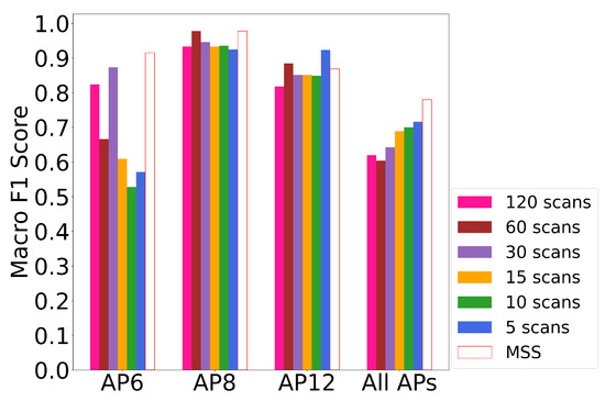
Figure 18.
The performance of all APs and individual AP LOS identification using datasets of different sampling sizes, compared to MSS. Statistical features of all APs were used except for MSS where only selected features were used. Features selected by MSS are more informative than features from single sample size dataset.
Table 5.
The Macro F1 score performance of all APs and individual AP LOS identification using datasets of different sampling sizes, compared to MSS.
5.5. The Performance of the Proposed Framework
Since using all statistical features had a poor performance in LOS detections, feature selection algorithms were introduced to address the problem. By leveraging feature selection models, features with redundant information were removed, while noisy features were marked for further improvement.
For performance evaluation of the proposed framework, WiFi RSS and RTT datasets containing the ground-truth coordinates and LOS conditions are needed. However, currently, there is no publicly available dataset that meets this requirement. Therefore, to validate the LOS identification accuracy and assess the transferability and generalization of our proposed framework, a large-scale real-world dataset was proposed as introduced in Section 5.1. By evaluating the performance on both individual AP and all APs LOS identification, we illustrate the transferability and generalization of the proposed framework.
Several state-of-the-art feature selection algorithms were used for comparison. In addition to popular feature selection models (i.e., PI, HC, Fisher, RFE, Lasso, MDI, Pearson, and Chi) as introduced in Section 4.1.2, algorithms proposed by previous works were included. The model proposed by [69] used the mean RSS measurement and other statistical features (e.g., mean, quantile deviation, number of outliers) extracted from RTT measures. In the paper by Dong et al. [69], different manually selected combinations of the features were tested. S-F [71] leveraged the mean, standard deviation, Skewness, and Kurtosis of both WiFi RTT and RSS measures. The features set (represented as ) selected by [68] contained standard deviations of both RTT and RSS. Consisting only of raw RSS and RTT measures, the set [89] identified APs sending both large RTT measures and low RSS measures as NLOS. In the feature set chosen by [66], mean and variance of the RSS were leveraged. The system proposed [70] used standard deviation, skewness, kurtosis, hyper-skewness, and peak probability as the neural network input for WiFi channel LOS identifications, represented by . The 10-scans dataset was used because it was the most indicative based on the above empirical results. Macro F1 score and weighted F1 score were used as evaluation metrics. Macro F1 score focused on valuing all APs equally while the weighted F1 score balanced the disparity among the classes.
The identification of LOS conditions of all APs was performed based on different feature selection models. The performance of each algorithm is illustrated in Figure 19 and Table 6. We observed that the feature set selected by the proposed framework improved the LOS identification results greatly. In macro F1 score, the proposed framework achieved up to 126% improvement compared to previous work and up to 29% compared to popular feature selection models. For weighted macro F1 score, the proposed framework achieved up to 81% improvement compared to previous work and up to 16% compared to popular feature selection models. Our proposed framework also used fewer features, with only 34 out of 130 features. The number of features used by Pearson and Fisher models was more than 110 and 90, respectively. The result demonstrated that further analysis of the feature importance in the multi-scale datasets provided higher accuracy. As shown in Figure 20, the misclassifications happened mostly in reference points that were located in cornered areas. We observed from Figure 20 that stable and strong WiFi connections would provide more reliable LOS identification.
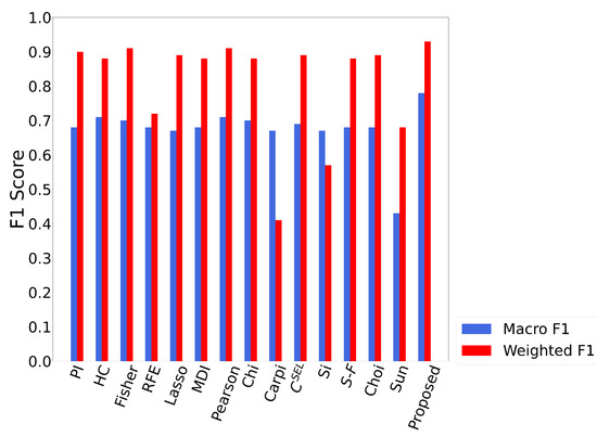
Figure 19.
The performance of different sets of features in all APs LOS identification. Our proposed MSS is up to 28.8% better than popular feature selection models and up to 14.5% better than state-of-the-art WiFi LOS identification algorithms.
Table 6.
Comparison of the LOS identification performance of previous state-of-the-art.
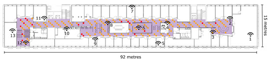
Figure 20.
The RPs where the system makes misidentification. The orange dots indicate the RPs of testing data while the red indicate the misidentifications. Most misidentifications took place in areas surrounded by complicated interior changes.
Furthermore, the proposed framework was evaluated on its individual AP LOS detection. As shown in Figure 21, APs that had LOS path to any RPs were included in the evaluation. AP6, AP8 and AP12 had LOS paths to the most RPs while AP7 and AP10 only had LOS paths to 8 RPs and 4 RPs, respectively. It was observed that the proposed framework provided promising performance in LOS identifications for individual APs even with a LOS path to a few RPs.
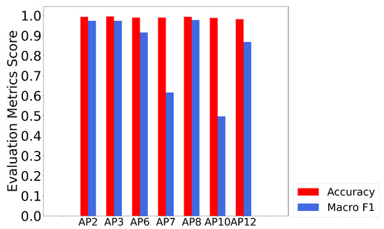
Figure 21.
The performance of the individual AP identification. APs which do not have LOS path to any RP are not included. Please note that only 8 and 4 RPs have LOS path to AP7 and AP10, respectively. MSS selected features achieve more than 0.5 F1 score performance even in APs with insufficient data.
6. Discussion
We compared our proposed framework with several feature selection models and LOS identification algorithms from previous works, in empirical settings. We observed that our framework increased the macro F1 score and weighed F1 score by up to 15.3% and 28.8%, respectively. Most importantly, our framework used fewer features compared to existing state-of-the-art models.
The major improvement in our feature selection progress is that instead of enumerating different combinations of features manually (as adopted by previous works), the proposed framework automatically selects the best set of features. The final selection is only based on the input features and ground-truth label which guarantees the framework’s transferability to high-dimensional data of other signal measurements. For instance, WiFi RTT measurements collected from ESP32 system using Chronos software [54] can be used directly as the input to the proposed framework with no restrictions. The framework would only investigate the correlations between the input features and the ground-truth label and select the best set of features accordingly. The proposed MSS method investigates the feature importance in multiple sampling scales so that the final set of features is informative from both macroscopical and microscopical perspectives.
To validate the generalization of the framework, a novel dataset was collected. To the best of our knowledge, there is no existing WiFi dataset that contains detailed WiFi RSS, RTT signal measurements, ground-truth coordinates of the reference points, and LOS conditions of all APs to each reference point. The contributions of the dataset to the research field are as follows:
- The dataset was collected in a campus floor. Each AP was surrounded by complex interiors and in different LOS/NLOS conditions.
- The testbed of 92 × 15 m2 was evenly divided into 0.6 × 0.6 m grids which served as reference points. Each grid was carefully labeled with ground-truth coordinates by two human surveyors. Reference points for training and testing are not overlapping.
- At each reference point, more than 120 scans of both WiFi RTT and RSS signal measurements were collected. During collection, the influence of the human body was taken into consideration.
- Each data sample was meticulously labeled with LOS conditions of all the APs in the testbed.
- With more than 77,000 samples, the dataset provides good coverage for the evaluation of any WiFi RSS-based, RTT-based or hybrid indoor positioning systems. The real-world indoor environment guarantees the generalization of the proposed framework.
7. Conclusions and Future Work
In this article, a novel feature selection framework for LOS identification of WiFi APs was introduced. Our proposed framework efficiently selects the most optimal set of informative features for identifying WiFi LOS scenarios. Different from previous state-of-the-art techniques where features were selected manually, our framework automatically investigates the importance of each feature on multi-scale datasets.
In the preprocessing stage, statistics of the input WiFi measurements were computed and fed into the importance filter. Several popular feature selection models were used in the importance filter to decide their own feature set based on different algorithms. Then, in the initial weight assignment step, the statistical features chosen by feature selection models were assigned with initial weights based on their macro F1 score and accuracy in LOS identification. Based on the empirical experience, RFC was used as the LOS identifier in our framework. Next, to validate the selected features from both macroscopical and microscopical perspectives, multi-sampling datasets are introduced in the feature selector. Based on the performance of the selected feature set, importance censoring and result voting were leveraged to adjust the weights of the features recursively. In the testing stage, the proposed framework extracts the same features from the testing data selected by the feature selector.
For evaluation of the framework, a dataset was collected in a large-scale real-world indoor environment. More than 120 scans of data samples were recorded and carefully labeled by two human surveyors. Since each AP was surrounded by complex interiors, the generalization of the proposed LOS identification algorithm could be validated. To investigate the improvement brought by feature selection, we compare the proposed framework with raw statistical features on individual AP and all APs identification. It was observed that using selected features by the proposed work improved the macro F1 score by up to 50%. We observed that using only 3 s data, the proposed framework provided promising LOS detection accuracy which is up to 93% for all APs at the same time and 98% for individual AP.
For future work, we may improve the combinations and selections of different feature selection models used in the importance filter (see Section 4.1.2) which may reduce the time cost and enhance the efficiency of the proposed framework. Furthermore, sliding windows in different sampling scales may be considered for implementation in multi-scale selection as introduced in Section 4.3.1. The sampling method leveraged in the proposed framework was not sensitive to different segmentations of a long consecutive data record. Using sliding window may help the framework to select better features for LOS identification. The proposed framework focuses on investigating the importance of the feature to the ground truth label. It takes the features for classification or regression systems as the input, and outputs a selection of the most informative features. Therefore, it is not restricted to WiFi RSS and RTT signal measurements. Due to the great transferability of the proposed framework, it could be implemented to reduce high-dimensional data collected from other signal measurements, such as CSI, CIR, and UWB.
Author Contributions
Conceptualization, X.F., K.A.N. and Z.L.; methodology, X.F.; software, X.F. and K.A.N.; validation, X.F., K.A.N. and Z.L.; formal analysis, X.F., K.A.N. and Z.L.; investigation, X.F. and K.A.N.; resources, X.F., K.A.N. and Z.L.; data curation, X.F. and K.A.N.; writing—original draft preparation, X.F.; writing—review and editing, K.A.N. and Z.L; visualization, X.F.; supervision, K.A.N. and Z.L.; project administration, K.A.N. and Z.L.; funding acquisition, K.A.N. All authors have read and agreed to the published version of the manuscript.
Funding
This research was funded by the University of Brighton.
Data Availability Statement
Publicly available datasets were analyzed in this study. This data can be found here: https://github.com/Fx386483710/WiFi-RTT-RSS-dataset.
Conflicts of Interest
The authors declare no conflict of interest.
References
- Nguyen, K.A.; Luo, Z.; Li, G.; Watkins, C. A review of smartphones-based indoor positioning: Challenges and applications. IET Cyber-Syst. Robot. 2021, 3, 1–30. [Google Scholar] [CrossRef]
- Huang, C.; He, R.; Ai, B.; Molisch, A.F.; Lau, B.K.; Haneda, K.; Liu, B.; Wang, C.X.; Yang, M.; Oestges, C.; et al. Artificial intelligence enabled radio propagation for communications—Part II: Scenario identification and channel modeling. IEEE Trans. Antennas Propag. 2022, 70, 3955–3969. [Google Scholar] [CrossRef]
- Liu, F.; Liu, J.; Yin, Y.; Wang, W.; Hu, D.; Chen, P.; Niu, Q. Survey on WiFi-based indoor positioning techniques. IET Commun. 2020, 14, 1372–1383. [Google Scholar] [CrossRef]
- Nguyen, K.A.; Luo, Z. On assessing the positioning accuracy of Google Tango in challenging indoor environments. In Proceedings of the 2017 International Conference on Indoor Positioning and Indoor Navigation (IPIN), Sapporo, Japan, 18–21 September 2021; IEEE: Piscataway, NJ, USA, 2017; pp. 1–8. [Google Scholar]
- Feng, X.; Nguyen, K.A.; Luo, Z. An analysis of the properties and the performance of WiFi RTT for indoor positioning in non-line-of-sight environments. In Proceedings of the 17th International Conference on Location Based Services, Munich, Germany, 12–14 September 2022. [Google Scholar]
- Nie, Z.; Liu, F.; Gao, Y. Real-time precise point positioning with a low-cost dual-frequency GNSS device. Gps Solut. 2020, 24, 9. [Google Scholar] [CrossRef]
- Marra, A.D.; Becker, H.; Axhausen, K.W.; Corman, F. Developing a passive GPS tracking system to study long-term travel behavior. Transp. Res. Part C Emerg. Technol. 2019, 104, 348–368. [Google Scholar] [CrossRef]
- Zein, Y.; Darwiche, M.; Mokhiamar, O. GPS tracking system for autonomous vehicles. Alex. Eng. J. 2018, 57, 3127–3137. [Google Scholar] [CrossRef]
- Zhang, E.; Masoud, N. Increasing GPS localization accuracy with reinforcement learning. IEEE Trans. Intell. Transp. Syst. 2020, 22, 2615–2626. [Google Scholar] [CrossRef]
- Gondelach, D.J.; Linares, R. Real-time thermospheric density estimation via radar and GPS tracking data assimilation. Space Weather 2021, 19, e2020SW002620. [Google Scholar] [CrossRef]
- Xu, B.; Jia, Q.; Hsu, L.T. Vector tracking loop-based GNSS NLOS detection and correction: Algorithm design and performance analysis. IEEE Trans. Instrum. Meas. 2019, 69, 4604–4619. [Google Scholar] [CrossRef]
- Wen, F.; Wymeersch, H.; Peng, B.; Tay, W.P.; So, H.C.; Yang, D. A survey on 5G massive MIMO localization. Digit. Signal Process. 2019, 94, 21–28. [Google Scholar] [CrossRef]
- He, J.; Wymeersch, H.; Kong, L.; Silvén, O.; Juntti, M. Large intelligent surface for positioning in millimeter wave MIMO systems. In Proceedings of the 2020 IEEE 91st Vehicular Technology Conference (VTC2020-Spring), Virtual Event, 25–28 May 2020; IEEE: Piscataway, NJ, USA, 2020; pp. 1–5. [Google Scholar]
- De Bast, S.; Guevara, A.P.; Pollin, S. CSI-based positioning in massive MIMO systems using convolutional neural networks. In Proceedings of the 2020 IEEE 91st Vehicular Technology Conference (VTC2020-Spring), Virtual Event, 25–28 May 2020; IEEE: Piscataway, NJ, USA, 2020; pp. 1–5. [Google Scholar]
- Lin, Y.; Jin, S.; Matthaiou, M.; You, X. Channel estimation and user localization for IRS-assisted MIMO-OFDM systems. IEEE Trans. Wirel. Commun. 2021, 21, 2320–2335. [Google Scholar] [CrossRef]
- Ma, J.; Zhang, S.; Li, H.; Gao, F.; Jin, S. Sparse Bayesian learning for the time-varying massive MIMO channels: Acquisition and tracking. IEEE Trans. Commun. 2018, 67, 1925–1938. [Google Scholar] [CrossRef]
- Zhang, J.; Salmi, J.; Lohan, E.S. Analysis of kurtosis-based LOS/NLOS identification using indoor MIMO channel measurement. IEEE Trans. Veh. Technol. 2013, 62, 2871–2874. [Google Scholar] [CrossRef]
- Chen, J.; Yin, X.; Cai, X.; Wang, S. Measurement-based massive MIMO channel modeling for outdoor LoS and NLoS environments. IEEE Access 2017, 5, 2126–2140. [Google Scholar] [CrossRef]
- Huang, C.; Molisch, A.F.; Wang, R.; Tang, P.; He, R.; Zhong, Z. Angular information-based NLOS/LOS identification for vehicle to vehicle MIMO system. In Proceedings of the 2019 IEEE International Conference on Communications Workshops (ICC Workshops), Shanghai, China, 22–24 May 2019; IEEE: Piscataway, NJ, USA, 2019; pp. 1–6. [Google Scholar]
- Zhang, Q.; Yang, H.H.; Quek, T.Q.; Lee, J. Heterogeneous cellular networks with LoS and NLoS transmissions—The role of massive MIMO and small cells. IEEE Trans. Wirel. Commun. 2017, 16, 7996–8010. [Google Scholar] [CrossRef]
- Zeng, T.; Chang, Y.; Zhang, Q.; Hu, M.; Li, J. CNN-based LOS/NLOS identification in 3-D massive MIMO systems. IEEE Commun. Lett. 2018, 22, 2491–2494. [Google Scholar] [CrossRef]
- Li, J.; Chang, Y.; Zeng, T.; Xiong, Y. Channel correlation based identification of LOS and NLOS in 3D massive MIMO systems. In Proceedings of the 2019 IEEE Wireless Communications and Networking Conference (WCNC), Marrakesh, Morocco, 15–18 April 2019; IEEE: Piscataway, NJ, USA, 2019; pp. 1–6. [Google Scholar]
- Ridolfi, M.; Kaya, A.; Berkvens, R.; Weyn, M.; Joseph, W.; Poorter, E.D. Self-calibration and collaborative localization for uwb positioning systems: A survey and future research directions. ACM Comput. Surv. (CSUR) 2021, 54, 1–27. [Google Scholar] [CrossRef]
- Poulose, A.; Han, D.S. UWB indoor localization using deep learning LSTM networks. Appl. Sci. 2020, 10, 6290. [Google Scholar] [CrossRef]
- Yu, K.; Wen, K.; Li, Y.; Zhang, S.; Zhang, K. A novel NLOS mitigation algorithm for UWB localization in harsh indoor environments. IEEE Trans. Veh. Technol. 2018, 68, 686–699. [Google Scholar] [CrossRef]
- Macoir, N.; Bauwens, J.; Jooris, B.; Van Herbruggen, B.; Rossey, J.; Hoebeke, J.; De Poorter, E. Uwb localization with battery-powered wireless backbone for drone-based inventory management. Sensors 2019, 19, 467. [Google Scholar] [CrossRef]
- Poulose, A.; Emeršič, Ž.; Eyobu, O.S.; Han, D.S. An accurate indoor user position estimator for multiple anchor uwb localization. In Proceedings of the 2020 International Conference on Information and Communication Technology Convergence (ICTC), Jeju Island, Republic of Korea, 21–23 October 2020; IEEE: Piscataway, NJ, USA, 2020; pp. 478–482. [Google Scholar]
- Musa, A.; Nugraha, G.D.; Han, H.; Choi, D.; Seo, S.; Kim, J. A decision tree-based NLOS detection method for the UWB indoor location tracking accuracy improvement. Int. J. Commun. Syst. 2019, 32, e3997. [Google Scholar] [CrossRef]
- Barral, V.; Escudero, C.J.; García-Naya, J.A.; Maneiro-Catoira, R. NLOS identification and mitigation using low-cost UWB devices. Sensors 2019, 19, 3464. [Google Scholar] [CrossRef]
- Park, J.; Nam, S.; Choi, H.; Ko, Y.; Ko, Y.B. Improving deep learning-based UWB LOS/NLOS identification with transfer learning: An empirical approach. Electronics 2020, 9, 1714. [Google Scholar] [CrossRef]
- Hajiakhondi-Meybodi, Z.; Mohammadi, A.; Hou, M.; Plataniotis, K.N. DQLEL: Deep Q-Learning for Energy-Optimized LoS/NLoS UWB Node Selection. IEEE Trans. Signal Process. 2022, 70, 2532–2547. [Google Scholar] [CrossRef]
- Cui, Z.; Gao, Y.; Hu, J.; Tian, S.; Cheng, J. LOS/NLOS identification for indoor UWB positioning based on Morlet wavelet transform and convolutional neural networks. IEEE Commun. Lett. 2020, 25, 879–882. [Google Scholar] [CrossRef]
- Li, H.; Zeng, X.; Li, Y.; Zhou, S.; Wang, J. Convolutional neural networks based indoor Wi-Fi localization with a novel kind of CSI images. China Commun. 2019, 16, 250–260. [Google Scholar] [CrossRef]
- Dang, X.; Tang, X.; Hao, Z.; Ren, J. Discrete Hopfield neural network based indoor Wi-Fi localization using CSI. EURASIP J. Wirel. Commun. Netw. 2020, 2020, 1–16. [Google Scholar] [CrossRef]
- Wang, X.; Wang, X.; Mao, S. Deep convolutional neural networks for indoor localization with CSI images. IEEE Trans. Netw. Sci. Eng. 2018, 7, 316–327. [Google Scholar] [CrossRef]
- Dang, X.; Tang, X.; Hao, Z.; Liu, Y. A device-free indoor localization method using CSI with Wi-Fi signals. Sensors 2019, 19, 3233. [Google Scholar] [CrossRef] [PubMed]
- Tong, X.; Wan, Y.; Li, Q.; Tian, X.; Wang, X. CSI fingerprinting localization with low human efforts. IEEE/ACM Trans. Netw. 2020, 29, 372–385. [Google Scholar] [CrossRef]
- Feng, X.; Nguyen, K.A.; Luo, Z. A survey of deep learning approaches for WiFi-based indoor positioning. J. Inf. Telecommun. 2022, 6, 163–216. [Google Scholar] [CrossRef]
- Li, Z.; Tian, Z.; Zhou, M.; Zhang, Z.; Jin, Y. Awareness of line-of-sight propagation for indoor localization using Hopkins statistic. IEEE Sen. J. 2018, 18, 3864–3874. [Google Scholar] [CrossRef]
- Zhou, Z.; Yang, Z.; Wu, C.; Sun, W.; Liu, Y. LiFi: Line-of-sight identification with WiFi. In Proceedings of the IEEE INFOCOM 2014-IEEE Conference on Computer Communications, Toronto, ON, Canada, 27 April–2 May 2014; IEEE: Piscataway, NJ, USA, 2014; pp. 2688–2696. [Google Scholar]
- Wu, C.; Yang, Z.; Zhou, Z.; Qian, K.; Liu, Y.; Liu, M. PhaseU: Real-time LOS identification with WiFi. In Proceedings of the 2015 IEEE Conference on Computer Communications (INFOCOM), Hong Kong, China, 26 April–1 May 2015; IEEE: Piscataway, NJ, USA, 2015; pp. 2038–2046. [Google Scholar]
- Zhou, Z.; Yang, Z.; Wu, C.; Shangguan, L.; Cai, H.; Liu, Y.; Ni, L.M. WiFi-based indoor line-of-sight identification. IEEE Trans. Wirel. Commun. 2015, 14, 6125–6136. [Google Scholar] [CrossRef]
- Chang, T.; Jiang, S.; Sun, Y.; Jia, A.; Wang, W. Multi-bandwidth NLOS Identification Based on Deep Learning Method. In Proceedings of the 2021 15th European Conference on Antennas and Propagation (EuCAP), Dusseldorf, Germany, 22–26 March 2021; IIEEE: Piscataway, NJ, USA, 2021; pp. 1–5. [Google Scholar]
- Jiokeng, K.; Jakllari, G.; Tchana, A.; Beylot, A.L. When FTM discovered MUSIC: Accurate WiFi-based ranging in the presence of multipath. In Proceedings of the IEEE INFOCOM 2020-IEEE Conference on Computer Communications, Toronto, ON, Canada, 6–9 July 2020; IEEE: Piscataway, NJ, USA, 2020; pp. 1857–1866. [Google Scholar]
- Zheng, Q.; He, R.; Ai, B.; Huang, C.; Chen, W.; Zhong, Z.; Zhang, H. Channel non-line-of-sight identification based on convolutional neural networks. IEEE Wirel. Commun. Lett. 2020, 9, 1500–1504. [Google Scholar] [CrossRef]
- Ramadan, M.; Sark, V.; Gutierrez, J.; Grass, E. NLOS identification for indoor localization using random forest algorithm. In Proceedings of the WSA 2018 22nd International ITG Workshop on Smart Antennas, Bochum, Germany, 14–16 March 2018; VDE: Berlin, Germany, 2018; pp. 1–5. [Google Scholar]
- Li, X.; Cai, X.; Hei, Y.; Yuan, R. NLOS identification and mitigation based on channel state information for indoor WiFi localisation. IET Commun. 2017, 11, 531–537. [Google Scholar] [CrossRef]
- Sharma, S.; Mohammadmoradi, H.; Heydariaan, M.; Gnawali, O. Device-free activity recognition using ultra-wideband radios. In Proceedings of the 2019 International Conference on Computing, Networking and Communications (ICNC), Honolulu, HI, USA, 18–21 February 2019; IEEE: Piscataway, NJ, USA, 2019; pp. 1029–1033. [Google Scholar]
- Bocus, M.; Piechocki, R.; Chetty, K. A Comparison of UWB CIR and WiFi CSI for Human Activity Recognition. In Proceedings of the IEEE Radar Conference (RadarCon), Atlanta, GA, USA, 10–14 May 2021. [Google Scholar]
- Han, S.; Li, Y.; Meng, W.; Li, C.; Liu, T.; Zhang, Y. Indoor localization with a single Wi-Fi access point based on OFDM-MIMO. IEEE Syst. J. 2018, 13, 964–972. [Google Scholar] [CrossRef]
- Chen, L.; Ahriz, I.; Le Ruyet, D.; Sun, H. Probabilistic indoor position determination via channel impulse response. In Proceedings of the 2018 IEEE 29th Annual International Symposium on Personal, Indoor and Mobile Radio Communications (PIMRC), Bologna, Italy, 9–12 September 2018; IEEE: Piscataway, NJ, USA, 2018; pp. 829–834. [Google Scholar]
- Wang, Y.; Liu, J.; Chen, Y.; Gruteser, M.; Yang, J.; Liu, H. E-eyes: Device-free location-oriented activity identification using fine-grained wifi signatures. In Proceedings of the 20th Annual International Conference on Mobile Computing and Networking, Maui, HI, USA, 7–11 September 2014; pp. 617–628. [Google Scholar]
- Wang, H.; Zhang, D.; Ma, J.; Wang, Y.; Wang, Y.; Wu, D.; Gu, T.; Xie, B. Human respiration detection with commodity wifi devices: Do user location and body orientation matter? In Proceedings of the 2016 ACM International Joint Conference on Pervasive and Ubiquitous Computing, Heidelberg, Germany, 12–16 September 2016; pp. 25–36. [Google Scholar]
- Menezes, C. Wi-Fi FTM RTT Based Positioning System. 2021. Available online: https://contest.embarcados.com.br/wp-content/uploads/2021/11/Wi-Fi-FTM-RTT-Based-Positioning-System-Chronos-3-2.pdf (accessed on 14 November 2022).
- Yu, Y.; Chen, R.; Chen, L.; Guo, G.; Ye, F.; Liu, Z. A robust dead reckoning algorithm based on Wi-Fi FTM and multiple sensors. Remote Sens. 2019, 11, 504. [Google Scholar] [CrossRef]
- Yu, Y.; Chen, R.; Chen, L.; Xu, S.; Li, W.; Wu, Y.; Zhou, H. Precise 3-D indoor localization based on Wi-Fi FTM and built-in sensors. IEEE Internet Things J. 2020, 7, 11753–11765. [Google Scholar] [CrossRef]
- Schepers, D.; Singh, M.; Ranganathan, A. Here, there, and everywhere: Security analysis of wi-fi fine timing measurement. In Proceedings of the 14th ACM Conference on Security and Privacy in Wireless and Mobile Networks, Virtual Conference, 28 June–2 July 2021; pp. 78–89. [Google Scholar]
- Shao, W.; Luo, H.; Zhao, F.; Tian, H.; Yan, S.; Crivello, A. Accurate indoor positioning using temporal–spatial constraints based on Wi-Fi fine time measurements. IEEE Internet Things J. 2020, 7, 11006–11019. [Google Scholar] [CrossRef]
- Banin, L.; Bar-Shalom, O.; Dvorecki, N.; Amizur, Y. Scalable Wi-Fi client self-positioning using cooperative FTM-sensors. IEEE Trans. Instrum. Meas. 2018, 68, 3686–3698. [Google Scholar] [CrossRef]
- Yu, Y.; Chen, R.; Liu, Z.; Guo, G.; Ye, F.; Chen, L. Wi-Fi fine time measurement: Data analysis and processing for indoor localisation. J. Navig. 2020, 73, 1106–1128. [Google Scholar] [CrossRef]
- Pajovic, M.; Wang, P.; Koike-Akino, T.; Sun, H.; Orlik, P.V. Fingerprinting-based indoor localization with commercial mmWave WiFi-part I: RSS and beam indices. In Proceedings of the 2019 IEEE Global Communications Conference (GLOBECOM), Big Island, HI, USA, 9–13 December 2019; IEEE: Piscataway, NJ, USA, 2019; pp. 1–6. [Google Scholar]
- Guo, X.; Elikplim, N.R.; Ansari, N.; Li, L.; Wang, L. Robust WiFi localization by fusing derivative fingerprints of RSS and multiple classifiers. IEEE Trans. Ind. Inform. 2019, 16, 3177–3186. [Google Scholar] [CrossRef]
- Zhang, L.; Chen, Z.; Cui, W.; Li, B.; Chen, C.; Cao, Z.; Gao, K. Wifi-based indoor robot positioning using deep fuzzy forests. IEEE Internet Things J. 2020, 7, 10773–10781. [Google Scholar] [CrossRef]
- Xue, J.; Liu, J.; Sheng, M.; Shi, Y.; Li, J. A WiFi fingerprint based high-adaptability indoor localization via machine learning. China Commun. 2020, 17, 247–259. [Google Scholar] [CrossRef]
- Choi, J.S.; Lee, W.H.; Lee, J.H.; Lee, J.H.; Kim, S.C. Deep learning based NLOS identification with commodity WLAN devices. IEEE Trans. Veh. Technol. 2017, 67, 3295–3303. [Google Scholar] [CrossRef]
- Si, M.; Wang, Y.; Xu, S.; Sun, M.; Cao, H. A Wi-Fi FTM-based indoor positioning method with LOS/NLOS identification. Appl. Sci. 2020, 10, 956. [Google Scholar] [CrossRef]
- Xu, S.; Chen, R.; Yu, Y.; Guo, G.; Huang, L. Locating smartphones indoors using built-in sensors and Wi-Fi ranging with an enhanced particle filter. IEEE Access 2019, 7, 95140–95153. [Google Scholar] [CrossRef]
- Sun, M.; Wang, Y.; Xu, S.; Qi, H.; Hu, X. Indoor positioning tightly coupled Wi-Fi FTM ranging and PDR based on the extended Kalman filter for smartphones. IEEE Access 2020, 8, 49671–49684. [Google Scholar] [CrossRef]
- Dong, Y.; Arslan, T.; Yang, Y. Real-time NLOS/LOS Identification for Smartphone-based Indoor Positioning Systems using WiFi RTT and RSS. IEEE Sens. J. 2021, 22, 5199–5209. [Google Scholar] [CrossRef]
- Carpi, F.; Davoli, L.; Martalò, M.; Cilfone, A.; Yu, Y.; Wang, Y.; Ferrari, G. RSSI-based methods for LOS/NLOS channel identification in indoor scenarios. In Proceedings of the 2019 16th International Symposium on Wireless Communication Systems (ISWCS), Oulu, Finland, 27–30 August 2019; IEEE: Piscataway, NJ, USA, 2019; pp. 171–175. [Google Scholar]
- Han, K.; Yu, S.M.; Kim, S.L. Smartphone-based indoor localization using Wi-Fi fine timing measurement. In Proceedings of the 2019 International Conference on Indoor Positioning and Indoor Navigation (IPIN), Pisa, Italy, 30 September–3 October 2019; IEEE: Piscataway, NJ, USA, 2019; pp. 1–5. [Google Scholar]
- Xiao, Z.; Wen, H.; Markham, A.; Trigoni, N.; Blunsom, P.; Frolik, J. Non-line-of-sight identification and mitigation using received signal strength. IEEE Trans. Wirel. Commun. 2014, 14, 1689–1702. [Google Scholar] [CrossRef]
- Altmann, A.; Toloşi, L.; Sander, O.; Lengauer, T. Permutation importance: A corrected feature importance measure. Bioinformatics 2010, 26, 1340–1347. [Google Scholar] [CrossRef] [PubMed]
- Koya, S.K.; Brusatori, M.; Yurgelevic, S.; Huang, C.; Werner, C.W.; Kast, R.E.; Shanley, J.; Sherman, M.; Honn, K.V.; Maddipati, K.R.; et al. Accurate identification of breast cancer margins in microenvironments of ex vivo basal and luminal breast cancer tissues using Raman spectroscopy. Prostaglandins Other Lipid Mediat. 2020, 151, 106475. [Google Scholar] [CrossRef] [PubMed]
- Huang, N.; Lu, G.; Xu, D. A permutation importance-based feature selection method for short-term electricity load forecasting using random forest. Energies 2016, 9, 767. [Google Scholar] [CrossRef]
- Li, K.; Ma, Z.; Robinson, D.; Ma, J. Identification of typical building daily electricity usage profiles using Gaussian mixture model-based clustering and hierarchical clustering. Appl. Energy 2018, 231, 331–342. [Google Scholar] [CrossRef]
- Briggs, C.; Fan, Z.; Andras, P. Federated learning with hierarchical clustering of local updates to improve training on non-IID data. In Proceedings of the 2020 International Joint Conference on Neural Networks (IJCNN), Glasgow, UK, 19–24 July 2020; IEEE: Piscataway, NJ, USA, 2020; pp. 1–9. [Google Scholar]
- Aksu, D.; Üstebay, S.; Aydin, M.A.; Atmaca, T. Intrusion detection with comparative analysis of supervised learning techniques and fisher score feature selection algorithm. In Proceedings of the International Symposium on Computer and Information Sciences, Kuala Lumpur, Malaysia, 13–14 August 2018; Springer: Berlin/Heidelberg, Germany, 2018; pp. 141–149. [Google Scholar]
- Sun, L.; Fu, S.; Wang, F. Decision tree SVM model with Fisher feature selection for speech emotion recognition. EURASIP J. Audio Speech Music Process. 2019, 2019, 2. [Google Scholar] [CrossRef]
- Guyon, I.; Weston, J.; Barnhill, S.; Vapnik, V. Gene selection for cancer classification using support vector machines. Mach. Learn. 2002, 46, 389–422. [Google Scholar] [CrossRef]
- Xue, Y.; Zhang, L.; Wang, B.; Zhang, Z.; Li, F. Nonlinear feature selection using Gaussian kernel SVM-RFE for fault diagnosis. Appl. Intell. 2018, 48, 3306–3331. [Google Scholar] [CrossRef]
- Nitta, G.R.; Rao, B.Y.; Sravani, T.; Ramakrishiah, N.; Balaanand, M. LASSO-based feature selection and naïve Bayes classifier for crime prediction and its type. Serv. Oriented Comput. Appl. 2019, 13, 187–197. [Google Scholar] [CrossRef]
- Kang, C.; Huo, Y.; Xin, L.; Tian, B.; Yu, B. Feature selection and tumor classification for microarray data using relaxed Lasso and generalized multi-class support vector machine. J. Theor. Biol. 2019, 463, 77–91. [Google Scholar] [CrossRef]
- Leo, B. Manual On Setting Up, Using, Furthermore, Understanding Random Forests V3.1. Stat. Dep. Univ. Calif. Berkeley 2002, 1, 58. [Google Scholar]
- Louppe, G.; Wehenkel, L.; Sutera, A.; Geurts, P. Understanding variable importances in forests of randomized trees. In Proceedings of the 2016 the 26th International Conference on Neural Information Processing Systems, Lake Tahoe, NV, USA, 5–10 December 2013. [Google Scholar]
- Han, H.; Guo, X.; Yu, H. Variable selection using mean decrease accuracy and mean decrease gini based on random forest. In Proceedings of the 2016 7th IEEE International Conference on Software Engineering and Service Science (ICSESS), Beijing, China, 26–28 August 2016; IEEE: Piscataway, NJ, USA, 2016; pp. 219–224. [Google Scholar]
- Liu, Y.; Mu, Y.; Chen, K.; Li, Y.; Guo, J. Daily activity feature selection in smart homes based on pearson correlation coefficient. Neural Process. Lett. 2020, 51, 1771–1787. [Google Scholar] [CrossRef]
- Bahassine, S.; Madani, A.; Al-Sarem, M.; Kissi, M. Feature selection using an improved Chi-square for Arabic text classification. J. King Saud Univ.-Comput. Inf. Sci. 2020, 32, 225–231. [Google Scholar] [CrossRef]
- Choi, J.; Choi, Y.S.; Talwar, S. Unsupervised learning techniques for trilateration: From theory to android app implementation. IEEE Access 2019, 7, 134525–134538. [Google Scholar] [CrossRef]


Publisher’s Note: MDPI stays neutral with regard to jurisdictional claims in published maps and institutional affiliations. |
© 2022 by the authors. Licensee MDPI, Basel, Switzerland. This article is an open access article distributed under the terms and conditions of the Creative Commons Attribution (CC BY) license (https://creativecommons.org/licenses/by/4.0/).