IOAM: A Novel Sensor Fusion-Based Wearable for Localization and Mapping

Abstract

With the development of indoor location-based services (ILBS), the dual foot-mounted inertial navigation system (DF-INS) has been extensively used in many fields involving monitoring and direction-finding. It is a widespread ILBS implementation with considerable application potential in various areas such as firefighting and home care. However, the existing DF-INS is limited by a high inaccuracy rate due to the highly dynamic and non-stable stride length thresholds. The system also provides less clear and significant information visualization of a person’s position and the surrounding map. This study proposes a novel wearable-foot IOAM-inertial odometry and mapping to address the aforementioned issues. First, the person’s gait analysis is computed using the zero-velocity update (ZUPT) method with data fusion from ultrasound sensors placed on the inner side of the shoes. This study introduces a dynamic minimum centroid distance (MCD) algorithm to improve the existing extended Kalman filter (EKF) by limiting the stride length to a minimum range, significantly reducing the bias in data fusion. Then, a dual trajectory fusion (DTF) method is proposed to combine the left- and right-foot trajectories into a single center body of mass (CBoM) trajectory using ZUPT clustering and fusion weight computation. Next, ultrasound-type mapping is introduced to reconstruct the surrounding occupancy grid map (S-OGM) using the sphere projection method. The CBoM trajectory and S-OGM results were simultaneously visualized to provide comprehensive localization and mapping information. The results indicate a significant improvement with a lower root mean square error (RMSE = 1.2 m) than the existing methods.

1. Introduction

Indoor location-based services (ILBS) [1] enable the localization of individual users, which introduces promising application potentials in firefighting, cave exploration, etc. The approaches based on ILBS can be categorized into passive and active classes [2]. Passive localization utilizes physical devices attached to the observers for tracking. The global navigation satellite system (GNSS) [3] is a typical passive-based localization method; the indoor structure block limits its practicability and accuracy. Other existing passive methods that utilize different wireless signals and protocols for localization include ultra-wideband (UWB) [4], Wi-Fi [5,6], Bluetooth low energy (BLE) [7] and radio frequency identification (RFID) [8]. However, most of these implementations must consider the placement of anchor nodes [9] for visible ranging conditions and satisfy multiple-node triangulation demands, limiting their potential for extensive building usage. In contrast, active localization and mapping [10] is an approach that performs tracking via automated motion and surrounding sensing. The sensing works efficiently without external anchor node placement, satisfying the demand for time-critical work, such as emergent response and home care.

Visual simultaneous localization and mapping (vSLAM) [11] plays a vital role in active ILBS areas. Visual imaging provides informative data in an ideal environment to estimate position and mapping. However, limited by the characteristics of cameras, the vSLAM method is highly affected by dynamic changes in the environment [12] where images with mass blur provide less valuable feature information. Furthermore, the performance of hybrid SLAM approaches [13,14] utilizing both inertial measurement unit (IMU) and camera are also significantly affected by the quality of video frames as they are key inputs for pose estimation. Thermal-infrared SLAM [15] relies on thermal infrared signal imaging to track the user and reconstruct the surrounding structure. However, the temperature of the object surface is dynamic and the flow and heat radiation in the environment adversely affect the SLAM performance. Alternatively, lidar-based SLAM constructs the tracking path and surrounding layout [16] using a 360-degree laser ranging strategy. However, its implementation is environmentally sensitive, and this sensitiveness affects the reconstruction accuracy. Radar SLAM [17] benefits from millimeter-wave radar ranging, having fewer environmental conditions than visual cameras and lidar. However, the enormous radar node rendering and low measurement resolution limit its widespread usage. In addition, the SLAM system [18] requires a high number of feature resources for map construction and pose estimation. Further, this approach introduces additional computing resource demands as well as a long initialization phase during system calibration.

The inertial navigation system (INS) (referred to as the pedestrian navigation system) is another widely-used building independence approach for active ILBS [19]. Foot-mounted INS has been shown to achieve high tracking accuracy [20] owing to zero-velocity update (ZUPT) and zero angular rate update (ZARU) within the Kalman filter platform for accuracy drifting error compensation. OpenShoe [21,22] introduced the hardware design and algorithm implementation of a ZUPT-aided foot-mounted INS. Jao et al. [23] adopted an event-based camera in the INS platform to improve the accuracy of step detection in the stance phase of gait. Wang et al. [24] proposed a heuristic stance phase detection parameter tuning method and a clustering algorithm for INS to improve the robustness of step detection. Wagstaff et al. [25] improved INS estimation by setting adaptive ZUPT parameters trained from a support vector machine (SVM) to classify motion categories. Chen et al. [26] proposed a deep neural network for raw inertial data processing and an odometry calculation framework. However, the tracking performance of these approaches analyzes inertia from a single foot, where only a single IMU on the shoe is easily affected by data reading errors from unforeseen electrical and environmental problems.

Multiple sensor fusion-based approaches have attracted significant interest in the INS field to reduce the estimation error. A combination of sensors reduces tracking failure potential via sensor error compensation. In addition, multiple sensors extend the motion-sensing parts of the body, eliminating the kinematic analysis error from a single sensor. Prateek et al. [27] proposed a sphere constraint algorithm built on the OpenShoe model to fuse dual-foot INS data via a fixed stride length parameter. Zhao et al. [28] proposed an inverted pendulum model-based step-length estimator to constrain the drift in position estimation. Wang et al. [29] proposed an adaptive inequality constraint and a magnetic-disturbance-based azimuth angle alignment algorithm to improve heading and position estimations. Dual-foot-mounted INS systems have been shown to improve tracking performance dramatically. Typically, the foot range constraint considers the maximum distance in a sphere [27] or ellipsoid [30] model to reduce position estimation drift from a single foot. Meanwhile, the minimum stride range is also a practical optimization field in INS to reduce the fusion error caused by estimated trajectory crossing and coinciding problems. Niu et al. [31] proposed a heuristic equality constraint approach using a constant minimum range threshold to fuse dual-foot inertial information. However, a fixed minimum range threshold affects the fusion performance of different users. Chen et al. [32] adopted a pair of UWB modules to measure the dynamic foot-to-foot range in a dual-foot sensor data fusion. Nevertheless, the accuracy of UWB measurements in short-range and fast-movement cases is low, adversely impacting data fusion performance.

In addition, dual-foot sensor data fusion lacks trajectory fusion, which renders these systems unsuitable for real-world applications. The mass-separated trajectories from the left and right feet increase the difficulty of position estimation. Thus, one body-level trajectory creates more differences in the context of the ILBS. However, the INS area has no suitable solution for fusing the dual trajectory. The center body of mass (CBoM) [33] is a commonly used model that determines body movement based on biomechanical concepts [34]. However, most CBoM methods utilize force platforms [35], visual motion capture systems [36] and magneto-inertial measurement units (MIMUs) based motion analysis approaches [37] which are impractical for long-range localization.

The indoor map is an important reference in the ILBS [38]; it enables navigation applications. Localization in an unfamiliar place relies on a constructed surrounding map to avoid obstacles and position descriptions. The lack of a map makes recognizing the trajectory difficult [39] in unfamiliar scenarios, such as indoor localization for firefighters. However, most ILBS implementations use a priori scenarios with clear layout information for evaluation, where the map information is known. In such cases, a building independence localization and mapping method has significant application potential. Hence, this study proposes IOAM, a combined localization and mapping approach that utilizes INS and ultrasound sensors to generate a user’s 2D trajectory and an environment map. The contributions of this study are as follows.

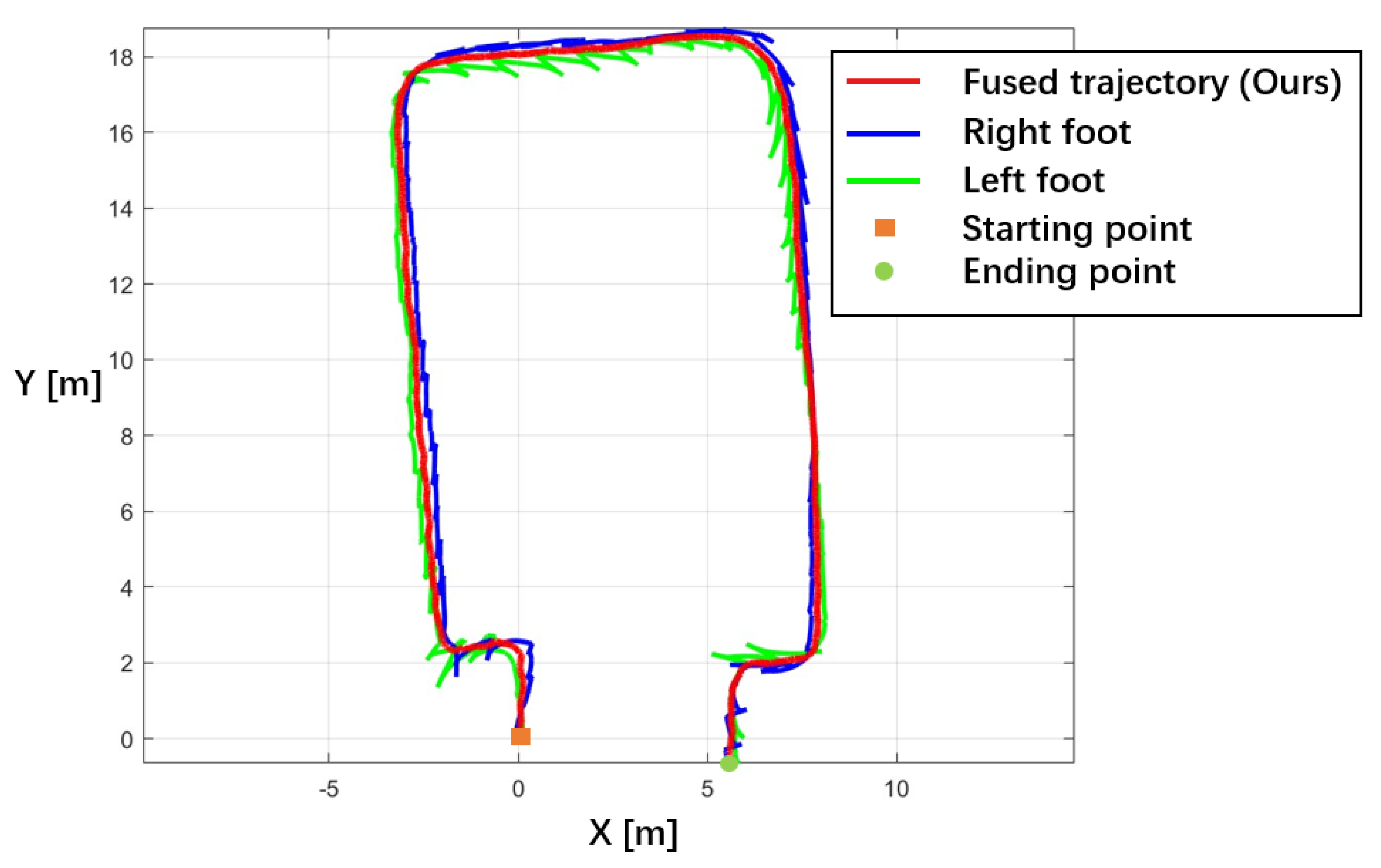
• A novel dual trajectory fusion (DTF) via CBoM projection by replacing the two-foot trajectory with a CBoM-level trajectory using a sine curve weighting method. The fused result demonstrated a stable and smooth trajectory, thereby improving the description of the tracking information.
• An improved dual-foot INS method with minimum centroid distance (MCD) constraining stride length estimation via inner ultrasound ranging and gait analysis. The tracking estimation exhibited a lower RMSE and deviation among all subjects compared with typical approaches.
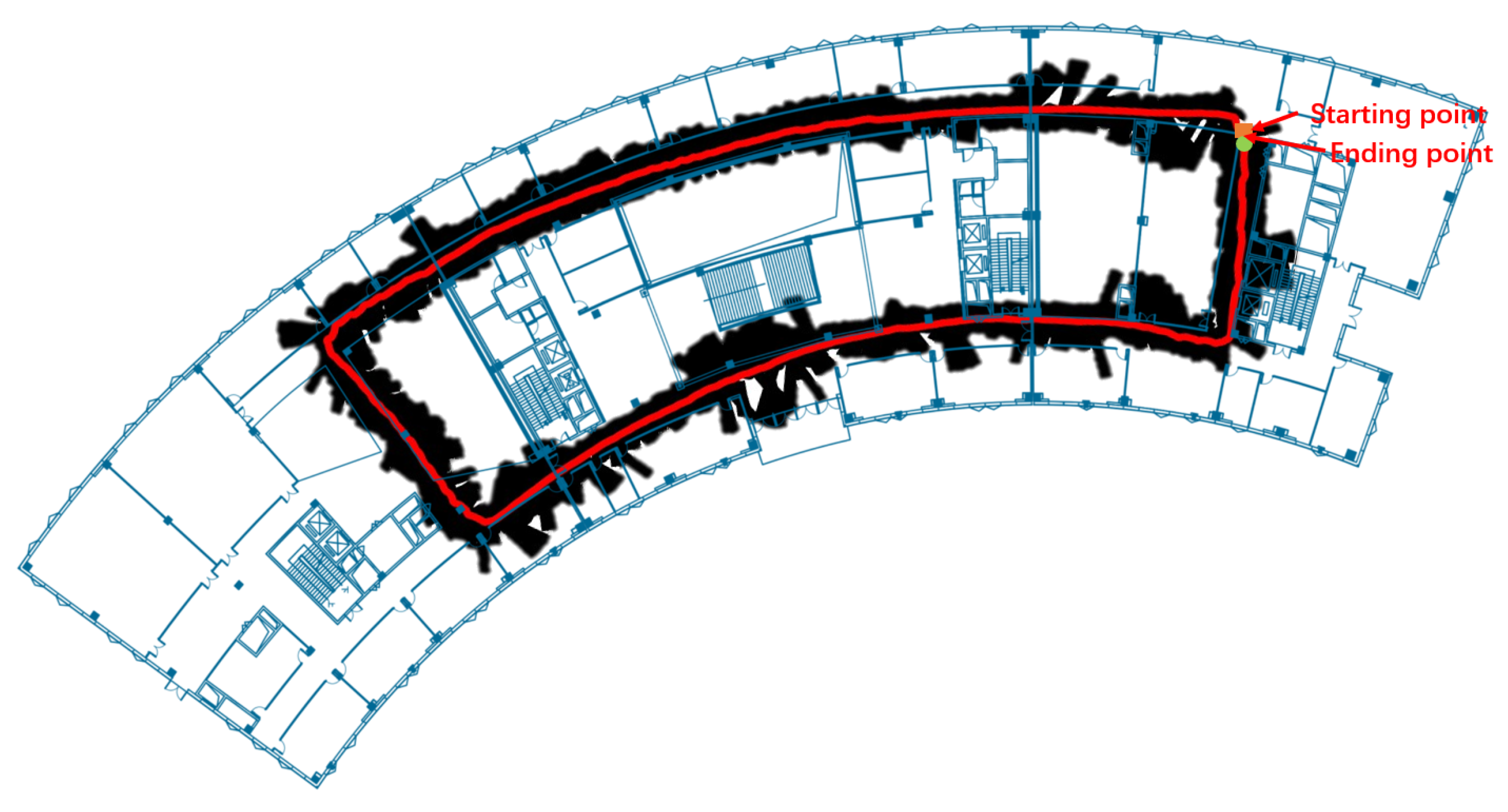
• An ultrasound-ranging-based structure-mapping method that utilizes an occupancy grid map and sphere projection. The mapping results match well with the reference layout, indicating good map reconstruction performance.

The remainder of this study is organized as follows. Section 2 presents an overview of the system, the dual foot-mounted INS algorithm with MCD is presented, the CBoM-based DTF method is described, and the occupancy-grid-map-based ultrasound mapping method is discussed. In Section 3, the proposed methods are analyzed under three different scenarios. In Section 4, the estimation performance is discussed. Finally, Section 5 concludes the study and provides a future research plan.

2. Materials and Methods

In this section, we provide an overview of the IOAM system and introduce the MCD, DTF and S-OGM modules.

2.1. System Overview

This section provides a technical overview (Figure 1) of the proposed IOAM implementation. An IMU and ultrasound sensor were mounted on each shoe. IMU and ultrasound data were obtained from the left and right shoes. In the INS part, IOAM estimates the position of both shoes via kinesiology calculation based on the obtained data [40] and an extended Kalman filter (EKF) is applied for error reduction [21]. The dual-foot position is then filtered under a maximum centroid range constraint via another EKF [41].

The contributions of this study are highlighted in the red boxes in Figure 1, which indicate the novelty of the proposed system. First, IOAM introduces an MCD method that calculates the inner ultrasound-ranging data specifications and determines the dynamic threshold for centroid-method-based dual-foot fusion in INS. In doing so, the dynamic threshold with an accurate stride length constraint improves the tracking estimation performance. Second, this study proposes a DTF method to fuse the two separated trajectories from the two shoes and combine them into one body-level localization information. DTF analyzes the CBoM specifications during movement to determine the weight for left and right trajectory fusion. Finally, a 2D-plane map is projected through outer ultrasound ranging using the sphere projection theory. The map area is obtained via an occupancy grid map (OGM) [42] to calculate the occupancy status of every pixel (clearing/irrelevant). The localization and mapping information is then visualized using a uniform canvas.

2.2. MCD Aided INS for Dual Foot Fusion

2.2.1. EKF Initialization

The state vector ${\widehat{x}}_k^{\left(j\right)}$ of EKF utilized in IOAM is defined as [41]:

$${\widehat{x}}_k^{\left(j\right)}\triangleq {\left[{\widehat{p}}_k^{\left(j\right)}{\widehat{v}}_k^{\left(j\right)}{\widehat{\theta }}_k^{\left(j\right)}\right]}^T$$

(1)

where ${\widehat{p}}_k^{\left(j\right)}\in R^3$, ${\widehat{v}}_k^{\left(j\right)}\in R^3$ and ${\widehat{\theta }}_k^{\left(j\right)}\in R^3$ represent a priori position, velocity, and pose estimation on the three-axis coordinate system [27,28]. There are two EKFs in IOAM for ZUPT and MCD respectively. In this subsection, the determination of ZUPT-EKF and the initialization of MCD-EKF is introduced. The foundamental structure of the EKF is followed with [41] with external definitions for our study (Equations (2)–(5)). Owing to the physical transmission properties of sound and electronic limitations [43], the sampling rate of the ultrasound sensor is lower than that of the IMU. The nearest interpolation method [44] was adopted to align the ultrasound and IMU data, as follows:

$$u^{\left(i\right)\left(j\right)}=\mathrm{interp}\left({\widehat{u}}^{\left(i\right)\left(j\right)},\frac{Ts\left(im{u}^{\left(j\right)}\right)}{Ts\left({\widehat{u}}^{\left(i\right)\left(j\right)}\right)}\right)$$

(2)

where ${\widehat{u}}^{\left(i\right)\left(j\right)}$ and $u^{\left(i\right)\left(j\right)}$ represent the original and interpolated ultrasound range signals, respectively. $i\in \left\{\mathrm{Inner},\mathrm{Outer}\right\}$ represents the placement, that is, the inner and outer sides of the ultrasonic sensors attached to one foot. $j\in \left\{R,L\right\}$ represents sensors mounted on the right or left foot. $Ts$ indicates the sampling rate of the sensor data. Two data sequences from the sensors on each foot were synchronized. The IMU data $D_k^{\left(i\right)}\in R^6$ are defined as:

$$D_k^{\left(j\right)}\triangleq {\left[a_k^{\left(j\right)}{\omega }_k^{\left(j\right)}\right]}^T$$

(3)

where $a_k^{\left(j\right)}\in R^3$ and ${\omega }_k^{\left(j\right)}\in R^3$ represent three-axis acceleration (m/s${}^2$) and angular rate (rad/s${}^2$), respectively. $k\in N^{+}$ indicates the time stamp of the data sequence.

The initial coordinate of the CBoM trajectory from the DTF calculation $p_{COM}$ is defined as:

$$p_{COM}={\left[\begin{array}{ccc}0& 0& 0\end{array}\right]}^T$$

(4)

To separate the dual-foot coordinate calculation, the two feet initial position coordinates $p_1^{\left(j\right)}$ are defined as posteriori by inner ultrasound ranging. The coordinates of $p_1^{\left(L\right)}$ and $p_1^{\left(R\right)}$ are defined as:

$$p_1^{\left(L\right)}={\left[\begin{array}{ccc}-\frac{\mu }{2}& 0& 0\end{array}\right]}^T,p_1^{\left(R\right)}={\left[\begin{array}{ccc}\frac{\mu }{2}& 0& 0\end{array}\right]}^T$$

(5)

where $\mu$ determines the initial x-axis direction stride-length parameter. The dead reckoning process of INS for state transition is defined below:

$${\widehat{x}}_k^{\left(j\right)}=f\left({\widehat{x}}_{k-1}^{\left(j\right)},{\stackrel{\sim }{e}}_{k-1}^{\left(j\right)}\right)$$

(6)

where f denotes the nine-dimensional state transforming function, ${\widehat{x}}_{k-1}^{\left(j\right)}$ denotes the error covariance variable. The state covariance matrix is defined below:

$$P_k^{\left(j\right)}=F_k^{\left(j\right)}{P}_k^{\left(j\right)}{\left(F_k^{\left(j\right)}\right)}^T+G_k^{\left(j\right)}{Q}_k^{\left(j\right)}{\left(G_k^{\left(j\right)}\right)}^T$$

(7)

where $F_k^{\left(j\right)}$ and $G_k^{\left(j\right)}$ denotes the state transition and the noise gain matrix [41]. A step detector [45] classifies each $D_k^{\left(i\right)}$ sample according to its motion state as either moving or stationary. When a stationary phase is detected, the INS sets pseudo-measurements in the EKF to compute the posteriori of the ${\widehat{x}}_k^{\left(j\right)}$ [21,46,47,48].

2.2.2. MCD

The centroid method defines the relative range between the two feet. In a typical dual-foot INS, the distance between two feet has a maximum range constrained by a sphere or ellipsoid model. The distance constraint [41] is described as:

$${∥{\widehat{p}}_k^{\left(R\right)}-{\widehat{p}}_k^{\left(L\right)}∥}_2\le {\gamma }_k,\forall k\in N^{+}$$

(8)

where ${∥∥}_2$ denotes the two-norm calculator, and $\gamma$ is a fixed range threshold. The Lagrange function [49] solution for position pseudo-measurement $p_k^{\left(j\right)}$ under the constrained least squares (CLS) [41,50,51] framework is defined as:

$$\begin{array}{c}\hfill p_k^{\left(R\right)}=\frac{\left({∥{\widehat{p}}_k^{\left(R\right)}-{\widehat{p}}_k^{\left(L\right)}∥}_2+\gamma \right){\widehat{p}}_k^{\left(R\right)}+\left({∥{\widehat{p}}_k^{\left(R\right)}-{\widehat{p}}_k^{\left(L\right)}∥}_2-\gamma \right){\widehat{p}}_k^{\left(L\right)}}{2{∥{\widehat{p}}_k^{\left(R\right)}-{\widehat{p}}_k^{\left(L\right)}∥}_2},\\ \\ \hfill p_k^{\left(L\right)}=\frac{\left({∥{\widehat{p}}_k^{\left(R\right)}-{\widehat{p}}_k^{\left(L\right)}∥}_2+\gamma \right){\widehat{p}}_k^{\left(L\right)}+\left({∥{\widehat{p}}_k^{\left(R\right)}-{\widehat{p}}_k^{\left(L\right)}∥}_2-\gamma \right){\widehat{p}}_k^{\left(R\right)}}{2{∥{\widehat{p}}_k^{\left(R\right)}-{\widehat{p}}_k^{\left(L\right)}∥}_2}\end{array}$$

(9)

Then, the predefined maximum range pseudo-measurement is applied to optimize the foot’s position using the EKF. The maximum range constraint can only address out-of-range drifting problems due to the dynamic stride length during movement and unpredictable gaits from different users. The bias error from position and altitude estimation would also cause trajectory coinciding and crossing problems, reducing the tracking accuracy. A MCD method is proposed to determine the dynamic stride length constraint threshold via inner ultrasound ranging during the mid-swing phase in the gait cycle. The gait cycle during the swing phase of the moving state can be categorized into three continual sub-statuses: initial swing, mid-swing, and terminal swing [52] based on the position of the swinging leg relative to the stationary leg (Figure 2). It is assumed that the normal gait cycle did not involve leg cross-swinging.

In MCD, the mid-swing phase detection can be simply determined as:

$$S_k^{\left(j\right)}=\left\{\begin{array}{c}1,{{\kappa }_{min}<u}_k^{\left(inner\right)\left(j\right)}<{\kappa }_{max}\hfill \\ 0,others\hfill \end{array}\right.$$

(10)

where $\kappa$ is the stride length parameter.To reduce inaccurate measurements during the swinging phase, the inner stride length range is designed to operate in the stance phase of the opposite foot. The DTF algorithm first detects the zero-speed states using the generalized likelihood ratio test (GLRT) [44] which is defined as:

$${ZUPT}_k^{\left(j\right)}=\left\{\begin{array}{c}1,zerospeeddetected\hfill \\ 0,others\hfill \end{array}\right.$$

(11)

Each IMU sample is indicated with either one or zero markers representing the current motion state. The minimum internal sampling strategy (Equation (12)) is utilized in this method to reduce the over-optimization of dual-foot data fusion.

$$t_k-t_{LO}<\sigma$$

(12)

where t is the sample timestamp conversion function, $LO$ represents the last operation of the MCD method, and $\sigma$ is the parameter of the timestamp interval. The flow chart of the proposed MCD method is shown in Figure 3.

In MCD, the x- and y-axis data for pseudo-measurements are utilized in the EKF, whereas the z-axis data (height) are not considered in the ultrasound sensor scanning in the 2D plane, as follows:

$${PM}_k^{\left(j\right)}=\left[\begin{array}{c}{PM}_{k,x}^{\left(j\right)}\\ {PM}_{k,y}^{\left(j\right)}\\ p_{k,z}^{\left(j\right)}\end{array}\right]$$

(13)

where ${PM}_k$ indicates the calculated posteriori centroid distance of the pseudo-measurement in the EKF, and $p_{k,z}^{\left(j\right)}$ represents the original z-axis height information in the INS. Finally, using these pseudo-measurements in the Kalman filter platform, the formulas are described as follows [41]:

$$\begin{array}{c}\hfill K_k^{\left(j\right)}=P_k^{\left(j\right)}{\left(H_p\right)}^T{\left[H_p{P}_k^{\left(j\right)}{\left(H_p\right)}^T+R_p\right]}^{-1}\end{array}$$

(14)

$$\begin{array}{c}\hfill {\widehat{x}}_k^{\left(j\right)}={\widehat{x}}_k^{\left(j\right)}+K_k^{\left(j\right)}\left[p_k^{\left(j\right)}-H_p{\widehat{x}}_k^{\left(j\right)}\right]\end{array}$$

(15)

$$\begin{array}{c}\hfill H_p=\left[I_{3\times 3}{0}_{3\times 3}{0}_{3\times 3}{0}_{3\times 3}{0}_{3\times 3}\right]\end{array}$$

(16)

$$\begin{array}{c}\hfill P_k^{\left(i\right)}=\left[I_{15\times 9}-K_k{H}_p\right]P_k^{\left(j\right)}\end{array}$$

(17)

where $K_k^{\left(j\right)}$ denotes the Kalman gain and $H_p$ the observation transition matrix with pseudo-measurement. $I_{3\times 3}$ denotes the identity matrix and $0_{3\times 3}$ denotes the zero matrix. $R_p$ denotes the noise-covariance matrix of $H_p$.

2.3. Projection of CBoM for DTF

In this study, the dual-foot structure is defined as a rigid body to simplify the tracking visualization and transform the foot path to the user’s trajectory [53,54]. The CBoM is calculated by merging the dual-foot estimated position using the weight fusion [55] method:

$$p_{COM}=g\left[p^{\left(R\right)}{p}^{\left(L\right)}\right]=\alpha p^{\left(R\right)}+\beta p^{\left(L\right)},\alpha +\beta =1$$

(18)

where $p_{COM}\in R^3$ indicates the position of the hypothetical CBoM of the body of the sensor carrier. $\alpha$ and $\beta$ are the weight parameters for the right- and left-foot INS, respectively.

During the swing phase (Figure 2), the heading direction is in the sagittal plane (Figure 4). The CBoM swings at the frontal plane of the body during the alternating movement of the two legs during walking, which can be defined as a pendulum model [56]. The pendulum range can represent the fusion weight, which is defined by a sine function [57,58,59]. The ZUPT clustering method used to calculate the weight is shown in Figure 5.

Where ${ZUPT-j}_m^n$ denotes the ZUPT cluster containing continual zero-speed samples ($ZUPT=1$), m indicates the order number of ZUPT clusters in all input samples, n indicates the order number in a specific ZUPT cluster. Then, the weight of the DTF is defined as:

$$weight=\left\{\begin{array}{cc}0.5+0.25\ast sin\left(\frac{n}{\left.{length\left(ZUPT-L\right.}_m^n\right)}\right)\hfill & ,{ZUPT}^{\left(L\right)}=1\hfill \\ 0.5\hfill & ,{ZUPT}^{\left(L\right)}\oplus {ZUPT}^{\left(R\right)}=1\hfill \\ 0.5+0.25\ast sin\left(\frac{n}{\left.{length\left(ZUPT-R\right.}_m^n\right)}\right)\hfill & ,{ZUPT}^{\left(R\right)}=1\hfill \end{array}\right.$$

(19)

Thus, the $p_{COM}$ calculation according to Equation (18) would be defined as:

$$p_{COM}=weight\ast p^{\left(R\right)}+\left(1-weight\right)p^{\left(L\right)}$$

(20)

The fused trajectory is then filtered through a $\left(1\times \frac{Ts}{2}\right)$ mean filter [61] for small drifting in the motion integral calculation, as follows:

$${\widehat{p}}_{COM,k}=\frac{2\ast \sum p_{COM,k}}{Ts}$$

(21)

2.4. Ultrasound Mapping

2.4.1. Sphere Projection Mechanism

The coordinates of the ultrasound mapping points are calculated based on the step position and the pose estimated by the INS. The range direction of the ultrasound sensor is parallel to the x-axis of the IMU in each foot. To project the 3D scanning onto the 2D XOY coordinate, a polar transform method is described as follows [55,62,63]:

$$M\left(r_k^{\left(i\right)\left(j\right)}\right)=\left[\begin{array}{c}\cos \theta \cos \phi \\ \cos \theta \sin \phi \end{array}\right]$$

(22)

where $\theta$ and $\phi$ denote the pitch and yaw angles in pose estimation, respectively. The coordinates of the ultrasound mapping point $U{p}_k^{\left(i\right)\left(j\right)}$ under the maximum covering principle are calculated as follows:

$$U{p}_k^{\left(i\right)\left(j\right)}={\left[U{x}_k^{\left(i\right)\left(j\right)}U{y}_k^{\left(i\right)\left(j\right)}\right]}^T=\left\{\begin{array}{c}{\left[p_k^{\left(j\right)}+u_k^{\left(i\right)\left(j\right)}diag(1,1)M\left(r_k^{\left(i\right)\left(j\right)}\right)\right]}^T\\ ,i,j=inner,L\left|\right|outer,R\\ {\left[p_k^{\left(j\right)}-u_k^{\left(i\right)\left(j\right)}diag(1,1)M\left(r_k^{\left(i\right)\left(j\right)}\right)\right]}^T\\ ,i,j=inner,R\left|\right|outer,L\end{array}\right.$$

(23)

For the ultrasound ranging, it should satisfy the condition:

$$R_{min}<u_k^{\left(i\right)\left(j\right)}{<R}_{max}$$

(24)

where $R_{min}$ and $R_{max}$ are the ultrasound sensors’ minimum and maximum available measurement ranges (

Table 1. Specifications of MPU9250 IMU.

Operating Voltage	DC 5 V
Accelerometer Scale Range	±16 g
Gyroscope Scale Range	±2000°/s
Communication Interface	I${}^2$C
Sampling Rate	200 Hz

), respectively. The inner ultrasound mapping points should also be calculated at the initial swinging and terminal swinging phrases (Figure 2) and satisfy the $u_k^{\left(inner\right)\left(j\right)}>{\kappa }_{max}$ condition.

2.4.2. S-OGM Calculation

Compared with the laser range finder, the ultrasound sensor has a lower cost and wider detection angle, making it more practical for wearable applications [64]. In addition, ultrasound sensors are stable under smoke- and vapor-filled environments with lower energy consumption among different range measurement methods [43,64]. According to ultrasound specifications, each ranging process is modeled as a rectangular zone (white arrow in Figure 6) in the occupancy grid map (OGM) [42] as follows:

The single grid cells of the map are categorized as empty (black) or irrelevant (gray) areas. The S-OGM algorithm is defined as:

$$B\left(p_k^{\left(j\right)},U{p}_k^{\left(i\right)\left(j\right)}\right)$$

(25)

where $p_k^{\left(j\right)}$ and $U{p}_k^{\left(i\right)\left(j\right)}$ indicate the ultrasound placement position coinciding with the foot position and position of the pixel at the clearing area boundary, respectively.

3. Results

3.1. Experimental Setup

A pair of wearable sensor modules was designed for the data collection. The proposed wearable module is shown in Figure 7a and consists of an MPU9250 IMU (see Table 1), an HC-SR04 ultrasound sensor (see

Table 2. Specifications of HC-SR04 ultrasound sensor.

Operating Voltage	DC 5V
Operating Current	15 mA
Operating Frequency	40 kHz
Range	2 cm–5 m
Ranging Accuracy	3 mm
Measuring Angle	15 degrees
Trigger Input Signal	10 µS TTL Pulse
Sampling rate	15 Hz

), and an ESP32 dual-core microcomputing unit. The module was mounted on the front side of each shoe using a hook and loop tape. The inner ultrasound sensors are staggered and placed separately at the back and front sides of the two shoes to avoid potential ultrasound-emitting interference. A 900 mAh battery with an estimated two-hour power supply was attached to the shoe. Sensor data were transmitted via Wi-Fi to a nearby terminal, as shown in Figure 7b. The data receiver application at the terminal was implemented in MATLAB 2022a using an Intel i7-10510U 1.8 GHz, 16GB RAM laptop.

Eight volunteers were recruited to participate in the experiment, as listed in

Table 3. Height and Weight Information of Volenteers.

Participants Name	Gender	Height (cm)	Weight (kg)
a	male	175	65
b	male	185	85
c	female	163	50
d	female	163	50
e	male	175	70
f	male	172	53
g	male	170	55
h	female	170	47

. Volunteers provided informed consent and the study was approved by the faculty ethics review board. Three scenarios were designed and set up at three different office-like buildings with solid red line reference routes (see Figure 8): a rectangular route (Scenario 1, 161.23 m), a fan-shaped route (Scenario 2, 198.55 m), and a bottle-shaped route (Scenario 3, 53.06 m). Volunteers were requested to wear the designed modules and walk along the pre-arranged route. Start and end points were marked with black sticky tape, placed on the ground. The marker positions were established using a laser range finder and cross-referencing against a computer-aided design (CAD) floor plan. There were no gait or gesture limitations during walking. Each volunteer walked in all three scenarios.

3.2. Trajectory Fusion

The results of DTF are shown in Figure 9. Two single-foot trajectories (blue and green lines) demonstrate serrated lines with estimated stride lengths larger than 1.5 m in the turning phase, showing a significant bias error. In this case, the individual’s position is located at a 1.5-m possibility area, increasing the difficulty of the ILBS visualization. However, the fused trajectory (red line) illustrates one path of the CBoM, which is easy to track and evaluate. Section B’s INS tracking performance evaluation was used to analyze the accuracy of the fused trajectory.

3.3. Tracking Performance

The root-mean-square error (RMSE) [65] was used to evaluate the localization accuracy of the fused trajectory. Scenarios 1 and 2 are closed routes that were used to evaluate the RMSE of the x- and y-axes between the estimated starting and ending points. Scenario 3 contains an open route, which was evaluated by the RMSE of the x-axis (eliminating the ground truth horizontal distance) and the y-axis separately. The bold values indicate results with a relatively lower error. The error rate calculates the ratio of the RMSE error to the route length [66].

3.3.1. Scenario 1

Table 4. Comparison of RMSE [M] of INS Trajectory with and without MCD Constraint for Scenario 1.

	RMSE of INS w/MCD (Ours)	Error Rate (%) w/MCD (Ours)	RMSE of INS w/o MCD	Error Rate (%) w/o MCD
a	0.5379	0.3336	2.1955	1.3617
b	0.3532	0.2191	1.1144	0.6911
c	2.7249	1.6900	6.2353	3.8673
d	0.8919	0.5532	8.4962	5.2696
e	2.7604	1.7121	3.6228	2.2470
f	0.2883	0.1788	1.2563	0.7792
g	0.5602	0.3475	1.0193	0.6322
h	0.3288	0.2039	0.5659	0.3510
Ave./std.	1.06/1.06	0.65/0.67	3.06/2.88	1.90/1.79

illustrates the RMSE and error rate of the Scenario 1 experiment. The proposed method had a lower RMSE (Ave. = 1.06 m) than the method without MCD (Ave. = 3.06 m) for all participants. All participants with MCD had an error rate of less than 2 %, which is acceptable for localization. Participant d (see Figure 10) showed the most significant error rate improvement (0.5532/5.2696). Our trajectory’s starting and ending points coincide more closely than those of the method without MCD. For the result without MCD (blue line), the drifting bias significantly increases from coordinate position (−40,20), which causes a significant bias error at the ending point. The proposed MCD method further constrained the drift of foot position estimation. Thus, the RMSE of the fused trajectory is reduced. The same improvement was also observed in participant a (0.3336/1.3617) and participant c (1.69/3.8673), which proves the versatility of the MCD.

3.3.2. Scenario 2

Scenario 2 comprises two long curved routes, as shown in Figure 8b, which challenges the position estimation of the INS. Our method (shown in

Table 5. Comparison of RMSE [M] of INS Trajectory with and without MCD Constraint for Scenario 2.

	RMSE of INS w/MCD (Ours)	Error Rate (%) w/MCD (Ours)	RMSE of INS w/o MCD	Error Rate (%) w/o MCD
a	6.3940	3.2203	6.8789	3.4646
b	0.3872	0.1950	2.2238	1.1200
c	0.5804	0.2923	1.1148	0.5615
d	1.8863	0.9500	4.9937	2.5151
e	3.9305	1.9796	12.8300	6.4618
f	0.7258	0.3656	4.5777	2.3055
g	1.5246	0.7679	2.6720	1.3458
h	1.2124	0.6106	3.4168	1.7209
Ave./std.	2.08/1.94	1.05/1.04	4.84/3.69	2.44/1.86

) has a lower error rate (Ave. = 1.05 m), and the RMSEs are less than 1 m in participants b, c, and f, indicating that our method significantly outperforms the method without MCD. The standard variance of our method was also less than that of the others, indicating that the MCD method was efficient in reducing the bias error of different participant estimations. The trajectory of participant c (see Figure 11) demonstrates that the proposed MCD method reduces the noise of pose estimation and increases the stability during the curing path walking phase, thereby achieving a lower error rate.

3.3.3. Scenario 3

The separated x-axis and y-axis biases measure the distance between the estimated results and the ground truth. The evaluation of the open path needs to consider the horizontal and vertical bias errors. The results (shown in

Table 6. Comparison of RMSE [M] of INS Trajectory with and without MCD Constraint for Scenario 3.

	RMSE of INS w/MCD x-Axis (Ours)	RMSE of INS w/o MCD x-Axis	RMSE of INS w/MCD (Ours) y-Axis	RMSE of INS w/o MCD y-Axis
a	0.2683	0.9455	0.2487	0.4796
b	0.0555	0.5377	0.5687	0.4673
c	0.1094	0.1302	0.1078	0.1191
d	0.6010	0.6885	0.1635	0.5125
e	0.9144	2.1886	1.1010	0.8462
f	0.8375	1.0648	0.3946	0.2835
g	0.7068	1.1101	0.1102	0.3071
h	0.0859	0.1152	0.5443	1.2367
Ave./std.	0.45/0.36	0.85/0.67	0.40/0.34	0.53/0.36

) indicate that our method outperforms most of the samples, particularly for participants a, g, and h. The average RMSE is less than without MCD both on the x-axis (ours = 0.45, w/o MCD = 0.85) and y-axis (ours = 0.40, w/o MCD = 0.53). For example, the estimated trajectory of participant a (see Figure 12) was closer to the ground truth route. In a few samples, such as participants b and e, the x- or y-axis error was higher than that of the participants without MCD. A possible explanation is the bias caused by the participants’ subjective error between the preset ending (black dot) and the real foot landing place (green dots).

In conclusion, the proposed DTF demonstrated a comprehensive individual trajectory which increases the efficiently of visualization and evaluation. Under this advantage, the proposed method showed improved tracking performance with an error rate of approximately 1% in localization under different types of walking scenarios, and good adaptability with approximately 0.7% standard variance for different participants. The proposed MCD reduces the drifting rate of trajectory estimation and improves the localization accuracy of the INS without the MCD method.

3.4. Mapping Estimation

Two mapping results are presented in this section. Figure 13 shows a mapping for Scenario 1 collected from participant h. Most of the mapping area has good consistency with the ground truth; however, some areas at the corner or empty place show an abrupt cone mapping area because the ultrasound sensors were out of range. The mapping for Scenario 2 (see Figure 14) was collected from participant f, which also showed a closed trajectory with a fully covered corridor area. These results showed clear and recognizable surrounding maps which provide significant references for localization.

3.5. Computation

Table 7. Comparison of mean runtime (ms/frame) of localization and mapping with proposed IOAM with other state-of-the-arts.

Method	Dataset	Localization (ms/f)	Mapping (ms/f)
IOAM	Self-collected dataset	0.26	4.27
Centroid-INS [41]	Self-collected dataset	0.20	-
ORB-SLAM3 [14]	EuRoc	32.45	60.08
SVO [67]	EuRoc	23.4	121.0
PL-SLAM [68]	TUM	51.6	323.85

shows the mean runtime of IOAM’s tracking and mapping in the tested scenarios. The localization computational efficiency of IOAM is comparable to other localization approaches, with a difference of 0.06 ms compared against Centroid-INS. Because fewer data are required for IOAM’s map point calculation, compared to SLAM based approaches, IOAM demonstrates the highest mapping efficiency among the tested methods. The runtime comparison indicates that IOAM is well suited for time critical and embedded device applications.

4. Discussion

This paper introduces a new approach to indoor localization based on an IOAM approach. To our knowledge, this is the first localization and mapping system to implement INS as the odometer, which enables non-vision based localization. The use of inertia and ultrasonic ranging makes the system less affected by unpredictable environmental factors such as weather and motion blur. The combination of INS and S-OGM further broadens the potential application areas for localization under scenarios without prior map information, such as firefighting and elder caring. Additionally, the proposed DTF and MCD contribute valuable dual foot trajectory visualization and error reduction ideas to the research community. Finally, the self-designed wearable costs significantly less than most of the existing approaches, which promotes the development of the corresponding industry.

The results are dependent on a number of factors, which makes it hard to compare them to existing works. Nevertheless, the experimental results are comparable to and in some cases superior to those reported in the literature by some state-of-the-art methods as shown in

Table 8. Position error comparison with state-of-the-art studies.

Ref.	Sensor	Method	Scenario	Performance Metrics
[20]	IMU	INS with closing points and smoothing algorithm; trajectory matching algorithm	1500 m repeated circular path	RMS: 0.5 m
[23]	IMU ADIS16495, cameraDVS128	Dynamic vision assisted zero velocity detector	160 m indoor close-loop route	CEP: 0.9 m
[24]	IMU Memsense Nano	Adaptive stance-phase detection	100 m${}^2$ in a close-loop area	RMSE: 0.85 m
[25]	IMUMIMU22BTP(X), motion capture system	SVM, motion type classifier	1000 m${}^2$ hallway	MEPE: 2.68 m
[26]	IMU InvenSense 20600	DNN-based trajectory reconstruction	Office building on two separate floors (about 1650 and 2475 m${}^2$)	N/A
[27]	IMU MPU9150	Spacial range constraint	indoor building	RMSE > 2 m
[28]	IMU ADIS16448	Multi-sensor fusion for dual-gait analysis	100 m straight route, 345 m rectangle route	RMSE: 2.54 m
[29]	IMUMTi-G710	Adaptive inequality constraints	87.2 m straight route, 120 m L-shaped route	PE: 2.5 m
Ours	IMU MPU9250	MCD	Three different indoor buildings	RMSE: 1.2 m

. The position error is lower in some studies with predefined landmarks [20] or with high quality IMUs [24]. The position error is also lower when external sensor assistance is used [23]. Our method outperforms a study with similar quality IMU [27]. Furthermore, our experiment had the most participants of any other study, which made the human factors, such as subjectivity, less of a factor.

However, limitations in the physical properties of low cost ultrasound sensors often led to inaccurate stride length measurements, which in turn affected the tracking performance. Several mappings were impacted due to noise in the data when the measurement was out of range, leading to incorrect boundary predictions. Furthermore, the accuracy of range measurements can also be affected by uneven ultrasonic reflective planes, which can affect mapping performance at the corners and empty areas. To overcome this limitation, the combination of ranging methods will be adopted in the future study.

5. Conclusions

This study proposes IOAM, a novel localization and mapping approach that integrates DF-INS and ultrasound sensors. The primary contributions of this work include the proposal of a MCD in the EKF to reduce the fusion bias error, a DTF method to fuse two-foot trajectories to the CBoM trajectory, and an ultrasound mapping method to reconstruct the S-OGM simultaneously. The estimated results indicate a lower RMSE and error rate than the traditional method, and the mapping area primarily covers the reference layout, demonstrating good map reconstruction performance. Future work will explore the application of hybrid ranging sensors for longer-range measurements and the IOAM combination of multiple users for a broad application potential.

References

1. Basiri, A.; Lohan, E.S.; Moore, T.; Winstanley, A.; Peltola, P.; Hill, C.; Amirian, P.; e Silva, P.F. Indoor location based services challenges, requirements and usability of current solutions. Comput. Sci. Rev. 2017, 24, 1–12. [Google Scholar] [CrossRef] [Green Version]
2. Pirzada, N.; Nayan, M.Y.; Subhan, F.; Hassan, M.F.; Khan, M.A. Comparative analysis of active and passive indoor localization systems. Aasri Procedia 2013, 5, 92–97. [Google Scholar] [CrossRef]
3. Zhu, N.; Marais, J.; Bétaille, D.; Berbineau, M. GNSS position integrity in urban environments: A review of literature. IEEE Trans. Intell. Transp. Syst. 2018, 19, 2762–2778. [Google Scholar] [CrossRef] [Green Version]
4. Zwirello, L.; Schipper, T.; Harter, M.; Zwick, T. UWB localization system for indoor applications: Concept, realization and analysis. J. Electr. Comput. Eng. 2012, 2012, 849638. [Google Scholar] [CrossRef] [Green Version]
5. Kotaru, M.; Joshi, K.; Bharadia, D.; Katti, S. Spotfi: Decimeter level localization using wifi. In Proceedings of the 2015 ACM Conference on Special Interest Group on Data Communication, London, UK, 17–21 August 2015; pp. 269–282. [Google Scholar]
6. Ssekidde, P.; Steven Eyobu, O.; Han, D.S.; Oyana, T.J. Augmented CWT features for deep learning-based indoor localization using WiFi RSSI data. Appl. Sci. 2021, 11, 1806. [Google Scholar] [CrossRef]
7. Thaljaoui, A.; Val, T.; Nasri, N.; Brulin, D. BLE localization using RSSI measurements and iRingLA. In Proceedings of the 2015 IEEE International Conference on Industrial Technology (ICIT), Seville, Spain, 17–19 March 2015; pp. 2178–2183. [Google Scholar]
8. Zhou, J.; Shi, J. RFID localization algorithms and applications—A review. J. Intell. Manuf. 2009, 20, 695–707. [Google Scholar] [CrossRef]
9. Monica, S.; Ferrari, G. UWB-based localization in large indoor scenarios: Optimized placement of anchor nodes. IEEE Trans. Aerosp. Electron. Syst. 2015, 51, 987–999. [Google Scholar] [CrossRef] [Green Version]
10. Castle, R.O.; Gawley, D.J.; Klein, G.; Murray, D.W. Towards simultaneous recognition, localization and mapping for hand-held and wearable cameras. In Proceedings of the 2007 IEEE International Conference on Robotics and Automation, Roma, Italy, 10–14 April 2007; pp. 4102–4107. [Google Scholar]
11. Taketomi, T.; Uchiyama, H.; Ikeda, S. Visual SLAM algorithms: A survey from 2010 to 2016. IPSJ Trans. Comput. Vis. Appl. 2017, 9, 16. [Google Scholar] [CrossRef] [Green Version]
12. Wu, R.; Pike, M.; Lee, B.G. DT-SLAM: Dynamic Thresholding Based Corner Point Extraction in SLAM System. IEEE Access 2021, 9, 91723–91729. [Google Scholar] [CrossRef]
13. Poulose, A.; Han, D.S. Hybrid indoor localization using IMU sensors and smartphone camera. Sensors 2019, 19, 5084. [Google Scholar] [CrossRef]
14. Campos, C.; Elvira, R.; Rodríguez, J.J.G.; Montiel, J.M.; Tardós, J.D. Orb-slam3: An accurate open-source library for visual, visual–inertial, and multimap slam. IEEE Trans. Robot. 2021, 37, 1874–1890. [Google Scholar] [CrossRef]
15. Shin, Y.S.; Kim, A. Sparse depth enhanced direct thermal-infrared SLAM beyond the visible spectrum. IEEE Robot. Autom. Lett. 2019, 4, 2918–2925. [Google Scholar] [CrossRef] [Green Version]
16. Khan, M.U.; Zaidi, S.A.A.; Ishtiaq, A.; Bukhari, S.U.R.; Samer, S.; Farman, A. A comparative survey of lidar-slam and lidar based sensor technologies. In Proceedings of the 2021 Mohammad Ali Jinnah University International Conference on Computing (MAJICC), Karachi, Pakistan, 15–17 July 2021; pp. 1–8. [Google Scholar]
17. Mandischer, N.; Eddine, S.C.; Huesing, M.; Corves, B. Radar slam for autonomous indoor grinding. In Proceedings of the 2020 IEEE Radar Conference (RadarConf20), Florence, Italy, 21–25 September 2020; pp. 1–6. [Google Scholar]
18. Bailey, T.; Durrant-Whyte, H. Simultaneous localization and mapping (SLAM): Part II. IEEE Robot. Autom. Mag. 2006, 13, 108–117. [Google Scholar] [CrossRef] [Green Version]
19. Chang, L.; Qin, F.; Jiang, S. Strapdown inertial navigation system initial alignment based on modified process model. IEEE Sens. J. 2019, 19, 6381–6391. [Google Scholar] [CrossRef]
20. Niu, X.; Liu, T.; Kuang, J.; Zhang, Q.; Guo, C. Pedestrian Trajectory Estimation Based on Foot-Mounted Inertial Navigation System for Multistory Buildings in Postprocessing Mode. IEEE Internet Things J. 2021, 9, 6879–6892. [Google Scholar] [CrossRef]
21. Nilsson, J.O.; Skog, I.; Händel, P.; Hari, K. Foot-mounted INS for everybody-an open-source embedded implementation. In Proceedings of the 2012 IEEE/ION Position, Location and Navigation Symposium, Savannah, GA, USA, 11–14 April 2016; pp. 140–145. [Google Scholar]
22. Nilsson, J.O.; Gupta, A.K.; Händel, P. Foot-mounted inertial navigation made easy. In Proceedings of the 2014 International Conference on Indoor Positioning and Indoor Navigation (IPIN), Beijing, China, 27–30 October 2014; pp. 24–29. [Google Scholar]
23. Jao, C.S.; Stewart, K.; Conradt, J.; Neftci, E.; Shkel, A. Zero velocity detector for foot-mounted inertial navigation system assisted by a dynamic vision sensor. In Proceedings of the 2020 DGON Inertial Sensors and Systems (ISS), Braunschweig, Germany, 15–16 September 2020; pp. 1–18. [Google Scholar]
24. Wang, Z.; Zhao, H.; Qiu, S.; Gao, Q. Stance-phase detection for ZUPT-aided foot-mounted pedestrian navigation system. IEEE/ASME Trans. Mechatronics 2015, 20, 3170–3181. [Google Scholar] [CrossRef]
25. Wagstaff, B.; Peretroukhin, V.; Kelly, J. Improving foot-mounted inertial navigation through real-time motion classification. In Proceedings of the 2017 International Conference on Indoor Positioning and Indoor Navigation (IPIN), Sapporo, Japan, 18–21 September 2017; pp. 1–8. [Google Scholar]
26. Chen, C.; Zhao, P.; Lu, C.X.; Wang, W.; Markham, A.; Trigoni, N. Deep-learning-based pedestrian inertial navigation: Methods, data set, and on-device inference. IEEE Internet Things J. 2020, 7, 4431–4441. [Google Scholar] [CrossRef] [Green Version]
27. Prateek, G.; Girisha, R.; Hari, K.; Händel, P. Data fusion of dual foot-mounted INS to reduce the systematic heading drift. In Proceedings of the 2013 4th International Conference on Intelligent Systems, Modelling and Simulation, Washington, DC, USA, 29–31 January 2013; pp. 208–213. [Google Scholar]
28. Zhao, H.; Wang, Z.; Qiu, S.; Shen, Y.; Zhang, L.; Tang, K.; Fortino, G. Heading drift reduction for foot-mounted inertial navigation system via multi-sensor fusion and dual-gait analysis. IEEE Sens. J. 2018, 19, 8514–8521. [Google Scholar] [CrossRef]
29. Wang, Q.; Cheng, M.; Noureldin, A.; Guo, Z. Research on the improved method for dual foot-mounted Inertial/Magnetometer pedestrian positioning based on adaptive inequality constraints Kalman Filter algorithm. Measurement 2019, 135, 189–198. [Google Scholar] [CrossRef]
30. Ye, L.; Yang, Y.; Jing, X.; Li, H.; Yang, H.; Xia, Y. Altimeter+ INS/giant LEO constellation dual-satellite integrated navigation and positioning algorithm based on similar ellipsoid model and UKF. Remote. Sens. 2021, 13, 4099. [Google Scholar] [CrossRef]
31. Niu, X.; Li, Y.; Kuang, J.; Zhang, P. Data fusion of dual foot-mounted IMU for pedestrian navigation. IEEE Sens. J. 2019, 19, 4577–4584. [Google Scholar] [CrossRef]
32. Chen, C.; Jao, C.S.; Shkel, A.M.; Kia, S.S. UWB Sensor Placement for Foot-to-Foot Ranging in Dual-Foot-Mounted ZUPT-Aided INS. IEEE Sens. Lett. 2022, 6, 5500104. [Google Scholar] [CrossRef]
33. Kingma, I.; Toussaint, H.M.; Commissaris, D.A.; Hoozemans, M.J.; Ober, M.J. Optimizing the determination of the body center of mass. J. Biomech. 1995, 28, 1137–1142. [Google Scholar] [CrossRef] [PubMed]
34. Pai, Y.C.; Patton, J. Center of mass velocity-position predictions for balance control. J. Biomech. 1997, 30, 347–354. [Google Scholar] [CrossRef] [PubMed]
35. Pavei, G.; Seminati, E.; Cazzola, D.; Minetti, A.E. On the estimation accuracy of the 3D body center of mass trajectory during human locomotion: Inverse vs. forward dynamics. Front. Physiol. 2017, 8, 129. [Google Scholar] [CrossRef] [Green Version]
36. Yang, C.X. Low-cost experimental system for center of mass and center of pressure measurement (June 2018). IEEE Access 2018, 6, 45021–45033. [Google Scholar] [CrossRef]
37. Pavei, G.; Salis, F.; Cereatti, A.; Bergamini, E. Body center of mass trajectory and mechanical energy using inertial sensors: A feasible stride? Gait Posture 2020, 80, 199–205. [Google Scholar] [CrossRef]
38. Zhou, B.; Ma, W.; Li, Q.; El-Sheimy, N.; Mao, Q.; Li, Y.; Gu, F.; Huang, L.; Zhu, J. Crowdsourcing-based indoor mapping using smartphones: A survey. Isprs J. Photogramm. Remote. Sens. 2021, 177, 131–146. [Google Scholar] [CrossRef]
39. Matsuki, H.; Scona, R.; Czarnowski, J.; Davison, A.J. Codemapping: Real-time dense mapping for sparse slam using compact scene representations. IEEE Robot. Autom. Lett. 2021, 6, 7105–7112. [Google Scholar] [CrossRef]
40. Woodman, O.J. An Introduction to Inertial Navigation; Report; University of Cambridge, Computer Laboratory: Cambridge, UK, 2007. [Google Scholar]
41. Girisha, R.; Prateek, G.; Hari, K.; Händel, P. Fusing the navigation information of dual foot-mounted zero-velocity-update-aided inertial navigation systems. In Proceedings of the 2014 International Conference on Signal Processing and Communications (SPCOM), Bangalore, India, 22–25 July 2014; pp. 1–6. [Google Scholar]
42. Thrun, S. Learning occupancy grid maps with forward sensor models. Auton. Robot. 2003, 15, 111–127. [Google Scholar] [CrossRef]
43. Chu, B. Position compensation algorithm for omnidirectional mobile robots and its experimental evaluation. Int. J. Precis. Eng. Manuf. 2017, 18, 1755–1762. [Google Scholar] [CrossRef]
44. Rukundo, O.; Cao, H. Nearest neighbor value interpolation. arXiv 2012, arXiv:1211.1768. [Google Scholar]
45. Skog, I.; Handel, P.; Nilsson, J.O.; Rantakokko, J. Zero-velocity detection—An algorithm evaluation. IEEE Trans. Biomed. Eng. 2010, 57, 2657–2666. [Google Scholar] [CrossRef] [PubMed]
46. Fischer, C.; Sukumar, P.T.; Hazas, M. Tutorial: Implementing a pedestrian tracker using inertial sensors. IEEE Pervasive Comput. 2012, 12, 17–27. [Google Scholar] [CrossRef]
47. Rajagopal, S. Personal Dead Reckoning System with Shoe Mounted Inertial Sensors. Master’s Thesis, KTH Electrical Engineering, Stockholm, Sweden, 2008. [Google Scholar]
48. Foxlin, E. Pedestrian tracking with shoe-mounted inertial sensors. IEEE Comput. Graph. Appl. 2005, 25, 38–46. [Google Scholar] [CrossRef]
49. Bector, C.; Chandra, S. On incomplete Lagrange function and saddle point optimality criteria in mathematical programming. J. Math. Anal. Appl. 2000, 251, 2–12. [Google Scholar] [CrossRef] [Green Version]
50. Gander, W. Least squares with a quadratic constraint. Numer. Math. 1980, 36, 291–307. [Google Scholar] [CrossRef]
51. Liew, C.K. Inequality constrained least-squares estimation. J. Am. Stat. Assoc. 1976, 71, 746–751. [Google Scholar] [CrossRef]
52. Jacquelin Perry, M. Gait Analysis: Normal and Pathological Function; SLACK: Thorofare, NJ, USA, 2010. [Google Scholar]
53. Aggarwal, J.K.; Cai, Q. Human motion analysis: A review. Comput. Vis. Image Underst. 1999, 73, 428–440. [Google Scholar] [CrossRef]
54. Posa, M.; Cantu, C.; Tedrake, R. A direct method for trajectory optimization of rigid bodies through contact. Int. J. Robot. Res. 2014, 33, 69–81. [Google Scholar] [CrossRef] [Green Version]
55. Wu, R.; Pike, M.; Chai, X.; Lee, B.G.; Wu, X. SLAM-ING: A Wearable SLAM Inertial NaviGation System. In Proceedings of the 2022 IEEE SENSORS Conference, Dallas, TX, USA, 30 October–2 November 2022. [Google Scholar]
56. Komura, T.; Nagano, A.; Leung, H.; Shinagawa, Y. Simulating pathological gait using the enhanced linear inverted pendulum model. IEEE Trans. Biomed. Eng. 2005, 52, 1502–1513. [Google Scholar] [CrossRef] [PubMed]
57. Buczek, F.L.; Cooney, K.M.; Walker, M.R.; Rainbow, M.J.; Concha, M.C.; Sanders, J.O. Performance of an inverted pendulum model directly applied to normal human gait. Clin. Biomech. 2006, 21, 288–296. [Google Scholar] [CrossRef] [PubMed]
58. Zhou, L.; Liu, J. A method of the body of mass trajectory for human gait analysis. Inf. Technol. 2016, 40, 147–150. [Google Scholar]
59. Shi, Y.; Meng, L.; Chen, D. Human standing-up trajectory model and experimental study on center-of-mass velocity. Proc. IOP Conf. Ser. Mater. Sci. Eng. 2019, 612, 022088. [Google Scholar] [CrossRef]
60. Whittle, M.W. Three-dimensional motion of the center of gravity of the body during walking. Hum. Mov. Sci. 1997, 16, 347–355. [Google Scholar] [CrossRef]
61. Tsai, F.; Philpot, W. Derivative analysis of hyperspectral data. Remote. Sens. Environ. 1998, 66, 41–51. [Google Scholar] [CrossRef]
62. Burger, H.A. Use of Euler-rotation angles for generating antenna patterns. IEEE Antennas Propag. Mag. 1995, 37, 56–63. [Google Scholar] [CrossRef]
63. Weisstein, E.W. Euler Angles. 2009. Available online: https://mathworld.wolfram.com/ (accessed on 20 June 2022).
64. Qiu, Z.; Lu, Y.; Qiu, Z. Review of Ultrasonic Ranging Methods and Their Current Challenges. Micromachines 2022, 13, 520. [Google Scholar] [CrossRef]
65. Chai, T.; Draxler, R.R. Root mean square error (RMSE) or mean absolute error (MAE). Geosci. Model Dev. Discuss. 2014, 7, 1525–1534. [Google Scholar]
66. Shi, W.; Wang, Y.; Wu, Y. Dual MIMU pedestrian navigation by inequality constraint Kalman filtering. Sensors 2017, 17, 427. [Google Scholar] [CrossRef]
67. Forster, C.; Zhang, Z.; Gassner, M.; Werlberger, M.; Scaramuzza, D. SVO: Semidirect visual odometry for monocular and multicamera systems. IEEE Trans. Robot. 2016, 33, 249–265. [Google Scholar] [CrossRef]
68. Pumarola, A.; Vakhitov, A.; Agudo, A.; Sanfeliu, A.; Moreno-Noguer, F. PL-SLAM: Real-time monocular visual SLAM with points and lines. In Proceedings of the 2017 IEEE International Conference on Robotics and Automation (ICRA), Singapore, 29 May–3 June 2017; pp. 4503–4508. [Google Scholar]
Figure 1. System overveiw of IOAM.
Remotesensing 14 06081 g001
Figure 2. Schematic of right foot swing and inner ultrasound sensor scanning process.
Remotesensing 14 06081 g002
Figure 3. Process of MCD algorithm.
Remotesensing 14 06081 g003
Figure 4. Determination of the CBoM [60].
Remotesensing 14 06081 g004
Figure 5. Calculation of ZUPT clustering.
Remotesensing 14 06081 g005
Figure 6. Schematic of ultrasound S-OGM process with five footsteps.
Remotesensing 14 06081 g006
Figure 7. Component layout of IOAM wearable devices (a) and data transmission schematic during the experiment (b).
Remotesensing 14 06081 g007
Figure 8. Layout of data collection locations for scenarios 1 (a), 2 (b), and 3 (c).
Remotesensing 14 06081 g008
Figure 9. 2D plotting of the single foot and dual fused trajectory of Scenario 3 participant b.
Remotesensing 14 06081 g009
Figure 10. 2D plotting of the fused trajectory with MCD (red line) and without MCD (blue line) of Scenario 1 participant d.
Remotesensing 14 06081 g010
Figure 11. 2D plotting of the fused trajectory with MCD (red line) and without MCD (blue line) of Scenario2 participant c.
Remotesensing 14 06081 g011
Figure 12. 2D plotting of the fused trajectory with MCD (red line) and without MCD (blue line) of Scenario 3 participant a.
Remotesensing 14 06081 g012
Figure 13. Plotting the 2D mapping result of Scenario 1; the red line represents the individual’s position, and the black area represents the mapping results.
Remotesensing 14 06081 g013
Figure 14. Plotting of 2D mapping result of Scenario 2.
Remotesensing 14 06081 g014