A Morphing-Based Method for Paleotopographic Reconstruction of the Transverse Canyon


Abstract
:1. Introduction
2. Analysis of the Transverse Canyon
2.1. Characteristics of the Transverse Canyon
- Even without a level floor, the canyon slope is steep, and the canyon bottom is narrow. Due to intense erosion, the majority of transverse canyons are V-shaped, but a handful are U-shaped.
- The mountains spanned by transverse canyons are mostly long or spindle-shaped, and they are the consequence of tectonic uplifts, such as anticline mountains or fault-block mountains with distinct mountain ranges.
- The extension directions of transverse canyons are orthogonal to the mountain strike, or nearly orthogonal.
- Transverse canyons are generated primarily by river capture and headward erosion.
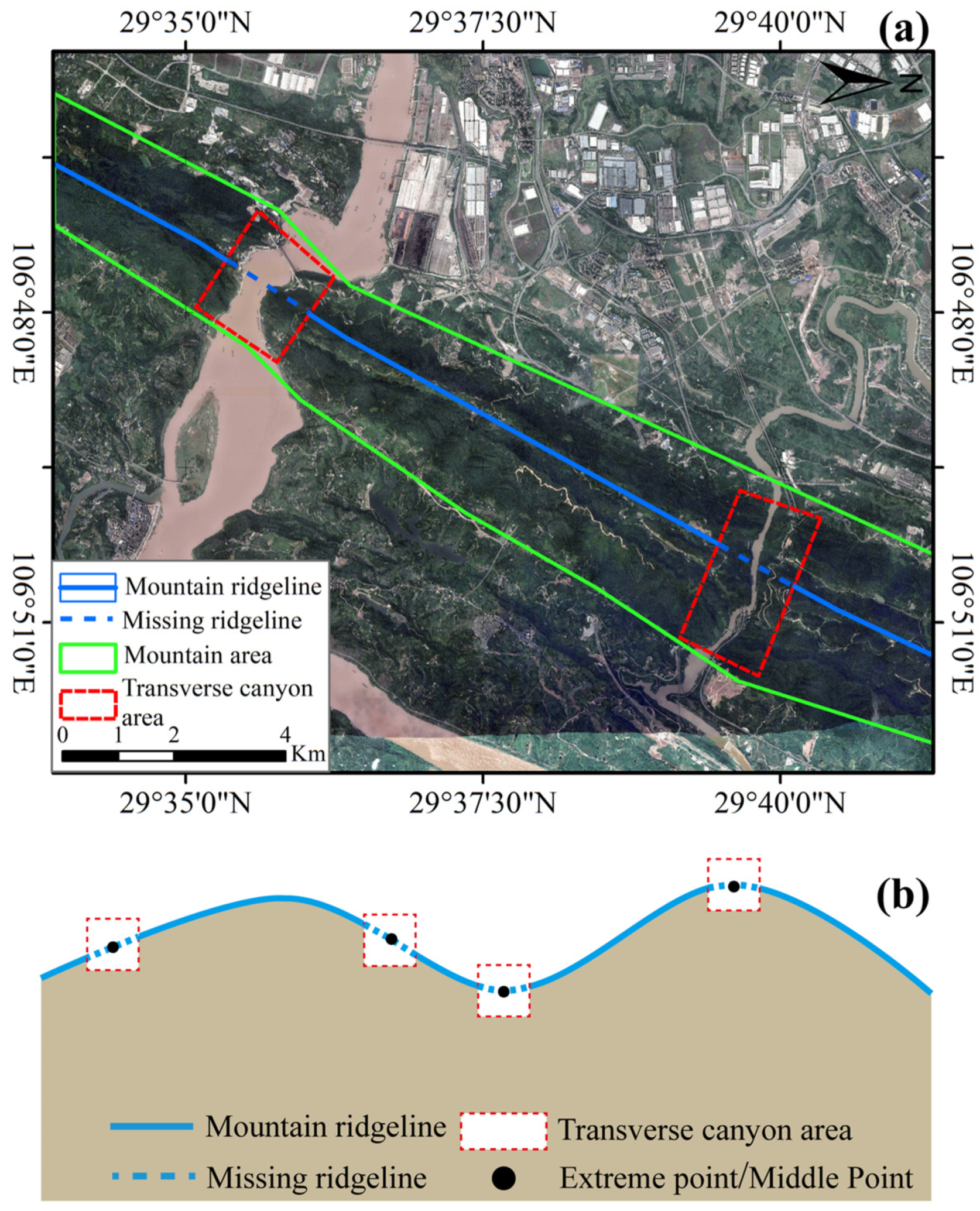
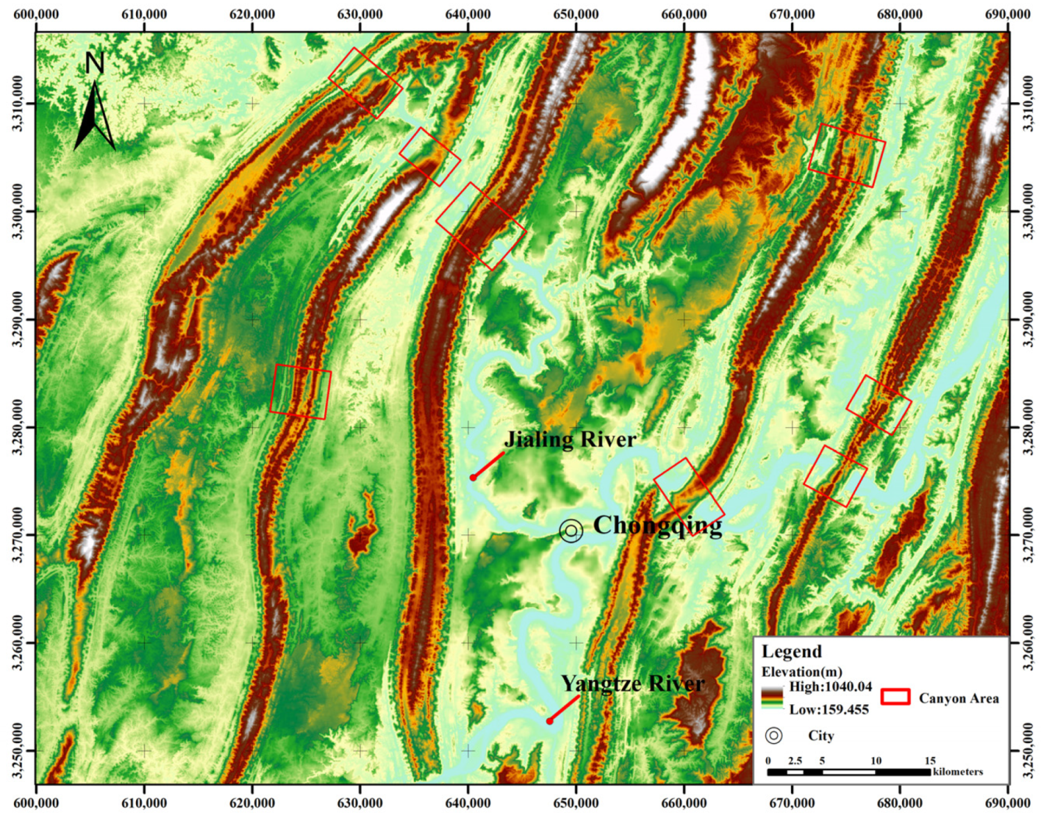
2.2. Locations of the Transverse Canyon
3. Study Region and Input Data
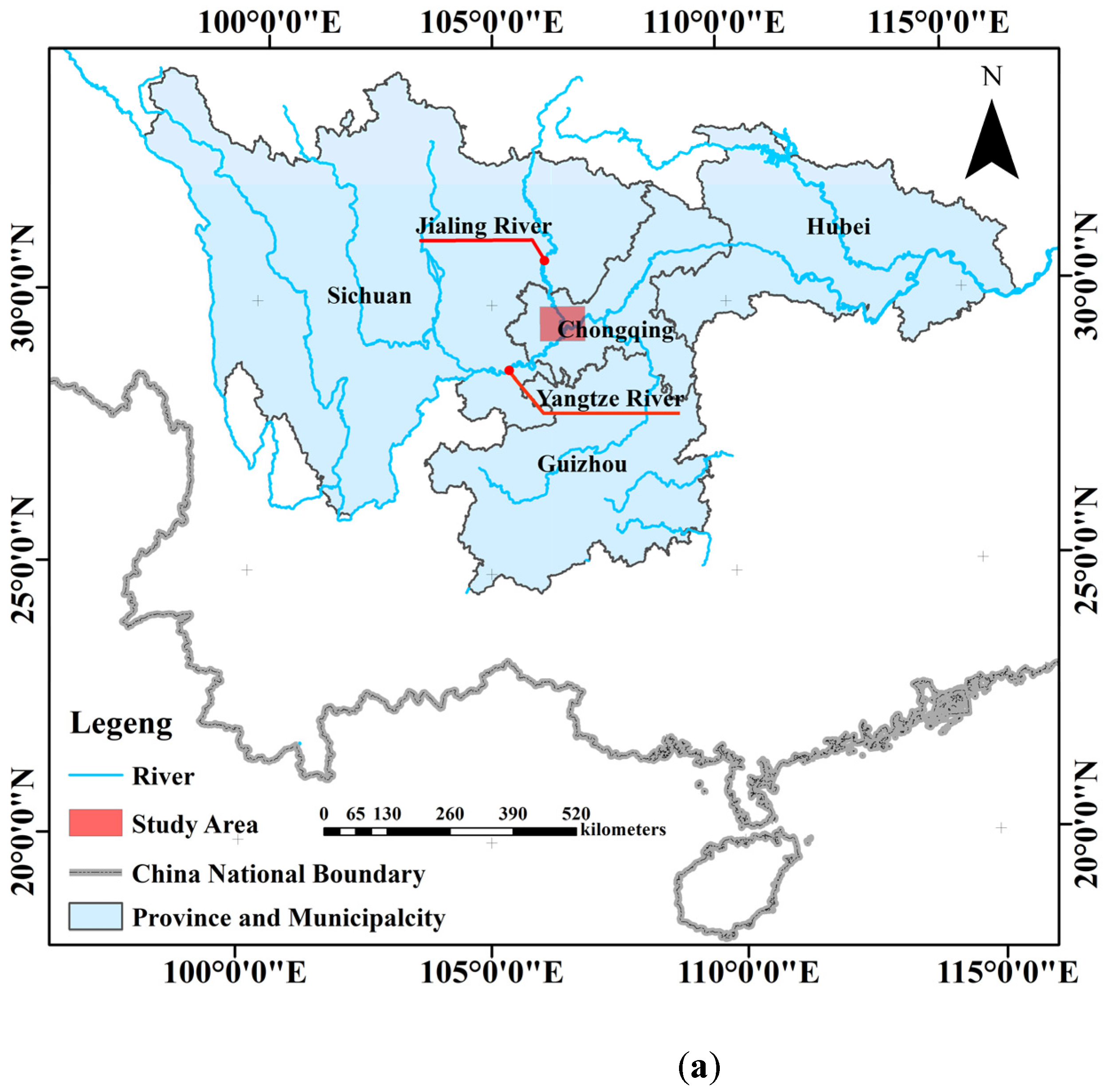
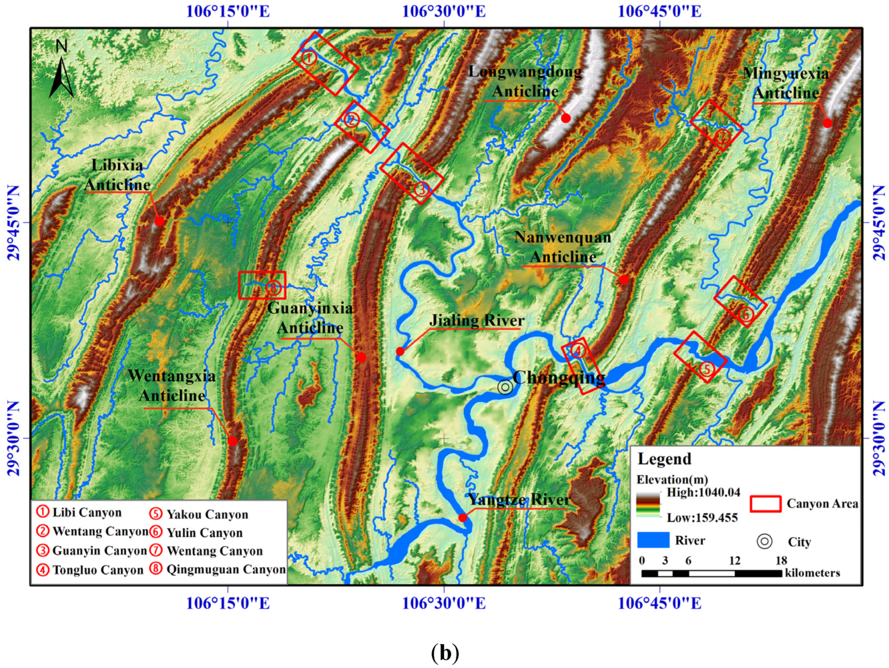
3.1. Study Region
3.2. Input Data
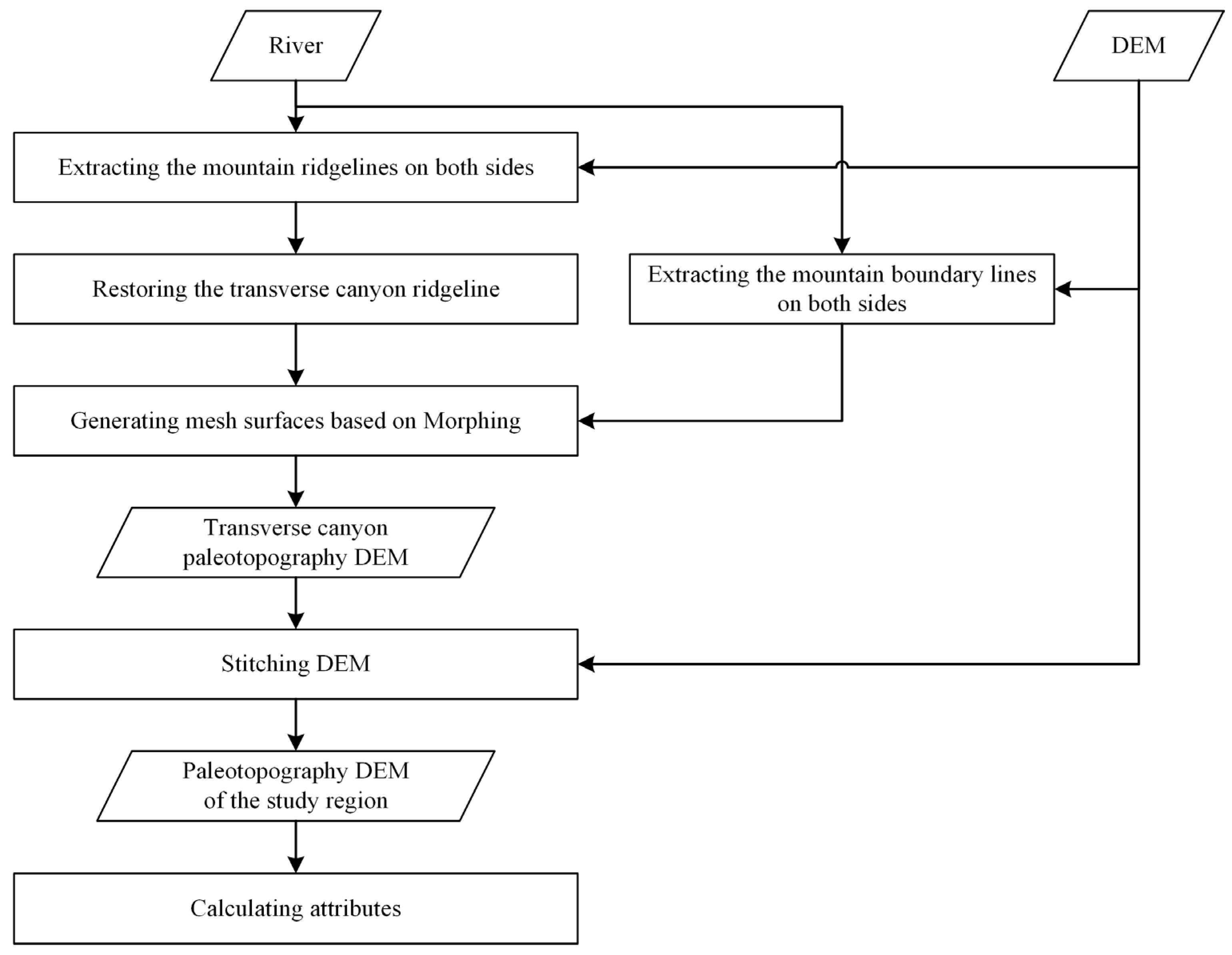
4. Methodology
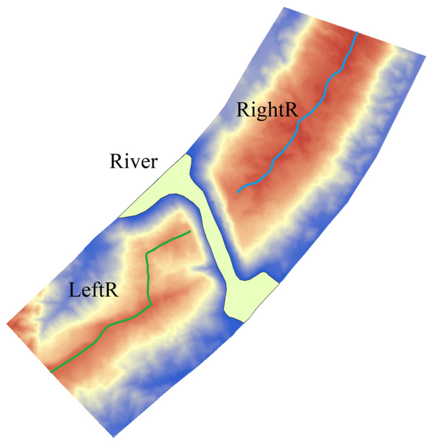
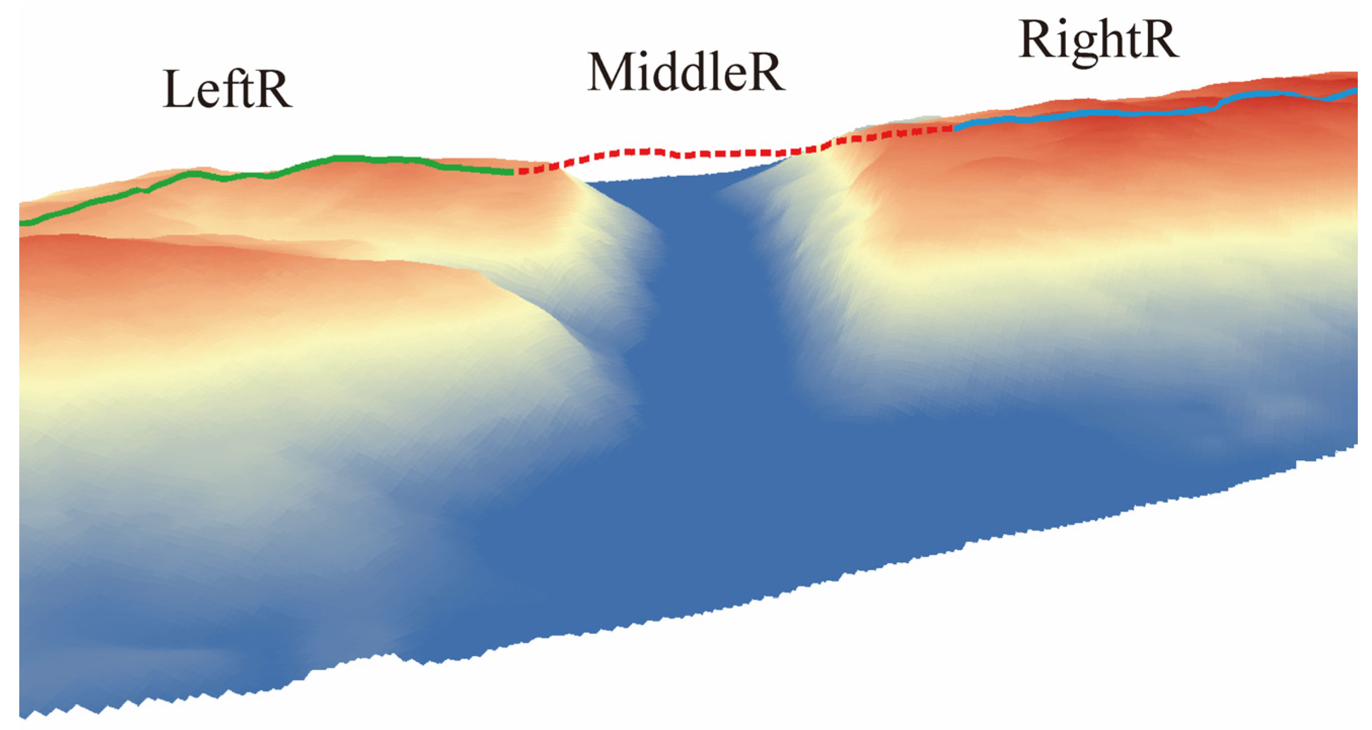
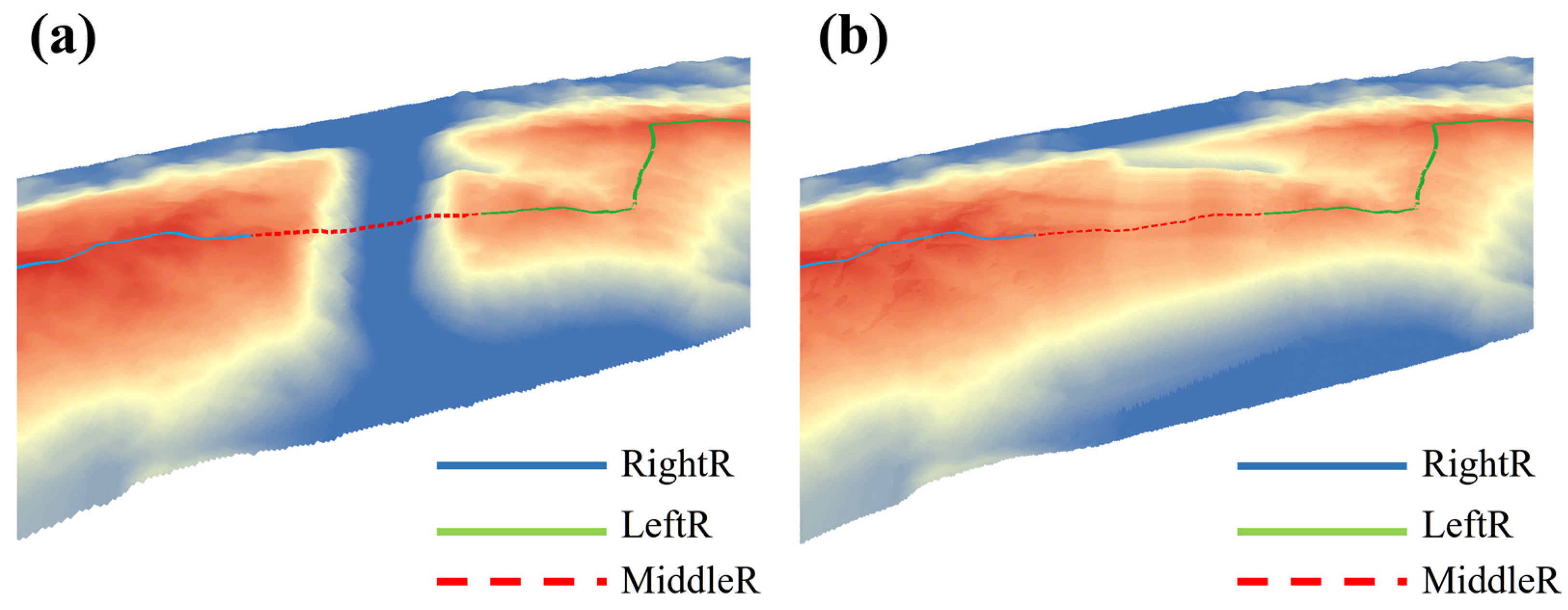
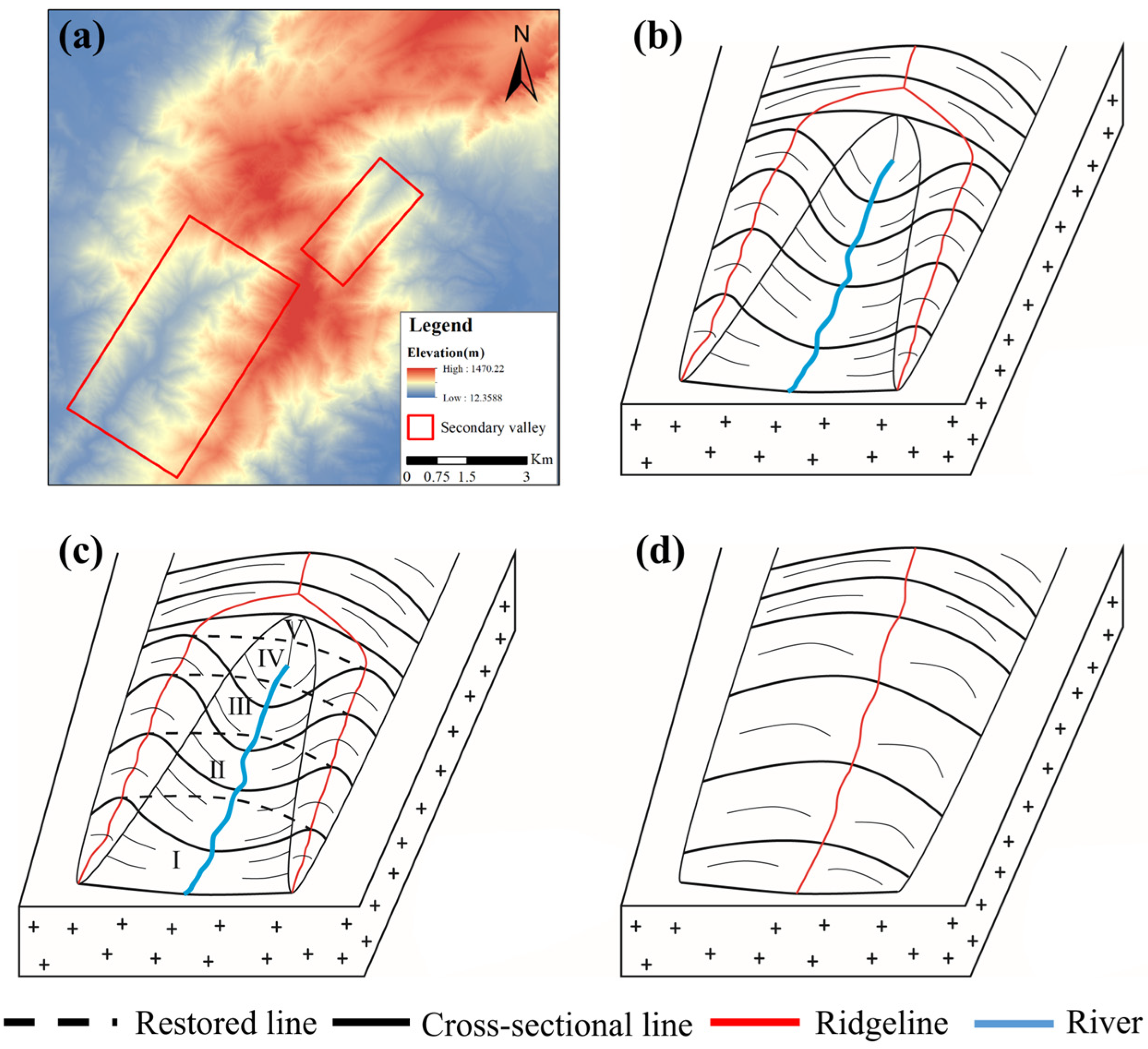
4.1. Restoring the Ridgeline above the Transverse Canyon
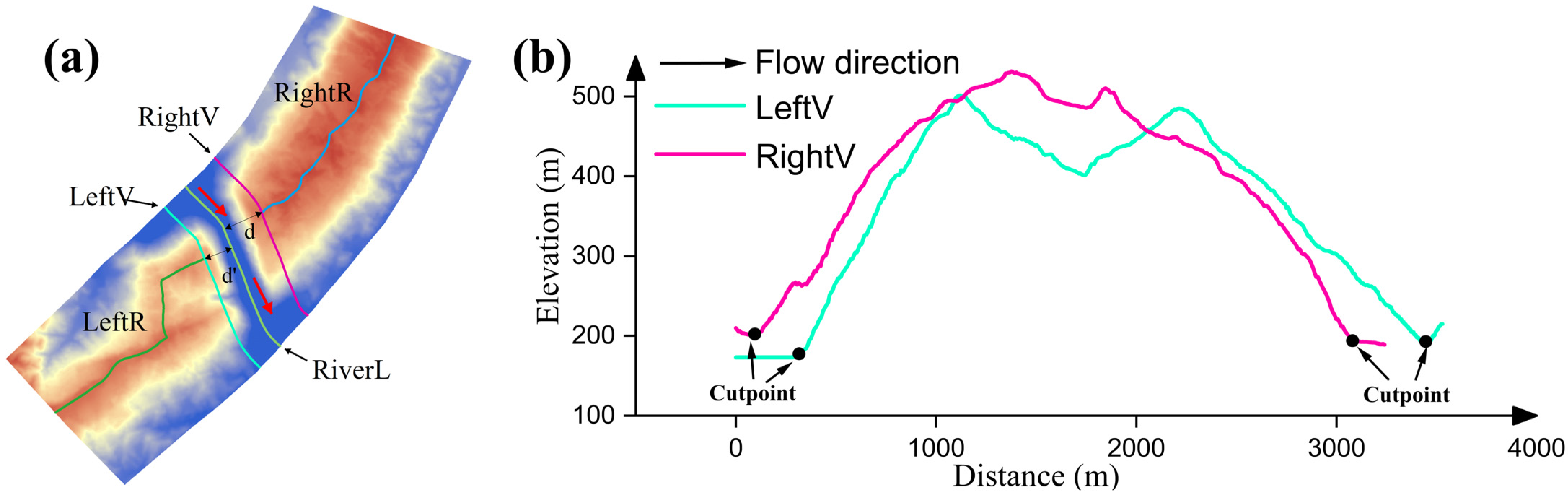
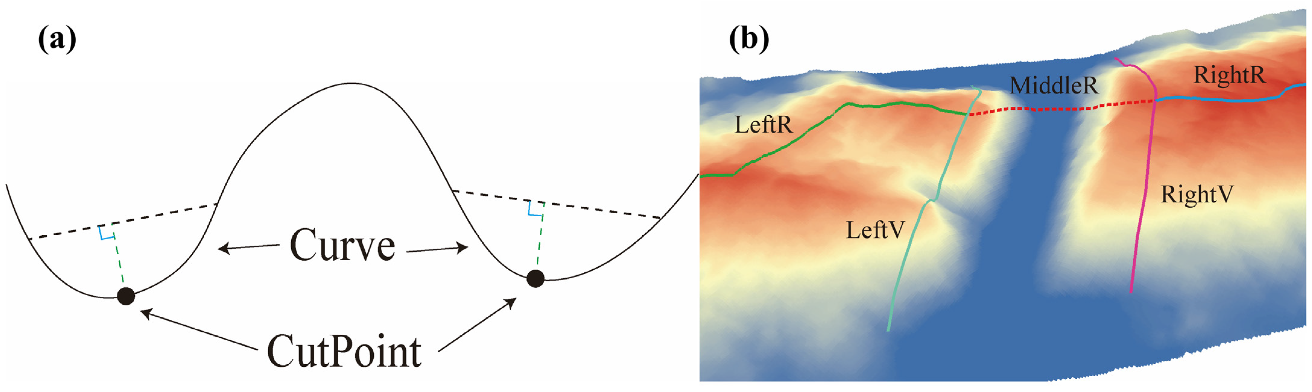
4.2. Generating the Boundary Lines on Both Sides of the Transverse Canyon
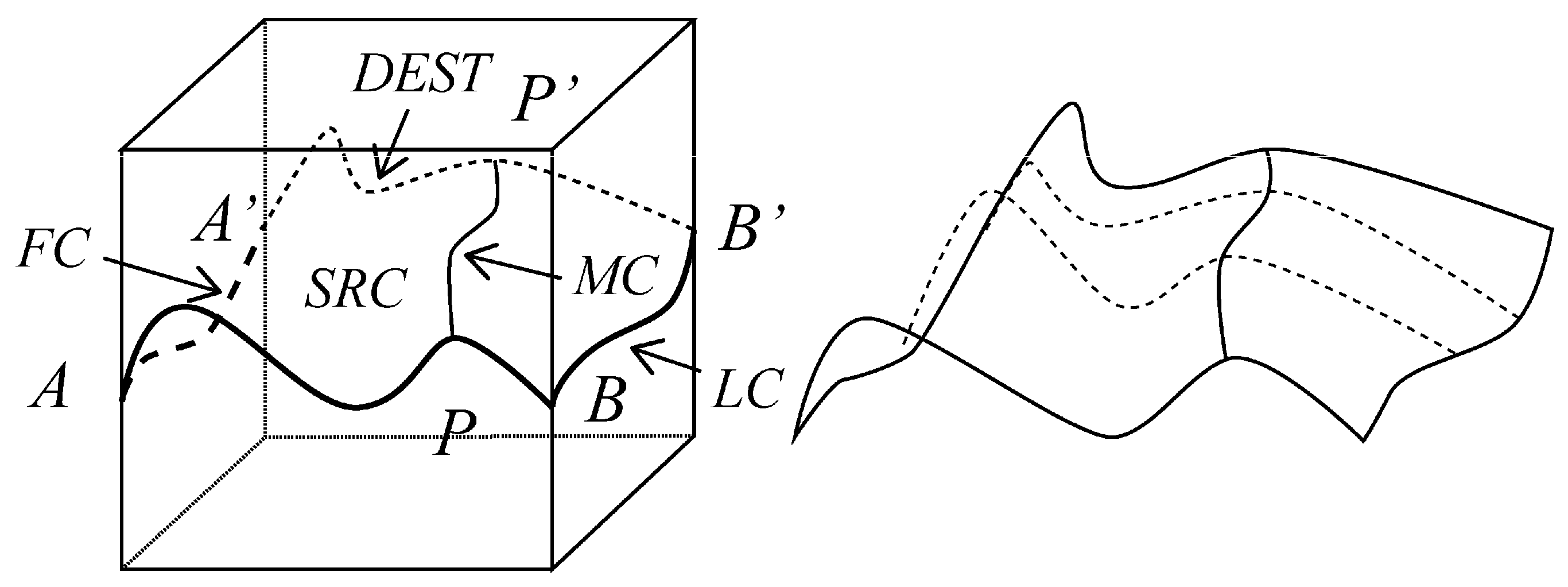
4.3. Interpolating the Mesh Surface of the Transverse Canyon Base on Morphing
- (1)
- Start boundary (SRC): interpolation start line—directed curve AB (A is the starting point).
- (2)
- Target boundary (DEST): end line of interpolation—directed curve A′B′ (A′ is the beginning point).
- (3)
- Constraint boundaries (MC, FC, LC): regulate the trend of transition curves such as AA′, BB′, and PP′ throughout the interpolation process. The first constraint (FC) is associated with the beginning point, while the final constraint (LC) is associated with the finishing position. The constraint positioned between FC and LC is known as the intermediate constraint (MC).
- (1)
- Constructing various sets of nodes. Separately saving the nodes on boundaries SRC, DEST, FC, and LC into ,, , and ,, , , and . Where , , , mean the index of each node, , , , are the number of nodes in each set and =, and ,, are the horizontal coordinate, longitudinal coordinate, and elevation of each node, respectively. In addition, , , ,and are the starting node of each line, and , , ,and are the ending node of each line.
- (2)
- Utilizing a contouring method to match nodes. A node in SRC may correlate to many nodes in DEST if . This study matches nodes using the Minimizing Span Length technique [74].
- (3)
- Constructing the transition curves. Suppose a transition curve TC exists, then the node set is , . Where represents the node’s index, and = if > ; = if ≤ . Using Equations (1) and (2), we can then determine the coordinate value of every node on TC.where Equation (1) calculates the unrestricted coordinates of the nodes on TC, and Equation (2) adjusts the elevation values of the nodes on TC. describes how close the TC is to the SRC and DEST. When = 0, the TC becomes the SRC. As increases, the TC moves away from SRC and closer to DEST. When = 1, the TC becomes DEST. Similarly, describes how close the is to the and .
- (4)
- Reconstructing the mesh surface. Saving each TC into , where is the index of TC, and is the number of TCs in TCS.
4.4. Generating the Paleotopographic DEM of the Transverse Canyon
- (1)
- Generating a DEM R_Dem via all mesh nodes using a spatial interpolation approach that is compatible with the input DEM. The extent of R_Dem is the same as the area of the transverse canyon, and the pixel is identical to the input DEM.
- (2)
4.5. Calculating Spatial Attributes of the Transverse Canyon
4.5.1. Surface Area
4.5.2. Volume
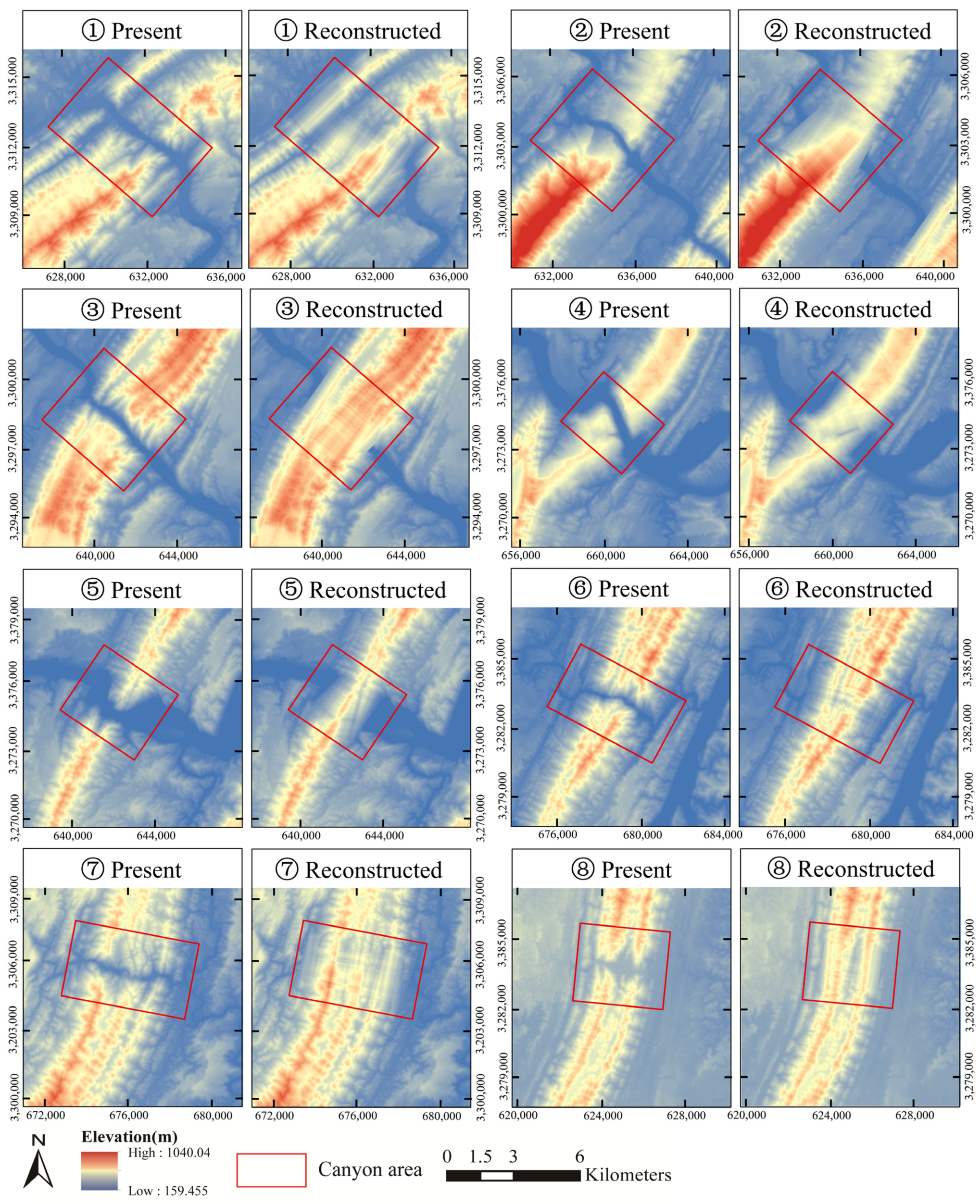
5. Results
6. Discussion and Applications
6.1. Factors Affecting the Method
6.1.1. Dislocated Mountains
6.1.2. Erosion Gullies
6.1.3. Different Types in Morphing
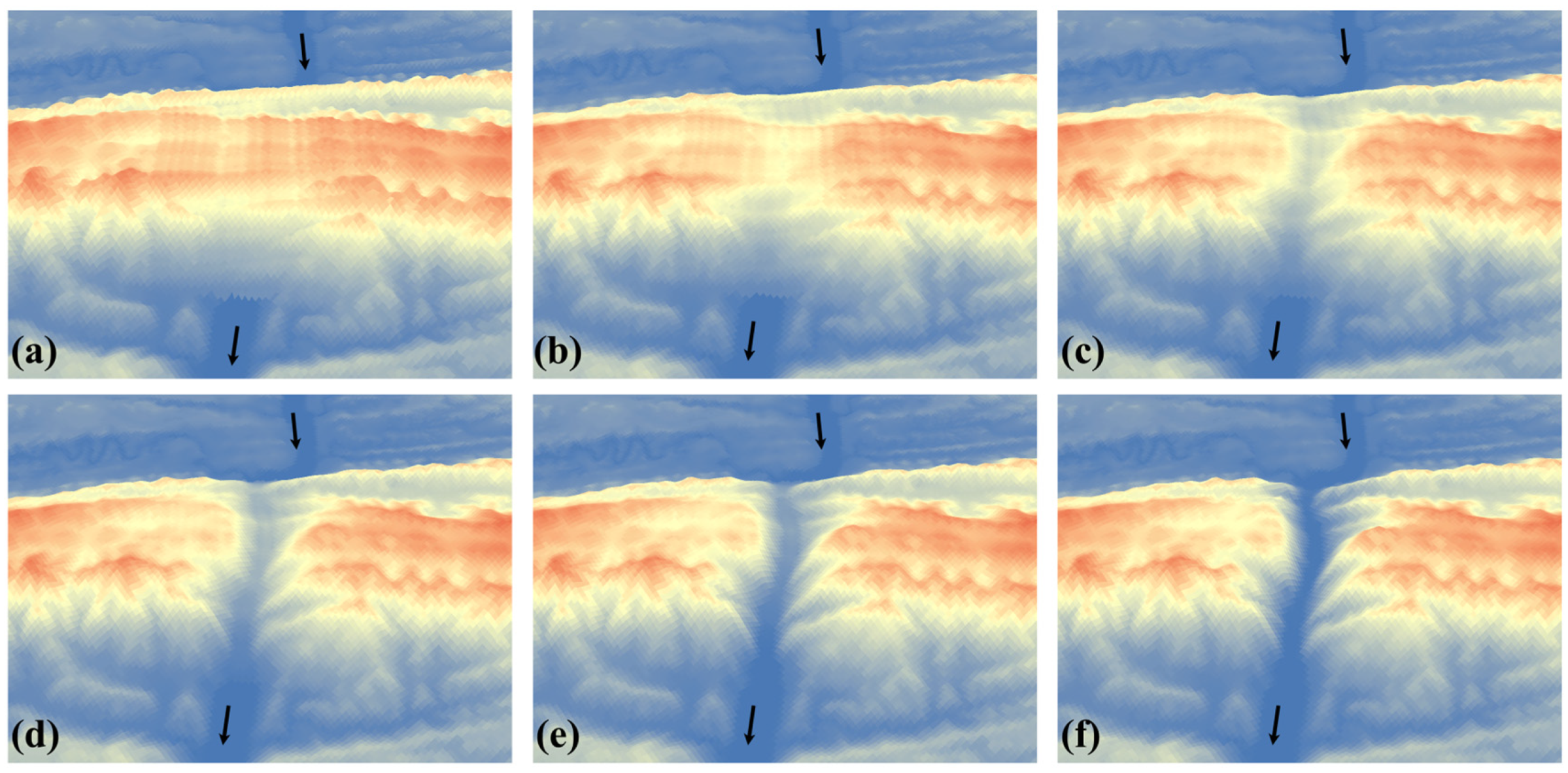
6.1.4. DEM “Jump”
6.2. Applicability of the Method for Other Secondary Valleys
6.3. Application Cases of the Reconstructed Paleotopography
6.3.1. Headward Erosion Simulation
6.3.2. Analysis of Paleodrainage Pattern
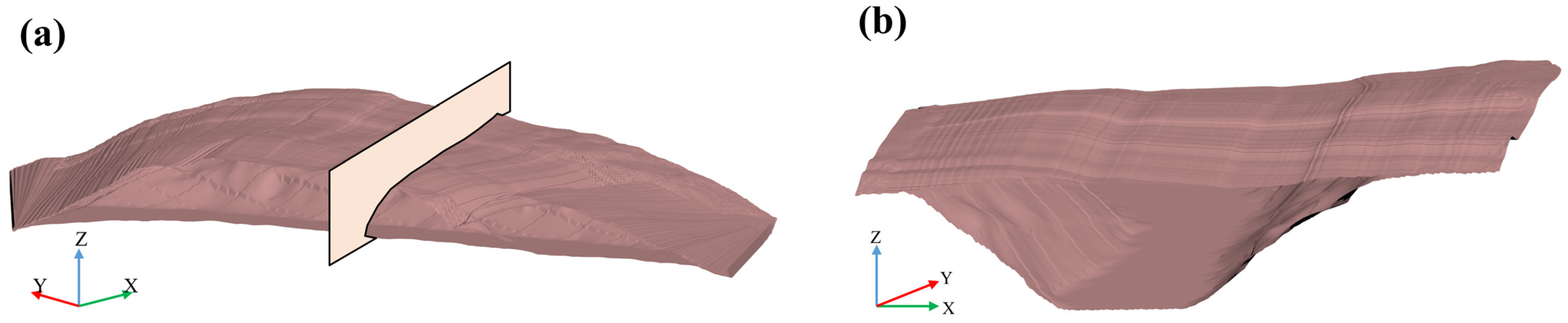
6.3.3. Three-Dimensional Model of the Transverse Canyon
6.4. Comparison between the Proposed Method and the Existing Methods
7. Conclusions
Author Contributions
Funding
Data Availability Statement
Conflicts of Interest
Computer Code and Software
References
- English, O. Oxford English Dictionary. In Encyclopedia of Swearing; Routledge: London, UK, 1976; p. 334. [Google Scholar]
- Yan, Q.; Iwasaki, T.; Stumpf, A.; Belmont, P.; Parker, G.; Kumar, P. Hydrogeomorphological Differentiation between Floodplains and Terraces. Earth Surf. Process. Landf. 2018, 43, 218–228. [Google Scholar] [CrossRef] [Green Version]
- Micallef, A.; Marchis, R.; Saadatkhan, N.; Clavera-Gispert, R.; Pondthai, P.; Everett, M.E.; Avram, A.; Timar-Gabor, A.; Cohen, D.; Trapani, R.P.; et al. Box Canyon Erosion along the Canterbury Coast (New Zealand): A Rapid and Episodic Process Controlled by Rainfall Intensity and Substrate Variability. Earth Surf. Dyn. 2020. [Google Scholar] [CrossRef]
- Ansari, S.; Rennie, C.D.; Venditti, J.G.; Kwoll, E.; Fairweather, K. Shore-Based Monitoring of Flow Dynamics in a Steep Bedrock Canyon River. E3S Web Conf. 2018, 40, 06025. [Google Scholar] [CrossRef] [Green Version]
- Cook, K.L.; Whipple, K.X.; Heimsath, A.M.; Hanks, T.C. Rapid Incision of the Colorado River in Glen Canyon–Insights from Channel Profiles, Local Incision Rates, and Modeling of Lithologic Controls. Earth Surf. Process. Landf. 2009, 34, 994–1010. [Google Scholar] [CrossRef]
- Glade, R.C.; Shobe, C.M.; Anderson, R.S.; Tucker, G.E. Canyon Shape and Erosion Dynamics Governed by Channel-Hillslope Feedbacks. Geology 2019, 47, 650–654. [Google Scholar] [CrossRef]
- Bracciali, L.; Najman, Y.; Parrish, R.R.; Akhter, S.H.; Millar, I. The Brahmaputra Tale of Tectonics and Erosion: Early Miocene River Capture in the Eastern Himalaya. Earth Planet. Sci. Lett. 2015, 415, 25–37. [Google Scholar] [CrossRef] [Green Version]
- Mitchell, N.C. Interpreting Long-Profiles of Canyons in the USA Atlantic Continental Slope. Mar. Geol. 2005, 214, 75–99. [Google Scholar] [CrossRef]
- Green, A.N.; Goff, J.A.; Uken, R. Geomorphological Evidence for Upslope Canyon-Forming Processes on the Northern KwaZulu-Natal Shelf, SW Indian Ocean, South Africa. Geo-Mar. Lett. 2007, 27, 399–409. [Google Scholar] [CrossRef]
- Reolid, J.; Bialik, O.M.; Puga-Bernabéu, Á.; Zilberman, E.; Cardenal, J.; Makovsky, Y. Evolution of a Miocene Canyon and Its Carbonate Fill in the Pre-Evaporitic Eastern Mediterranean. Facies 2022, 68, 6. [Google Scholar] [CrossRef]
- Schildgen, T.F.; Ehlers, T.A.; Whipp, D.M., Jr.; van Soest, M.C.; Whipple, K.X.; Hodges, K.V. Quantifying Canyon Incision and Andean Plateau Surface Uplift, Southwest Peru: A Thermochronometer and Numerical Modeling Approach. J. Geophys. Res.-Earth Surf. 2009, 114, F04014. [Google Scholar] [CrossRef]
- Wang, P.; Scherler, D.; Liu-Zeng, J.; Mey, J.; Avouac, J.-P.; Zhang, Y.; Shi, D. Tectonic Control of Yarlung Tsangpo Gorge Revealed by a Buried Canyon in Southern Tibet. Science 2014, 346, 978–981. [Google Scholar] [CrossRef] [PubMed] [Green Version]
- Maw, G. III.—Notes on the Comparative Structure of Surfaces Produced by Subaërial and Marine Denudation. Geol. Mag. 1866, 3, 439–451. [Google Scholar] [CrossRef] [Green Version]
- Gardner, J.V.; Armstrong, A.A.; Calder, B.R. Hatteras Transverse Canyon, Hatteras Outer Ridge and Environs of the U.S. Atlantic Margin: A View from Multibeam Bathymetry and Backscatter. Mar. Geol. 2016, 371, 18–32. [Google Scholar] [CrossRef] [Green Version]
- Hopkins, W.I. —On the Geological Structure of the Wealden District and of the Bas Boulonnais. Trans. Geol. Soc. Lond. 1845, 7, 1–51. [Google Scholar] [CrossRef] [Green Version]
- Thornbury, W.D. Principles of Geomorphology; John Wiley and Sons: New York, NY, USA, 1954; pp. 123–126. [Google Scholar]
- Larson, P.H.; Meek, N.; Douglass, J.; Dorn, R.I.; Seong, Y.B. How Rivers Get Across Mountains: Transverse Drainages. Ann. Am. Assoc. Geogr. 2017, 107, 274–283. [Google Scholar] [CrossRef]
- Douglass, J.; Schmeeckle, M. Analogue Modeling of Transverse Drainage Mechanisms. Geomorphology 2007, 84, 22–43. [Google Scholar] [CrossRef]
- Douglass, J.; Meek, N.; Dorn, R.I.; Schmeeckle, M.W. A Criteria-Based Methodology for Determining the Mechanism of Transverse Drainage Development, with Application to the Southwestern United States. Geol. Soc. Am. Bull. 2009, 121, 586–598. [Google Scholar] [CrossRef]
- Johnson, B. Stream Capture and the Geomorphic Evolution of the Linville Gorge in the Southern Appalachians, USA. Geomorphology 2020, 368, 107360. [Google Scholar] [CrossRef]
- Fan, N.; Kong, P.; Robl, J.C.; Zhou, H.; Wang, X.; Jin, Z.; Liu, X. Timing of River Capture in Major Yangtze River Tributaries: Insights from Sediment Provenance and Morphometric Indices. Geomorphology 2021, 392, 107915. [Google Scholar] [CrossRef]
- Pan, B.; Hu, Z.; Wang, J.; Vandenberghe, J.; Hu, X.; Wen, Y.; Li, Q.; Cao, B. The Approximate Age of the Planation Surface and the Incision of the Yellow River. Paleogeogr. Paleoclimatol. Paleoecol. 2012, 356, 54–61. [Google Scholar] [CrossRef]
- Cheng, S.; Deng, Q.; Zhou, S.; Yang, G. Strath Terraces of Jinshaan Canyon, Yellow River, and Quaternary Tectonic Movements of the Ordos Plateau, North China. Terra Nova 2002, 14, 215–224. [Google Scholar] [CrossRef]
- Hippolyte, J.-C.; Clauzon, G.; Suc, J.-P. Messinian-Zanclean Canyons in the Digne Nappe (Southwestern Alps): Tectonic Implications. Bull. Soc. Geol. Fr. 2011, 182, 111–132. [Google Scholar] [CrossRef] [Green Version]
- Yang, Z.; Shen, C.; Ratschbacher, L.; Enkelmann, E.; Jonckheere, R.; Wauschkuhn, B.; Dong, Y. Sichuan Basin and beyond: Eastward Foreland Growth of the Tibetan Plateau from an Integration of Late Cretaceous-Cenozoic Fission Track and (U-Th)/He Ages of the Eastern Tibetan Plateau, Qinling, and Daba Shan. J. Geophys. Res.-Solid Earth 2017, 122, 4712–4740. [Google Scholar] [CrossRef]
- Clark, M.K.; Schoenbohm, L.M.; Royden, L.H.; Whipple, K.X.; Burchfiel, B.C.; Zhang, X.; Tang, W.; Wang, E.; Chen, L. Surface Uplift, Tectonics, and Erosion of Eastern Tibet from Large-Scale Drainage Patterns. Tectonics 2004, 23, TC1006. [Google Scholar] [CrossRef] [Green Version]
- Clift, P.D.; Carter, A.; Wysocka, A.; Van Hoang, L.; Zheng, H.; Neubeck, N. A Late Eocene-Oligocene through-Flowing River between the Upper Yangtze and South China Sea. Geochem. Geophys. Geosyst. 2020, 21, e2020GC009046. [Google Scholar] [CrossRef]
- Alvarez, W. Drainage on Evolving Fold-Thrust Belts: A Study of Transverse Canyons in the Apennines. Basin Res. 1999, 11, 267–284. [Google Scholar] [CrossRef]
- Li, J.; Xie, S.; Kuang, M. Geomorphic Evolution of the Yangtze Gorges and the Time of Their Formation. Geomorphology 2001, 41, 125–135. [Google Scholar] [CrossRef]
- Darling, A.; Whipple, K. Geomorphic Constraints on the Age of the Western Grand Canyon. Geosphere 2015, 11, 958–976. [Google Scholar] [CrossRef] [Green Version]
- Ganjoo, R.K. The Vale of Kashmir: Landform Evolution and Processes. In Landscapes and landforms of India; Springer: Berlin/Heidelberg, Germany, 2014; pp. 125–133. [Google Scholar]
- Zheng, H.; Clift, P.D.; Wang, P.; Tada, R.; Jia, J.; He, M.; Jourdan, F. Pre-Miocene Birth of the Yangtze River. Proc. Natl. Acad. Sci. USA 2013, 110, 7556–7561. [Google Scholar] [CrossRef] [PubMed] [Green Version]
- Wang, X.; Bing, H.; Wu, Y.; Zhou, J.; Zhu, H.; Wu, Y.; Sun, H. Water Quality Variation and Its Conditioning Factors in the Three Gorges Reservoir, China. J. Water Clim. Chang. 2021, 12, 1694–1707. [Google Scholar] [CrossRef]
- Tao, Y.; Wang, Y.; Rhoads, B.; Wang, D.; Ni, L.; Wu, J. Quantifying the Impacts of the Three Gorges Reservoir on Water Temperature in the Middle Reach of the Yangtze River. J. Hydrol. 2020, 582, 124476. [Google Scholar] [CrossRef]
- Tang, M.; Xu, Q.; Huang, R. Site Monitoring of Suction and Temporary Pore Water Pressure in an Ancient Landslide in the Three Gorges Reservoir Area, China. Environ. Earth Sci. 2015, 73, 5601–5609. [Google Scholar] [CrossRef]
- Tang, H.; Wasowski, J.; Juang, C.H. Geohazards in the Three Gorges Reservoir Area, China–Lessons Learned from Decades of Research. Eng. Geol. 2019, 261, 105267. [Google Scholar] [CrossRef]
- Yu, T.; Liu, H.; Liu, B.; Tang, S.; Tang, Y.; Yin, C. Restoration of Karst Paleogeomorphology and Its Significance in Petroleum Geology—Using the Top of the Middle Triassic Leikoupo Formation in the Northwestern Sichuan Basin as an Example. J. Pet. Sci. Eng. 2022, 208, 109638. [Google Scholar] [CrossRef]
- Coleman, M.L.; Niemann, J.D.; Jacobs, E.P. Reconstruction of Hillslope and Valley Paleotopography by Application of a Geomorphic Model. Comput. Geosci. 2009, 35, 1776–1784. [Google Scholar] [CrossRef]
- Xiao, D.; Tan, X.; Fan, L.; Zhang, D.; Nie, W.; Niu, T.; Cao, J. Reconstructing Large-Scale Karst Paleogeomorphology at the Top of the Ordovician in the Ordos Basin, China: Control on Natural Gas Accumulation and Paleogeographic Implications. Energy Sci. Eng. 2019, 7, 3234–3254. [Google Scholar] [CrossRef] [Green Version]
- Lv, C.; Zhang, G.; Yao, Y.; Wu, S. Tectonic Evolution of the Wanan Basin, Southwestern South China Sea. Acta Geol. Sin. Engl. Ed. 2014, 88, 1120–1130. [Google Scholar] [CrossRef]
- Fu, X.Y.; Yang, Y.; Huang, Y.G.; Hao, L. Palaeomorphologic Reconstruction of Ordovician Karst in Southern Sulige Gasfield and Its Effect on Reservoir Distribution. Nat. Gas. Explor. Dev. 2014, 37, 1–4. (In Chinese) [Google Scholar]
- Wu, J.; Yang, H.; Xu, D. Introduction to the Recovery and Technology of Palaeogeomorphology in Sedimentary Basins. Adv. Mater. Res. 2015, 1073–1076, 2025–2030. [Google Scholar] [CrossRef]
- Sui, L.; Yang, W.; Song, B.; Wen, Q.; Sha, Z. Quantitative Restoration of Tongbomiao Formation Paleogeomorphology and Its Geological Significance in Tanan Depression. In Proceedings of the International Field Exploration and Development Conference, Xi’an, China, 16–18 October 2019; Springer: Berlin/Heidelberg, Germany, 2019; pp. 3309–3322. [Google Scholar] [CrossRef]
- Melo, A.H.; Magalhães, A.J.C.; Menegazzo, M.C.; Fragoso, D.G.C.; Florencio, C.P.; Lima-Filho, F.P. High-Resolution Sequence Stratigraphy Applied for the Improvement of Hydrocarbon Production and Reserves: A Case Study in Cretaceous Fluvial Deposits of the Potiguar Basin, Northeast Brazil. Mar. Pet. Geol. 2021, 130, 105124. [Google Scholar] [CrossRef]
- Hosseini, K.; Rezaee, P.; Kazem Shiroodi, S.; Moeini, M. Tectono-Sedimentary Evolution of the Maastrichtian Deposits in Western Part of Fars Area in a High Resolution Sequence Stratigraphic Framework. J. Pet. Res. 2021, 31, 146–153. [Google Scholar] [CrossRef]
- Huang, H.; Luo, Q. Mesozoic Group Denudation Recover and Its Petroleum Geologic Significations in the West Qaidam Basin. Pet. Explor. Dev. 2006, 33, 44. (In Chinese) [Google Scholar]
- Ding, R.; Chang, Y.; Min, K.; Xu, C.; Wang, W. Post-Orogenic Topographic Evolution of the Dabie Orogen, Eastern China: Insights from Apatite and Zircon (U-Th)/He Thermochronology. Geomorphology 2021, 374, 107487. [Google Scholar] [CrossRef]
- Braun, J.; Robert, X. Constraints on the Rate of Post-Orogenic Erosional Decay from Low-Temperature Thermochronological Data: Application to the Dabie Shan, China. Earth Surf. Process. Landf. 2005, 30, 1203–1225. [Google Scholar] [CrossRef]
- Wei, W.; Zuyi, Z. Reconstruction of Palaeotopography from Low-Temperature Thermochronological Data. Geol. Soc. Lond. Spec. Publ. 2009, 324, 99–110. [Google Scholar] [CrossRef]
- Jiao, R.; Yang, R.; Yuan, X. Incision History of the Three Gorges, Yangtze River Constrained From Inversion of River Profiles and Low-Temperature Thermochronological Data. J. Geophys. Res.-Earth Surf. 2021, 126, 2020JF005767. [Google Scholar] [CrossRef]
- Stokes, M.; Mather, A.E. Tectonic Origin and Evolution of a Transverse Drainage: The Río Almanzora, Betic Cordillera, Southeast Spain. Geomorphology 2003, 50, 59–81. [Google Scholar] [CrossRef]
- Harvey, A.M.; Wells, S.G. Response of Quaternary Fluvial Systems to Differential Epeirogenic Uplift: Aguas and Feos River Systems, Southeast Spain. Geology 1987, 15, 689–693. [Google Scholar] [CrossRef]
- Mayer, L.; Menichetti, M.; Nesci, O.; Savelli, D. Morphotectonic Approach to the Drainage Analysis in the North Marche Region, Central Italy. Quat. Int. 2003, 101, 157–167. [Google Scholar] [CrossRef]
- Wang, P.; Zheng, H.; Liu, S. Geomorphic Constraints on Middle Yangtze River Reversal in Eastern Sichuan Basin, China. J. Asian Earth Sci. 2013, 69, 70–85. [Google Scholar] [CrossRef]
- Aumann, G.; Ebner, H.; Tang, L. Automatic Derivation of Skeleton Lines from Digitized Contours. ISPRS-J. Photogramm. Remote Sens. 1991, 46, 259–268. [Google Scholar] [CrossRef]
- Jin, L.; Gao, X. Research on the Algorithm of Extracting Ridge and Valley Lines from Contour Data. Geo-Spat. Inf. Sci. 2005, 8, 282–286. [Google Scholar] [CrossRef] [Green Version]
- Chang, Y.-C.; Song, G.-S.; Hsu, S.-K. Automatic Extraction of Ridge and Valley Axes Using the Profile Recognition and Polygon-Breaking Algorithm. Comput. Geosci. 1998, 24, 83–93. [Google Scholar] [CrossRef]
- Liu, H.; Jin, H.; Miao, B. An Algorithm for Extracting Terrain Structure Lines Based on Contour Data. In Proceedings of the Sixth International Symposium on Digital Earth: Models, Algorithms, and Virtual Reality, Beijing, China, 9–12 September 2009; Volume 7840, pp. 286–291. [Google Scholar] [CrossRef]
- Strahler, A.N. Quantitative Analysis of Watershed Geomorphology. Eos Trans. Am. Geophys. Union 1957, 38, 913–920. [Google Scholar] [CrossRef] [Green Version]
- Martz, L.W.; Garbrecht, J. Numerical Definition of Drainage Network and Subcatchment Areas from Digital Elevation Models. Comput. Geosci. 1992, 18, 747–761. [Google Scholar] [CrossRef]
- Martz, L.W.; Garbrecht, J. An Outlet Breaching Algorithm for the Treatment of Closed Depressions in a Raster DEM. Comput. Geosci. 1999, 25, 835–844. [Google Scholar] [CrossRef]
- Jenson, S.K.; Domingue, J.O. Extracting Topographic Structure from Digital Elevation Data for Geographic Information System Analysis. Photogramm. Eng. Remote Sens. 1988, 54, 1593–1600. [Google Scholar]
- Zou, K.; Wo, Y.; Xu, X. A Feature Significance-Based Method to Extract Terrain Feature Lines. Geomat. Inf. Sci. Wuhan Univ. 2018, 43, 342–348. [Google Scholar] [CrossRef]
- Yan, S.; Tang, G.; Li, F.; Zhang, L. Snake Model for the Extraction of Loess Shoulder-Line from DEMs. J. Mt. Sci. 2014, 11, 1552–1559. [Google Scholar] [CrossRef]
- Zhu, H.; Tang, G.; Zhang, Y.; Yi, H.; Li, M. Thalweg in Loess Hill Area Based on DEM. Bull. Soil Water Conserv. 2003, 23, 43–45. [Google Scholar] [CrossRef]
- Zhou, Y.; Tang, G.; Wang, C.; Xiao, C.; Sun, J. A Novel Method for Automatic Extracting Loess Positive and Negative Terrains Based on Grid DEMs. In Proceedings of the 2009 First International Conference on Information Science and Engineering, Nanjing, China, 26–28 December 2009; pp. 3730–3732. [Google Scholar] [CrossRef]
- Lv, G.; Qian, Y.; Chen, Z. Study of automated extraction of shoulder line of valley from grid digital elevation data. Sci. Geogr. Sin. 1998, 18, 567–573. (In Chinese) [Google Scholar] [CrossRef]
- Yan, S.; Tang, G.; Li, F.; Dong, Y. An Edge Detection Based Method for Extraction of Loess Shoulder-Line from Grid DEM. Geomat. Inf. Sci. Wuhan Univ. 2011, 36, 363–367. (In Chinese) [Google Scholar] [CrossRef]
- Song, X.; Tang, G.; Li, F.; Jiang, L.; Zhou, Y.; Qian, K. Extraction of Loess Shoulder-Line Based on the Parallel GVF Snake Model in the Loess Hilly Area of China. Comput. Geosci. 2013, 52, 11–20. [Google Scholar] [CrossRef]
- Wang, Z.; Müller, J.-C. Line Generalization Based on Analysis of Shape Characteristics. Cartogr. Geogr. Inf. Sci. 1998, 25, 3–15. [Google Scholar] [CrossRef]
- Plazanet, C. Measurement, Characterization and Classification for Automated Line Feature Generalization. In Proceedings of the Autocarto-Conference; Citeseer: Princeton, NJ, USA, 1995; pp. 59–68. [Google Scholar]
- Seitz, S.M.; Dyer, C.R. View Morphing. In Proceedings of the 23rd Annual Conference on Computer Graphics and Interactive Techniques, New Orleans, LA, USA, 4–9 August 1996; pp. 21–30. [Google Scholar]
- Ming, J.; Yan, M. Three Dimensional Geological Surface Creation Based on Morphing. Geo-Spat. Inf. Sci. 2014, 30, 37–40. [Google Scholar] [CrossRef]
- Ekoule, A.B.; Peyrin, F.C.; Odet, C.L. A Triangulation Algorithm from Arbitrary Shaped Multiple Planar Contours. ACM Trans. Graph. 1991, 10, 182–199. [Google Scholar] [CrossRef]
- Papasaika, H.; Poli, D.; Baltsavias, E. Fusion of Digital Elevation Models from Various Data Sources. In Proceedings of the 2009 International Conference on Advanced Geographic Information Systems & Web Services, Cancun, Mexico, 1–7 February 2009; pp. 117–122. [Google Scholar]
- Fang, Q.; Zhu, W. On the features of canyon’s physical geography and its tourism value. Areal Res. Dev. 2002, 2, 68–71. [Google Scholar] [CrossRef]
- Xu, S.-Y.; Li, A.-B.; Dong, T.-T.; Xie, X.-L. Automatic Mapping of River Canyons Using a Digital Elevation Model and Vector River Data. Earth Sci. Inform. 2021, 14, 505–519. [Google Scholar] [CrossRef]
- Davis, W.M. A River-Pirate. Science 1889, 14, 108–109. [Google Scholar] [CrossRef] [Green Version]
- Yuan, T.; Lun, W.; Yong, G.; Daming, W.; Yi, Z. DEM-Based Modelling and Simulation of Modern Landform Evolution of Loess. In Advances in Digital Terrain Analysis; Springer: Berlin/Heidelberg, Germany, 2008; pp. 257–276. [Google Scholar] [CrossRef]
- Soille, P.; Gratin, C. An Efficient Algorithm for Drainage Network Extraction on DEMs. J. Vis. Commun. Image Represent. 1994, 5, 181–189. [Google Scholar] [CrossRef]
- Fox, M. A Linear Inverse Method to Reconstruct Paleo-Topography. Geomorphology 2019, 337, 151–164. [Google Scholar] [CrossRef]
- Clark, M.K. The Significance of Paleotopography. Rev. Mineral. Geochem. 2007, 66, 1–21. [Google Scholar] [CrossRef]


| Transverse Canyon | Length (km) | Depth (m) | Width (km) | Aspect Ratio | Plan-View Area (km2) | Surface Area (km2) | Volume (km3) |
|---|---|---|---|---|---|---|---|
| ➀ | 5.38 | 457.89 | 2.59 | 0.18 | 13.94 | 14.59 | 1.02 |
| ➁ | 3.39 | 632.80 | 3.30 | 0.19 | 11.09 | 11.44 | 0.91 |
| ➂ | 3.72 | 470.27 | 2.77 | 0.17 | 12.84 | 13.46 | 1.20 |
| ➃ | 2.75 | 352.20 | 1.66 | 0.21 | 3.74 | 3.97 | 0.37 |
| ➄ | 2.54 | 454.40 | 3.05 | 0.14 | 7.88 | 8.34 | 0.68 |
| ➅ | 3.88 | 454.33 | 2.14 | 0.21 | 7.55 | 8.13 | 0.46 |
| ➆ | 5.12 | 500.71 | 2.54 | 0.19 | 13.4 | 14.16 | 0.93 |
| ➇ | 2.79 | 266.99 | 1.68 | 0.15 | 5.75 | 6.1 | 0.31 |
Publisher’s Note: MDPI stays neutral with regard to jurisdictional claims in published maps and institutional affiliations. |
© 2022 by the authors. Licensee MDPI, Basel, Switzerland. This article is an open access article distributed under the terms and conditions of the Creative Commons Attribution (CC BY) license (https://creativecommons.org/licenses/by/4.0/).
Share and Cite
Shen, Y.; Li, A.; Xu, S.; Xie, X. A Morphing-Based Method for Paleotopographic Reconstruction of the Transverse Canyon. Remote Sens. 2022, 14, 6109. https://doi.org/10.3390/rs14236109
Shen Y, Li A, Xu S, Xie X. A Morphing-Based Method for Paleotopographic Reconstruction of the Transverse Canyon. Remote Sensing. 2022; 14(23):6109. https://doi.org/10.3390/rs14236109
Chicago/Turabian StyleShen, Yangen, Anbo Li, Shiyu Xu, and Xianli Xie. 2022. "A Morphing-Based Method for Paleotopographic Reconstruction of the Transverse Canyon" Remote Sensing 14, no. 23: 6109. https://doi.org/10.3390/rs14236109
APA StyleShen, Y., Li, A., Xu, S., & Xie, X. (2022). A Morphing-Based Method for Paleotopographic Reconstruction of the Transverse Canyon. Remote Sensing, 14(23), 6109. https://doi.org/10.3390/rs14236109