Improved LiDAR Localization Method for Mobile Robots Based on Multi-Sensing

Abstract

In this paper, we propose a localization method applicable to 3D LiDAR by improving the LiDAR localization algorithm, such as AMCL (Adaptive Monte Carlo Localization). The method utilizes multiple sensing information, including 3D LiDAR, IMU and the odometer, and can be used without GNSS. Firstly, the wheel speed odometer and IMU data of the mobile robot are multi-source fused by EKF (Extended Kalman Filter), and the sensor data obtained after multi-source fusion are used as the motion model to participate in the positional prediction of the particle set in AMCL to obtain the initial positioning information of the mobile robot. Then, the position pose difference values output by AMCL at adjacent moments are substituted into the PL-ICP algorithm as the initial position pose transformation matrix, and the 3D laser point cloud is aligned with the nonlinear system using the PL-ICP algorithm. The three-dimensional laser odometer is obtained by LM (Levenberg--Marquard) iterative solution in the PL-ICP algorithm. Finally, the initial position pose output by AMCL is corrected by the three-dimensional laser odometer, and the AMCL particles are weighted and sampled to output the final positioning result of the mobile robot. Through simulation and practical experiments, it is verified that the improved AMCL algorithm has higher positioning accuracy and stability compared to the AMCL algorithm.

1. Introduction

Mobile robot positioning is a state estimation problem of the mobile robot’s own position $(x,y)$ and yaw angle $\theta$ [1] and is also the basis for the autonomous navigation of the mobile robot. Localization information about the mobile robot should be as accurate as possible to provide reliable position estimation for subsequent path planning and navigation control. Efficient and accurate positioning information facilitates the mobile robot to quickly and reasonably plan the movement route so that the mobile robot body can precisely reach the designated position for the task operation.

Currently, the most widely used and computationally efficient mobile robot localization method in the industry is AMCL (Adaptive Monte Carlo Localization) [2], which is a localization method derived from improved optimization based on the MCL (Monte Carlo Localization) [3]. The AMCL algorithm takes the motion model of the mobile robot and the observation model of the LiDAR (Laser Radar) as input quantities and obtains the global positional information of the mobile robot in the navigational coordinate system through the probabilistic model of particle filtering with high computational efficiency and good real-time performance. The AMCL algorithm has now become the only specified localization algorithm in the ROS (Robot Operating System) Navigation Stack for mobile robots. Although the AMCL localization algorithm has become mature, the main hardware selection of the AMCL algorithm is 2D LiDAR. Combining mainstream research status and methods, we optimize and improve the AMCL algorithm based on multi-sensing information to make it more suitable for 3D LiDAR localization research and improve the localization accuracy and stability of the AMCL algorithm.

With the continuous development of SLAM methods in the last decade, SLAM (Simultaneous Localization and Mapping) methods are divided into laser SLAM and vision SLAM according to the type of sensors used [4]. Laser SLAM uses LiDAR as an external sensor for environment measurement [5], and vision SLAM relies on cameras for environment perception [6]. Currently, 3D LiDAR demonstrates better adaptability and greater robustness compared to 2D LiDAR and cameras [7], both indoors and outdoors. On the one hand, 3D LiDAR can measure the environment directly [8,9,10], and the amount of acquired point cloud data is much larger than 2D LiDAR, which has better reliability and higher data accuracy. On the other hand, 3D LiDAR is not affected by light intensity, which has better stability and lower calculation complexity compared with cameras in the process of use. Maps constructed by SLAM are usually classified as 3D sparse maps, 3D dense maps and 2D occupied maps, where 3D sparse maps are suitable for mobile robot localization studies, 3D dense maps are suitable for mobile robots to model the environment for perception, and 2D occupied maps are suitable for planar navigation of mobile robots. In the study of planar navigation method for mobile robots, 3D LiDAR is selected not only to build a 3D environment point cloud map but also to generate a 2D occupied raster map suitable for planar navigation of mobile robots, and the 3D point cloud can be data converted to 2D point cloud according to the format requirements so that 3D LiDAR can be used as high quality and high precision 2D LiDAR, which has good scalability and research value.

Because the AMCL algorithm requires the input of a 2D laser point cloud, it needs to process the point cloud data of 3D LiDAR, based on which a simple and efficient point cloud conversion method is proposed in this paper. In addition, the AMCL algorithm uses the mobile robot motion model for localization, and the mobile robot motion model involves the wheel speed odometer model. The odometer has accumulated errors during the robot motion, resulting in the limited positional accuracy output by the AMCL algorithm, which reduces the localization accuracy of the mobile robot. To improve the problem of low initial accuracy of the odometer of mobile robots, researchers usually choose to fuse the odometer data of mobile robots with other sensor data and use the fused sensor data as the motion model of the AMCL algorithm for mobile robot localization studies. Currently, the most commonly used sensor is IMU because IMU (Inertial Measurement Unit) is cheaper compared to GNSS (Global Navigation Satellite System) receivers and is easy to be used, not affected by signal interference and more versatile [11]. However, IMU yaw angle measurement for mobile robots generates cumulative errors as time grows, resulting in the output accuracy of yaw angle and overall positioning stability of the AMCL algorithm not being guaranteed. Given that the fusion of IMU and wheel speed odometer of the mobile robot can obtain more accurate odometer information, and the high-precision three-dimensional laser odometer obtained by 3D LiDAR has a more accurate yaw angle [12,13,14], which can compensate for the unreliability of the IMU yaw angle. The multi-sensing localization method based on 3D LiDAR, IMU and wheel speed odometer is a mobile robot localization scheme with complementary sensing information and high reliability. In this paper, the AMCL algorithm is optimized and improved based on 3D LiDAR, IMU and odometer information to improve the output accuracy and positioning stability of the AMCL algorithm. The methodological framework studied in this paper is shown in Figure 1.

2. Related Work

2.1. AMCL-Based Multi-Sensing Fusion Localization Method

Since sensors are inevitably affected by noise during the measurement, AMCL positioning studies using a single sensor data in a positioning system are prone to problems such as low positioning accuracy and positioning failure. In recent years, researchers have improved the localization accuracy of the AMCL algorithm by using a multi-sensor fusion scheme based on the AMCL algorithm. In the study [15], de Miguel M Ál fused the use of 3D LiDAR information and GNSS information based on the AMCL algorithm to improve the localization accuracy of mobile robots in outdoor environments while solving the abduction problem of mobile robots. In the study [16], Liu Yanjie used neural networks to fuse vision and 2D laser rangefinder data based on the AMCL algorithm to improve the accuracy and precision of mobile robots for repositioning in indoor scenes. In the study [17], G Ge proposed the Text-MCl localization method based on the AMCL algorithm by using environmental semantic information and LiDAR scanning information to improve the speed and success rate of global localization of mobile robots. In the study [18], Obregón D fused GNSS, mobile robot chassis odometer data, used fused sensor data as prediction data for the AMCL algorithm, and verified the effectiveness and robustness of the improved AMCL localization method through experiments. In the study [19], AA Fikri systematically integrated the AMCL algorithm with the Google cartographer mapping method by fusing mobile robot odometer and IMU data through the eulerdometer method to reduce systematic errors in the mapping and localization process of mobile robots. In the study [20], Portugal D improved the robustness of a continuous localization system for mobile robots based on the AMCL algorithm, sensor data fusion and scan matching techniques. The above-mentioned studies have achieved certain results, but there are still certain shortcomings. For example, the applicability of some research methods is reduced when GNSS signals are missing, and some other research methods only improve the localization error of the AMCL algorithm in the linear direction, and the yaw angle error is larger, which in general leads to the poor stability of AMCL algorithm. In special scenarios, such as indoor and outdoor substations and coal-chemical plants, GNSS cannot be used for satellite positioning, and the low positioning accuracy of LiDAR alone cannot guarantee the safety of robot operations. To address such problems, this paper conducts a study to improve the positioning accuracy of LiDAR in special scenarios by using the advantages of complementary sensing to enhance the safety of robot operations. In this paper, based on the improved AMCL algorithm, which incorporates IMU and an odometer, we added a three-dimensional laser odometer to correct the initial AMCL positioning results, continuing to improve the positioning accuracy and stability of the AMCL algorithm.

2.2. Multi-Source Data Fusion Method

Sensor fusion system is a complex information system, and various sensors collect information in real-time, with continuity and timing characteristics of each, and there are also mutual constraints and influence between various information [21]. Multi-source data fusion methods are the key and core of multi-sensor data fusion and localization methods [22]. At present, multi-source data fusion methods are mainly divided into four categories: inference methods [23], classification methods [24], artificial intelligence methods [25] and filter estimation methods [26]. The inference methods are mainly based on D-S evidence theory, which provides a good solution to deal with the ambiguity and uncertainty of sensor information and is now widely used in the fields of image processing and target recognition [27]. The common clustering and fusion algorithm used in classification methods are K-means, which is based on the Euclidean distance to judge the target data, and the closer the target data is, the higher the similarity of the target data is so that the data with greater similarity are gathered and fused together to achieve classification [28]. The artificial intelligence methods are mainly based on artificial neural networks for the fusion of multi-source data information, and artificial neural networks assign network weights through learning algorithms while reasoning about the uncertainty of multi-sensing data and then use the signal processing capability and automatic reasoning function of neural networks to achieve data fusion [29]. The filter estimation method has become the most widely used and researched method due to its better robustness and applicability in dynamic and complex states, and a typical representative method is the Kalman Filter algorithm [30]. The Kalman Filter algorithm, first proposed by Hungarian mathematician Rudolf Emil Kalman [31], can achieve optimal estimation for linear systems, but the traditional Kalman filter algorithm is only applicable to linear Gaussian systems, especially when the system state information and observation information are linear functions. For mobile robot positioning, the system is in a nonlinear state most of the time, and the Kalman filter method for data fusion has certain drawbacks: on the one hand, the state equation and observation information of the system is inaccurate, and the difference between the actual observed and estimated values is too large. On the other hand, as the amount of observations increases in the calculation process, the cumulative error generated by the calculation gradually becomes larger, the error covariance matrix gradually loses its positive character, and the trade-off effect of Kalman gain fails. In this case, two nonlinear Kalman filtering methods are generated [32,33]: UKF (Unscented Kalman Filter) and EKF (Extended Kalman Filter). UKF was proposed by S. Julier, and a new method was generated by combining UT and KF (Kalman Filter) [34,35]. The essence of the method is to estimate the system state variables by using the framework of the Kalman filter algorithm after obtaining an approximately linear system through UT transformation, but the lossless transformation is influenced by noise in practical applications, and the system stability needs to be improved. Compared with UKF, the EKF proposed by Bucy and Y. Sunahara et al. has stronger applicability in mobile robot localization studies [36,37], using Taylor series expansion to linearize the nonlinear function segments and filter them through the framework of the Kalman filter algorithm to complete the optimal estimation of the state of the target with high data fusion accuracy and good stability. In this paper, the fusion of the mobile robot odometer and IMU data is performed precisely based on the EKF algorithm framework [38].

2.3. Point Cloud Registration

The 3D LiDAR has high accuracy and reliability. The 3D laser point cloud is aligned to obtain a high-accuracy three-dimensional laser odometer, and the three-dimensional laser odometer can accurately estimate the movement of the LiDAR in a short period of time. Currently, the common methods for aligning laser point clouds are the ICP (Iterative Closest Point, ICP) algorithm [39] and the NDT (Normal Distribution Transformation, NDT) algorithm [40], but the common method for finding the exact transformation relationship between two LiDAR scans is ICP. The ICP algorithm aligns two point sets by finding the closest relationship point by point until the convergence condition is satisfied and stops iterating, but when the point set sample size is large, the ICP algorithm may be very computationally resource-intensive [41]. To address this problem, researchers have improved ICP algorithms and proposed new algorithms, such as the GICP (Generalized-ICP, GICP) algorithm [42], which achieves local plane alignment by matching two scans. NICP (Normal ICP, NICP) algorithm [43] requires the same direction of the normal vector in the plane where the point cloud is located when aligning the point cloud and considers the angular difference of the normal vectors of the corresponding points in addition to the Euclidean distance of the corresponding points when calculating the alignment error of the point cloud. In recent years, some variants of ICP algorithms have been proposed to improve the accuracy and operational efficiency of ICP algorithms [44,45]. The PL-ICP (Point-to-Line ICP) algorithm used in this paper is one of them, which iteratively matches the laser point cloud based on the distance from a point to a line, and each scan is a sampling of a plane of the physical world, which is more suitable for non-linear scenarios in the localization of mobile robots. In this paper, an interaction design between the PL-ICP algorithm and the AMCL algorithm is performed. The initial positioning information from AMCL provides the initial positional matrix for the PL-ICP algorithm, and then the three-dimensional laser odometer between laser point cloud frames calculated by PL-ICP is used as feedback information to correct the initial positioning information from AMCL.

3. Principles and Models

3.1. AMCL and Laser Point Cloud Data Conversion

3.1.1. AMCL

The AMCL algorithm is superior to the MCL algorithm and is widely chosen as the LiDAR probabilistic localization method on mobile robots for localization use. Specifically, it was implemented using a form of ROS nodes, as the algorithm is a stable and maintained version. Most of the parameters of the algorithm are set to default values, where the odometer is selected as the differential model, the laser model is the likelihood field, the maximum number of particles is 5000, and the minimum number of particles is 500. The odometer model defines the equations of motion to better describe the differential motion of the mobile robot, and the laser model describes the probabilistic method used to calculate the probability that the mobile robot is at a certain position given a certain laser measurement; the maximum and minimum particles represent the maximum and minimum possible positions around the mobile robot, respectively.

3.1.2. Laser Point Cloud Data Conversion

In this paper, we use Velodyne 16-line LiDAR for LiDAR hardware selection, and the AMCL localization algorithm needs to rotate the 2D LiDAR to obtain the surrounding environment information about the mobile robot and match with the prior map data to realize the localization function of the mobile robot; therefore, we designed a 3D point cloud data conversion method. After the Velodyne 16-line LiDAR starts working, the LiDAR point cloud data conversion method proposed in this paper is run, and the converted laser point cloud data is passed to the AMCL algorithm as an input quantity.

Taking Velodyne 16-line LiDAR as an example, the laser point cloud data conversion process proposed in this paper mainly includes: first, we calculate the horizontal angle and distance data statistics for the point cloud data points acquired by Velodyne 16-line LiDAR, and then we reserve the points with the same horizontal angle among the 16 laser beams and the closest to the LiDAR origin position, while the LiDAR needs to be installed at a higher position from the ground on the mobile robot body in order to avoid the large interference caused by the ground point cloud.

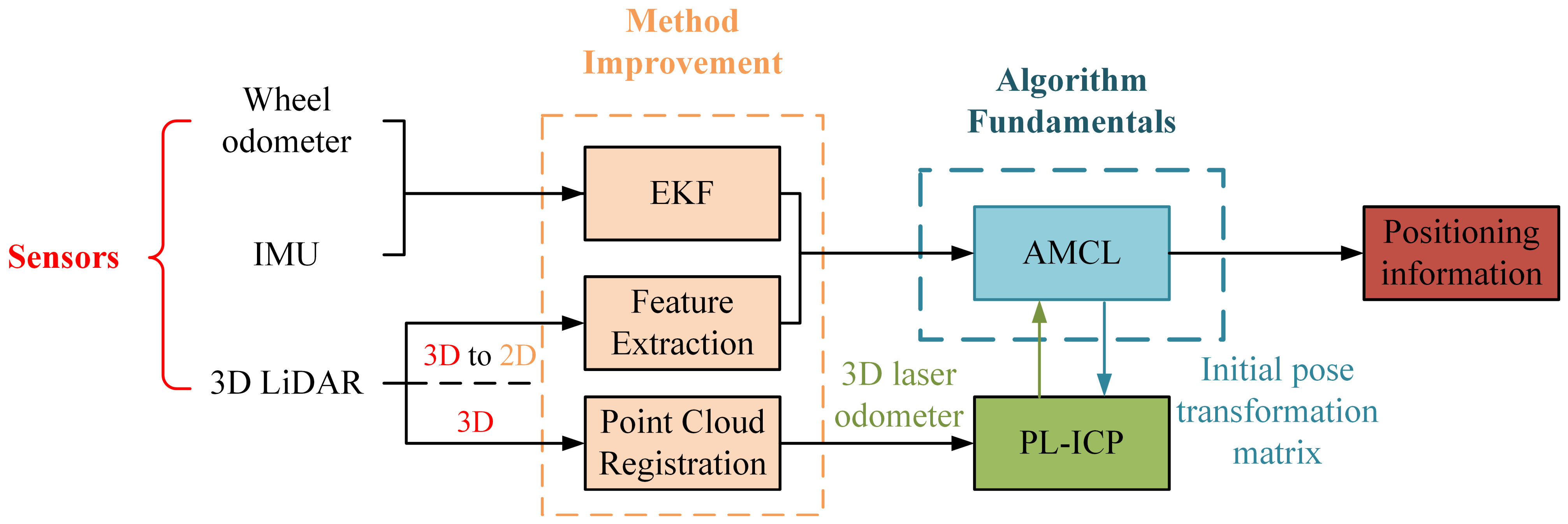
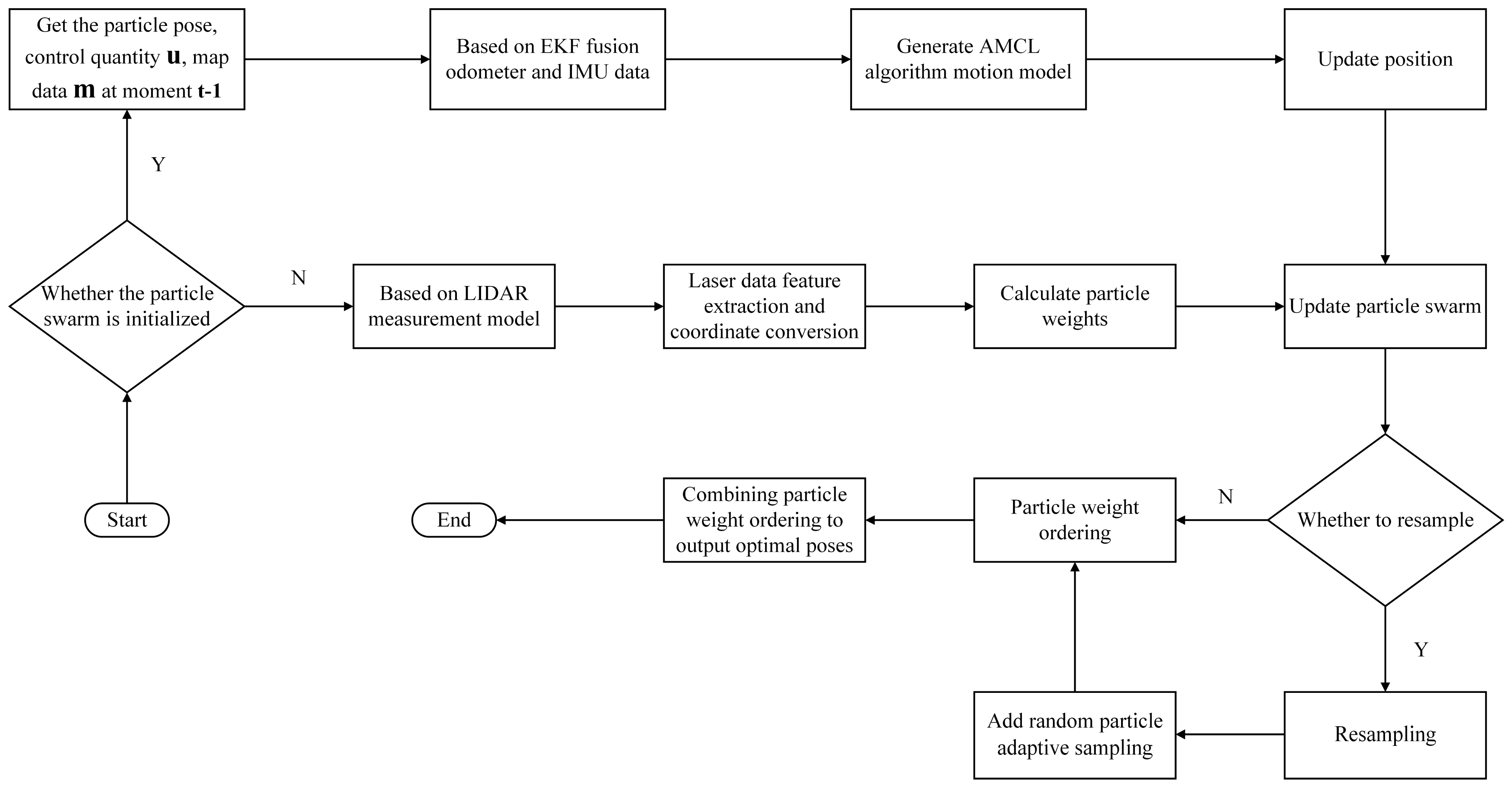
3.2. Improved AMCL Localization Algorithm Based on EKF Fusion

The overall flow of the improved AMCL algorithm based on EKF fusion is shown in Figure 2. The overall process mainly includes particle set initialization, particle swarm update, particle weight calculation and resampling.

The odometer data of the mobile robot’s wheel speed, the particle’s attitude at $t-1$ and the control volume $u_{t-1}$ are obtained, and the estimated particle’s attitude at $t$ is obtained by the fusion model of the EKF-based odometer and IMU, and the whole particle swarm is updated. The control quantity $u_t=(a_x,a_y,w)$ at time $t$, where $a_x$ is the acceleration of the mobile robot in the $X$-axis direction, $a_y$ is the acceleration of the mobile robot in the $Y$-axis direction, and $w$ is the angular velocity of the mobile robot rotating around axis $Z$. The estimated poses of the odometer and IMU at time $t-1$ and $t$ after the EKF filtered fusion are expressed as:

$$X_{m,t-1}={\left(x_{m,t-1},y_{m,t-1},{\theta }_{m,t-1}\right)}^T$$

(1)

$$X_{m,t}={\left(x_{m,t},y_{m,t},{\theta }_{m,t}\right)}^T$$

(2)

The attitude of the particle at the moment of time $t-1$ is expressed as:

$$X_{t-1}={\left(x_{t-1},y_{t-1},{\theta }_{t-1}\right)}^T$$

(3)

Sampling from the difference between the estimated poses at moments $t-1$ and $t$ and the amount of positional change of the mobile robot at the moment of time can be obtained as:

$$\Delta \theta =atan2\left(y_{m,t}-y_{m,t-1},x_{m,t}-x_{m,t-1}\right)-{\theta }_{m,t-1}$$

(4)

$$\Delta S=\sqrt{{\left(x_{m,t}-x_{m,t-1}\right)}^2+{\left(y_{m,t}-y_{m,t-1}\right)}^2}$$

(5)

where $atan2(a,b)$ is the arctangent function.

Adding sampling error $sample\left({\sigma }^2\right)$ to $\Delta \theta$ and $\Delta S$ respectively, the change in the mobile robot’s positional change after adding sampling error is expressed as:

$$\Delta \theta =\Delta \theta +sample\left({\alpha }_1\Delta S^2+{\alpha }_1\Delta {\theta }^2\right)$$

(6)

$$\Delta S=\Delta S+sample\left({\alpha }_3\Delta S^2+{\alpha }_4\Delta {\theta }^2\right)$$

(7)

$$\gamma =sample\left({\alpha }_5\Delta S^2+{\alpha }_6\Delta {\theta }^2\right)$$

(8)

In the above equation: $\gamma$ is an additional random disturbance, ${\alpha }_1,{\alpha }_2,\dots ,{\alpha }_6$ is the motion noise parameter and $sample\left({\sigma }^2\right)$ is a random sample with a Gaussian distribution with mean $0$ and variance ${\sigma }^2$.

The final corrected particle positional representation at moment $t$ can be obtained as $X_t={\left(x_t,y_t,{\theta }_t\right)}^T$.

$$\left\{\begin{array}{c}{x}_t=x_{t-1}-\Delta Ssin\theta +\Delta Ssin\left(\theta +\Delta \theta \right)\\ y_t=y_{t-1}+\Delta Scos\theta -\Delta Scos\left(\theta +\Delta \theta \right)\\ {\theta }_t={\theta }_{t-1}+\Delta \theta +\gamma \Delta t\end{array}\right.$$

(9)

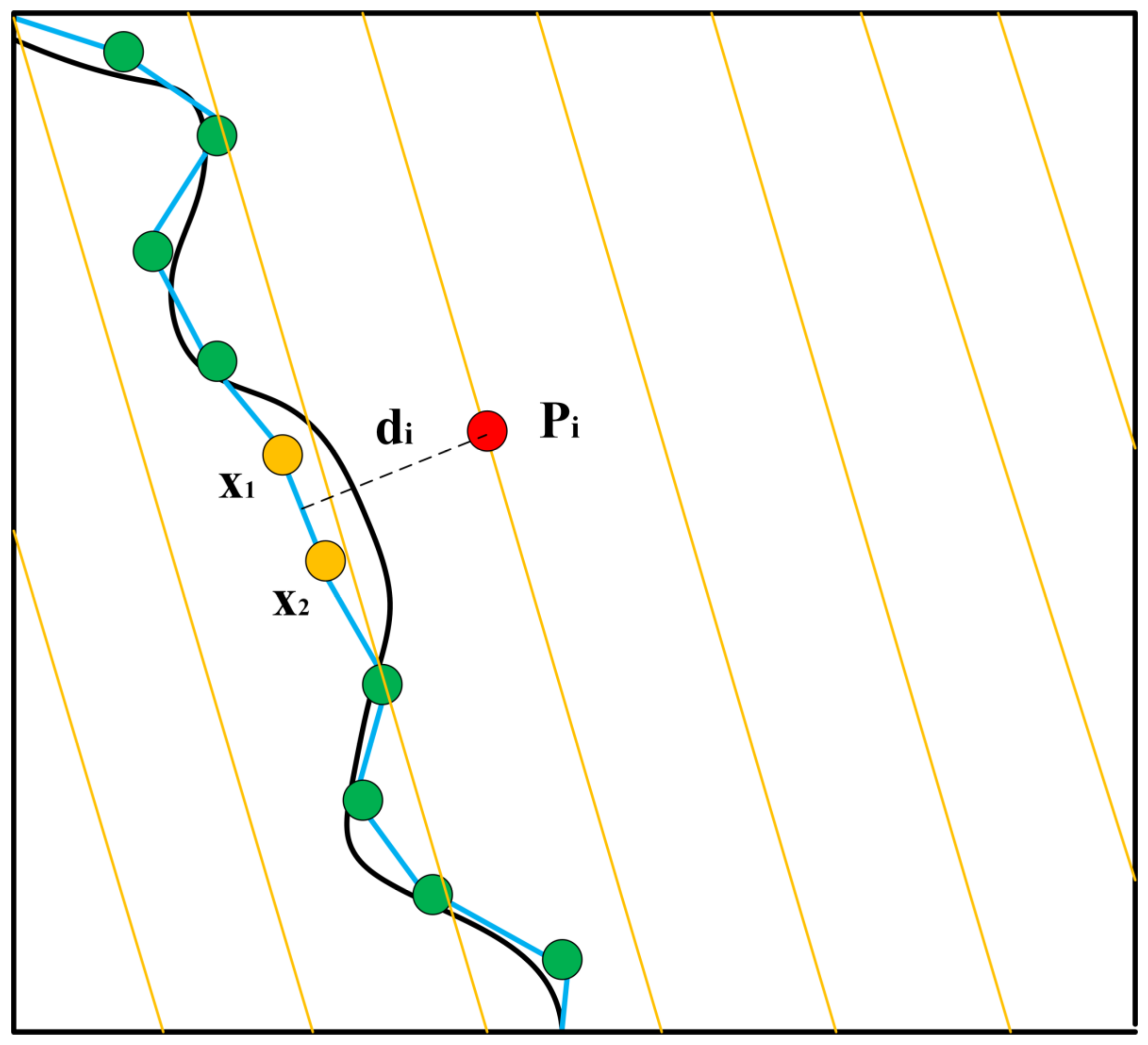
3.3. PL-ICP Point Cloud Matching Correction Based on the Improved AMCL

The PL-ICP algorithm optimizes the point cloud matching iteratively by linearizing the environmental surface segments using the distance of the line from the laser point cloud in the current frame to the two closest points in the previous frame, as shown in Figure 3.

The main process of the PL-ICP algorithm is as follows: firstly, find the two closest points in the previous point cloud $X$ based on any point $p_i$ in the current point cloud $P$, which are recorded as $x_1$ and $x_2$, respectively, and then calculate the distance $d_i$ from point $p_i$ to the line where points $x_1$ and $x_2$ are located until convergence. However, the PL-ICP algorithm is more sensitive to the initial value, and a good initial value will make the point cloud alignment results more accurate, while on the contrary, the point cloud alignment error is larger. Therefore, in this paper, based on AMCL multi-sensing fusion, we use multi-sensing information fusion to provide more accurate localization initial values to compensate for this deficiency of the PL-ICP algorithm, and the error equation of PL-ICP algorithm is shown in Equation (10).

$$E\left(R,T\right)={\displaystyle \sum _i{\left(n_i^T\left[R\left({\theta }_t\right)p_i+T_t-x_i\right]\right)}^2}$$

(10)

where $n_i^T$ is the unit normal vector perpendicular to the line where points $x_1$ and $x_2$ are located, $R$ is the point cloud rotation matrix and $T$ is the point cloud translation matrix. The current frame of the laser point cloud $P$ is rotated and translated by $\left(R,T\right)$ to obtain a new point cloud set $\overline{P}$ and then iterated. When $E\left(R,T\right)$ is less than the set threshold or the number of iterations meets the requirement, the iteration is stopped and the final result $\left(R,T\right)$ is output to obtain the relative position difference of the two laser point cloud frames. The poses of the mobile robot corrected by fusion-improved AMCL at moments $t-1$ and $t$ are known to be:

$$\stackrel{\wedge }{X_{t-1}}={\left(x_{AMCL,t-1},y_{AMCL,t-1},{\theta }_{AMCL,t-1}\right)}^T$$

(11)

$$\stackrel{\wedge }{X_t}={\left(x_{AMCL,t},y_{AMCL,t},{\theta }_{AMCL,t}\right)}^T$$

(12)

The initial values $\left(R_0,T_0\right)$ of the rotation and translation matrix iterations in the PL-ICP algorithm are obtained from the difference of the mobile robot poses at moments $t-1$ and $t$ output by AMCL. Converting the laser point cloud set $P$ at moment $t$ to the point cloud set $X$ at moment $t-1$ in the coordinate system, the error distance is expressed as:

$$e_i=n_i^T\left[R\left({\theta }_T\right)p_i+T_t-x_i\right]$$

(13)

The error function is solved iteratively using the LM method, and finally, $\left(R,T\right)$ minimizes the error $E\left(R,T\right)$. The bitwise transformation in the translation matrix $T$ and the rotation matrix $R$ are expressed as:

$$T={\left[T_x,T_y\right]}^T$$

(14)

$$R=\left[\begin{array}{cc}cos{\theta }_R& -sin{\theta }_R\\ sin{\theta }_R& cos{\theta }_R\end{array}\right]$$

(15)

Solving for the rotation angle ${\theta }_R$ yields:

$${\theta }_R=atan2(cos{\theta }_R,sin{\theta }_R)$$

(16)

The rotation angle ${\theta }_R$ is in the range of $\left(-\pi ,\pi \right)$. The final position $X_{p,t}$ of the mobile robot after PL-ICP point cloud matching at the moment of $t$ correction is expressed as:

$$X_{p,t}=\left[\begin{array}{c}{x}_{p,t}\\ y_{p,t}\\ {\theta }_{p,t}\end{array}\right]=\left[\begin{array}{c}{x}_{p,t-1}\\ y_{p,t-1}\\ {\theta }_{p,t-1}\end{array}\right]+\left[\begin{array}{ccc}cos{\theta }_{p,t-1}& -sin{\theta }_{p,t-1}& 0\\ sin{\theta }_{p,t-1}& cos{\theta }_{p,t-1}& 0\\ 0& 0& 1\end{array}\right]\left[\begin{array}{c}{T}_x\\ T_y\\ {\theta }_R\end{array}\right]$$

(17)

4. Results and Analyses

Two different sets of experiments were carried out. On the one hand, the proposed approach is to test using simulation scenarios to obtain qualitative results. On the other hand, the positioning study of the mobile robot was performed by relying on the experimental platform to obtain quantitative and practical results. The experimental platform of this paper includes a computer with an i5-11400 processor and NVIDIA GTX1650s graphics card, and the computer uses Ubuntu 18.04 melodic version and Robot Operating System (ROS). All algorithms are implemented based on C++.

4.1. Simulation Experiments

4.1.1. Simulation Environment

We built a simulation environment through Gazebo software and established a mobile robot model using xacro files, as shown in Figure 4.

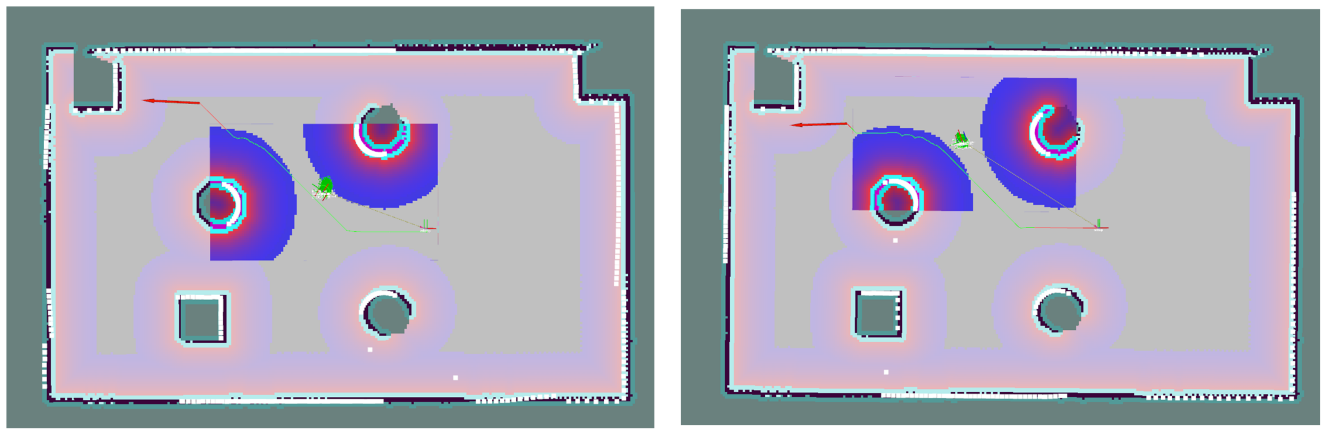
4.1.2. Point Cloud Matching Correction for AMCL Positioning

PL-ICP point cloud matching is the last part of the positioning system designed in this paper, which directly corrects the AMCL positioning results based on the improved fused IMU and odometer. In order to verify the effect of a three-dimensional laser odometer on AMCL algorithm positional correction, the laser point cloud data is converted from under the lidar coordinate system to the coordinate navigation system in the ROS upper navigation system, the PL-ICP algorithm is run, and the improved AMCL positioning information is read, the original laser point cloud data topic and the PL-ICP corrected point cloud topic are subscribed respectively, and the 2D raster laser point cloud map before and after the point cloud correction is obtained, as shown in Figure 5.

As can be seen in Figure 5, before the three-dimensional laser odometer correction of the AMCL localization results, there are some areas where the laser point cloud does not overlap with the map, indicating a bias in the mobile robot’s position estimation before correction. After the three-dimensional laser odometer correction, the laser point cloud overlaps with the map, which indicates that the position error of the mobile robot is reduced after the correction compared with that before the correction.

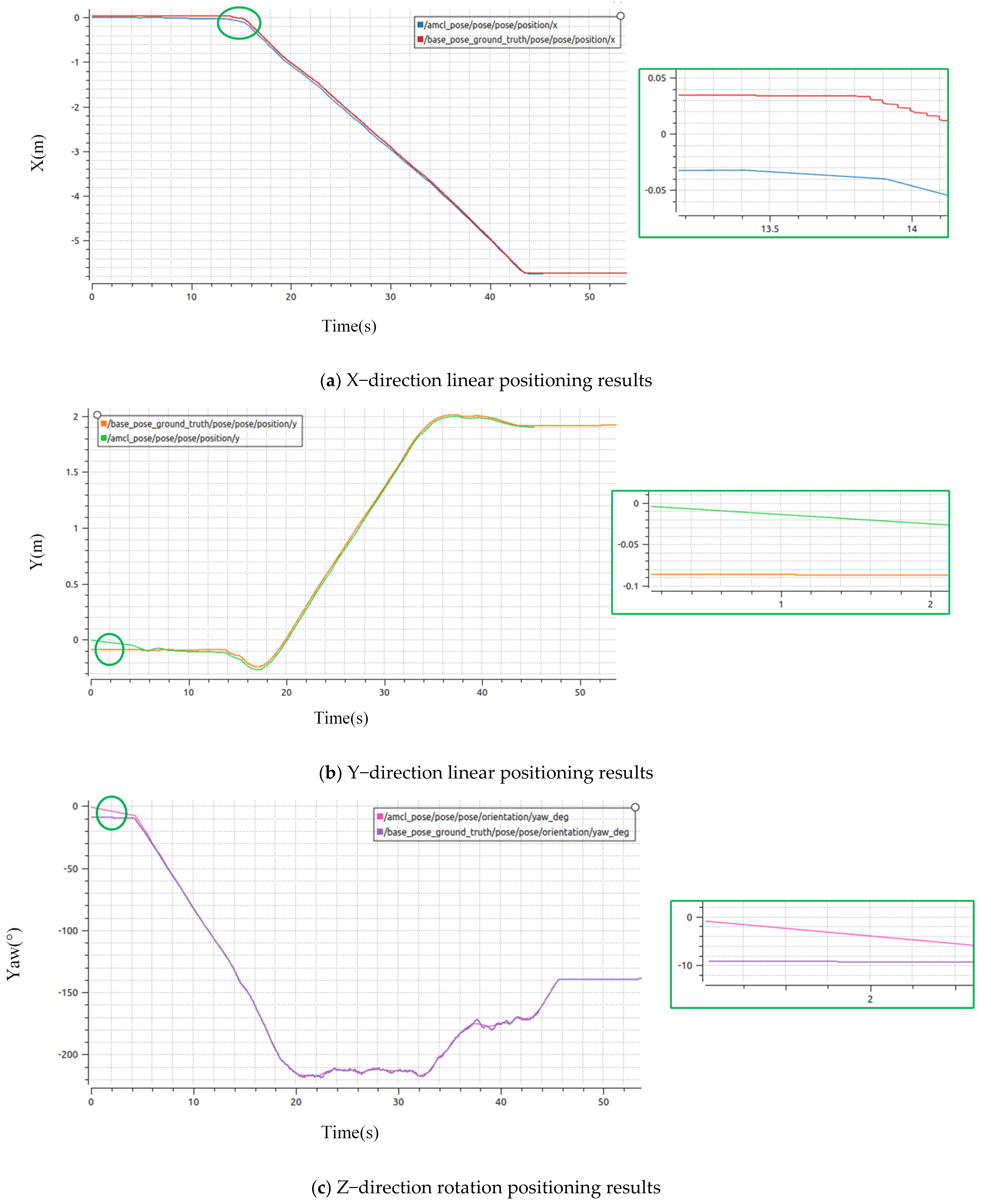
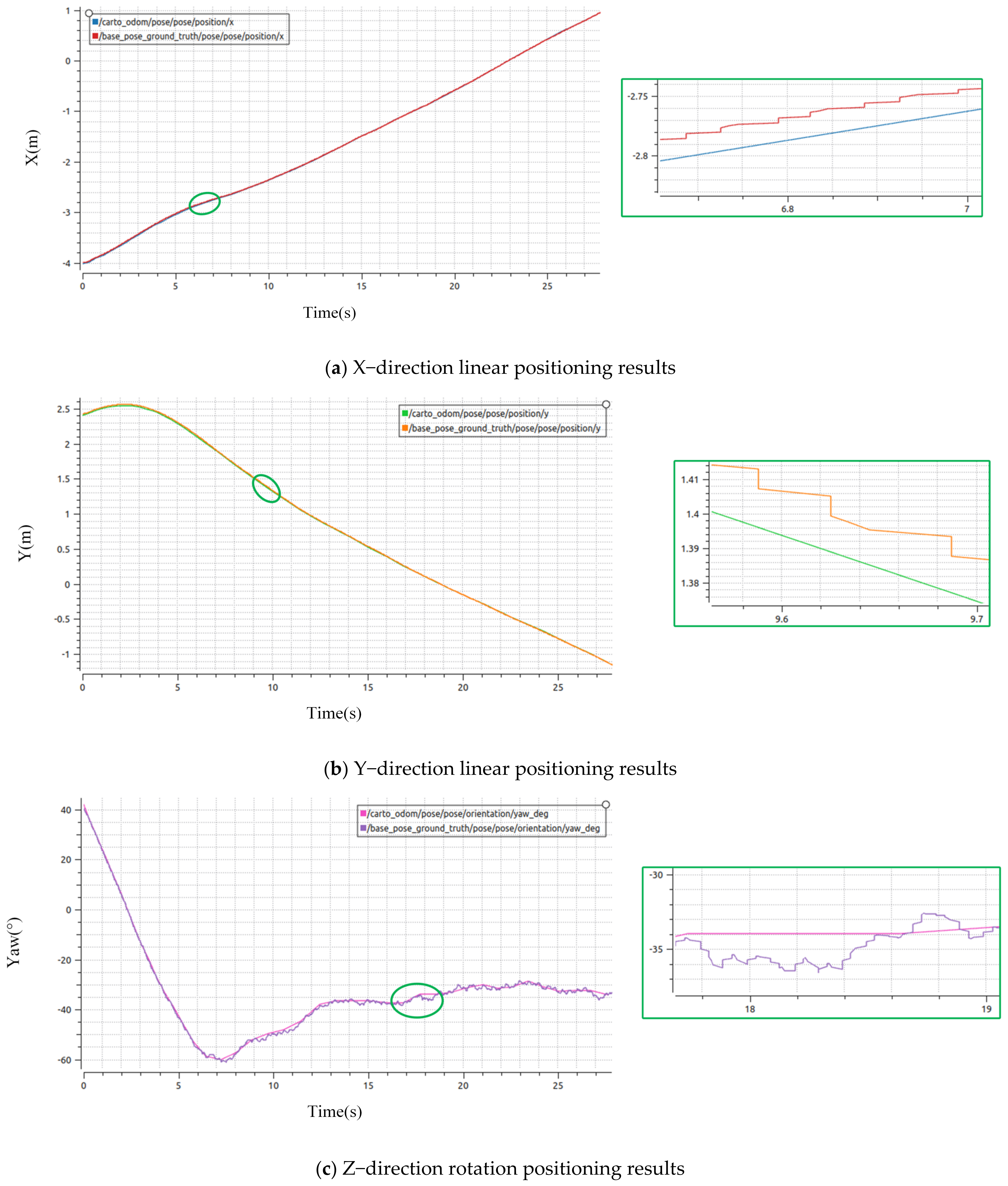
4.1.3. Analysis of Simulation Positioning Results

We conducted three sets of independent simulation comparison experiments on the AMCL algorithm: the improved AMCL algorithm in this paper, the cartographer algorithm method (3D localization, the maximum number of saved subgraphs is 3, and the effective number of frames per subgraph is 20) and the hdl_localization algorithm (a NDT-based localization algorithm).

During the simulation experiments, we randomly give the target position to be reached by the robot motion, and after the robot reaches the target position, the localization information of the algorithm during this motion is recorded and compared with the real values in the simulation environment. The localization results of AMCL are shown in Figure 6, Figure 7 and Figure 8, the localization results of the modified AMCL algorithm are shown in Figure 9, Figure 10 and Figure 11, the localization results of the cartographer are shown in Figure 12, Figure 13 and Figure 14 and the localization results of hdl_localization are shown in Figure 15, Figure 16 and Figure 17.

From Figure 6, Figure 7 and Figure 8, it can be seen that the linear positioning and angular positioning results of the original AMCL algorithm have large errors with the actual values, and especially, the curve fitting of the yaw angle is poor. There are many fluctuations, and the fluctuation magnitude is large.

From Figure 9, Figure 10 and Figure 11, it can be seen that the linear positioning and angular positioning results of the original AMCL algorithm improved in this paper have less error with the actual values, and the curve fitting of the yaw angle is better with less fluctuation and smaller amplitude.

From Figure 12, Figure 13 and Figure 14, it can be seen that the cartographer algorithm linear positioning and angular positioning results are stable and fit well with the real values with small errors, especially since the yaw angle positioning is smooth with very small fluctuations.

From Figure 15, Figure 16 and Figure 17, it can be seen that the localization results of hdl_localization are unstable. The method is based on the UKF framework, which fuses IMU data and laser odometer data obtained by NDT matching to achieve localization, and thus is susceptible to the effects of noise and robot speed, resulting in fluctuations and discontinuities in the localization results.

Since localization results of the hdl_localization algorithm are easily affected by noise, which is not conducive to data analysis, we count the maximum localization errors of the other three algorithms in the simulation experiments and include them in

Table 1. Maximum positioning error in the simulation experiment of three algorithms.

Methods	Experiments	Maximum Error in X Direction	Maximum Error in Y Direction	Maximum Error in Yaw Angle
	1	6 cm	6 cm	4 degs
AMCL	2	7 cm	8 cm	8 degs
	3	4 cm	2 cm	6 degs
	1	2 cm	0.5 cm	2.5 degs
Ours	2	2 cm	2.5 cm	3.5 degs
	3	1.5 cm	2 cm	3.5 degs
	1	5 cm	4 cm	3 degs
Cartographer	2	2 cm	3 cm	3 degs
	3	2 cm	1.6 cm	2.5 degs

for data analysis.

Compared with the original AMCL algorithm, the maximum positioning error of the improved AMCL algorithm in this paper is smaller, and the accuracy of both linear and angular positioning is significantly improved. Meanwhile, among these three algorithms, the improved AMCL algorithm in this paper has a good advantage in linear positioning accuracy. The maximum positioning error of the cartographer algorithm is more stable, the overall positioning accuracy of the algorithm is better than that of the AMCL algorithm and the angular positioning accuracy is slightly better than that of the improved AMCL algorithm in this paper.

4.2. Practical Experiments

4.2.1. Practical Environment

In addition to the above simulation tests, we conducted actual localization experiments in a larger-scale scenario in combination with a mobile robot platform, as shown in Figure 18a. The external measurement system is shown in Figure 18b, which includes a Leica Geosystems absolute tracker (AT960) that can achieve a position accuracy of 0.01 mm and angular accuracy of 0.01 degrees.

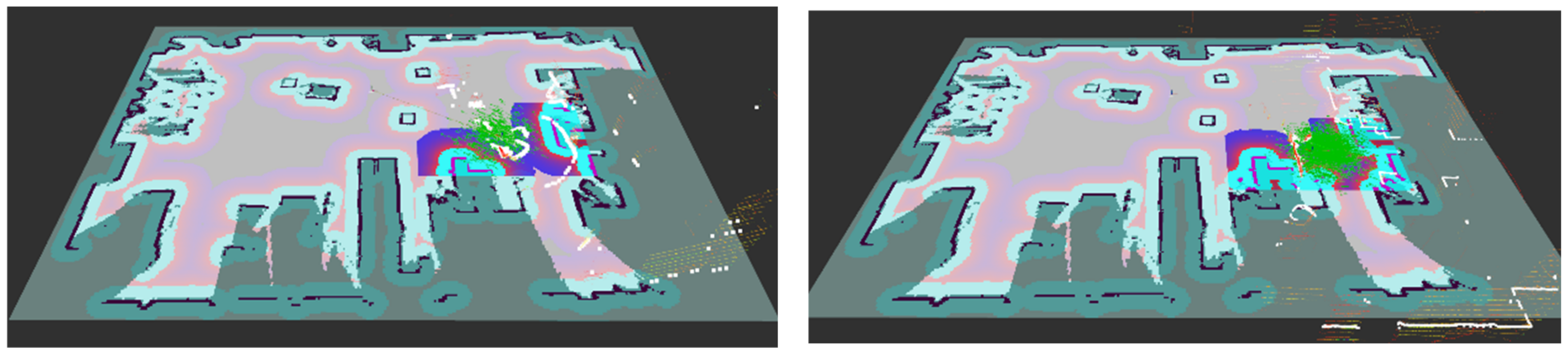
4.2.2. Point Cloud Matching Correction for AMCL Positioning

As in Section 4.1.2, we compare the results before and after the correction of the AMCL positional attitude by the three-dimensional laser odometer in this section. The comparison results are shown in Figure 19. As can be seen in Figure 19, the point cloud correction results in the actual experiment are consistent with the simulation.

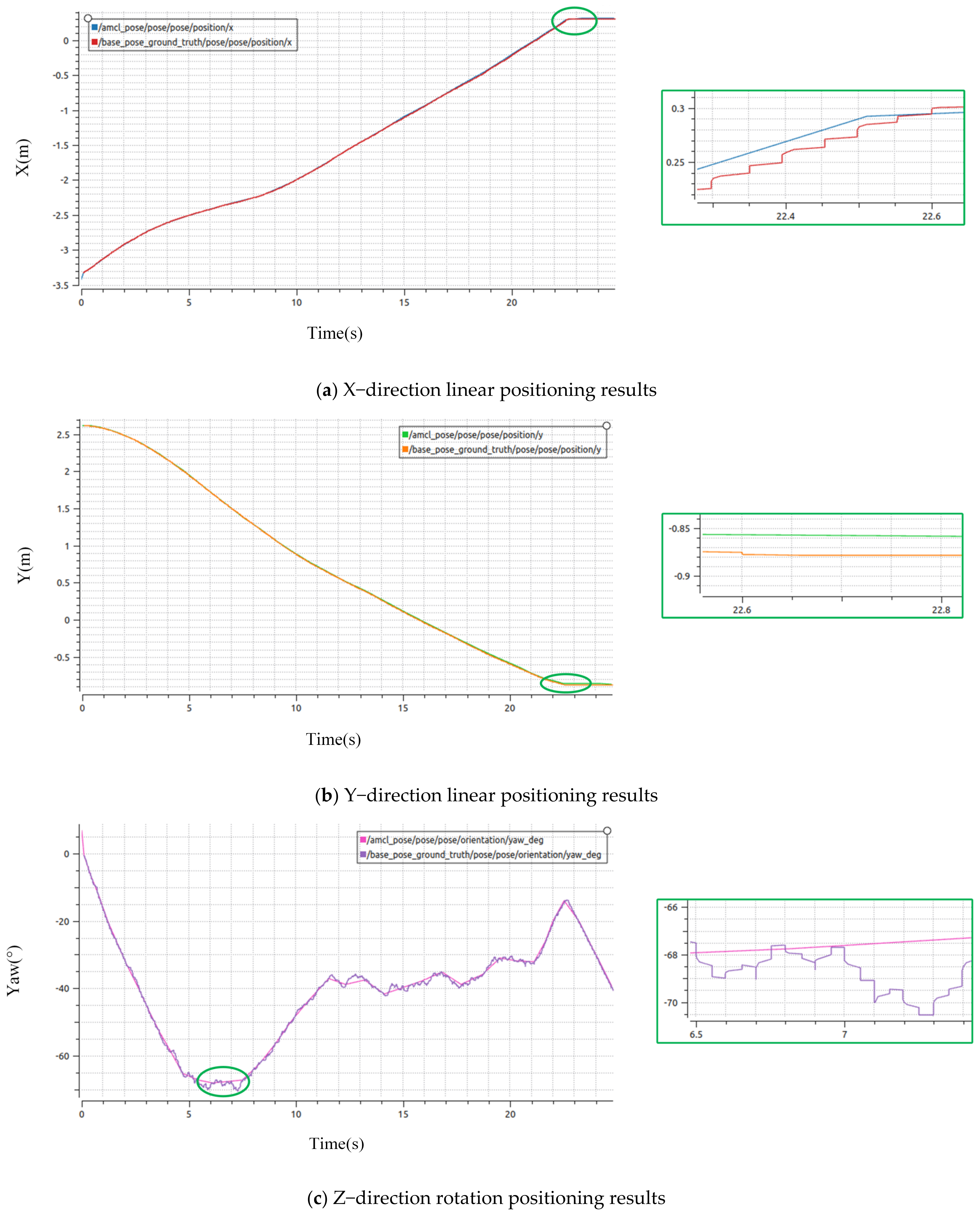
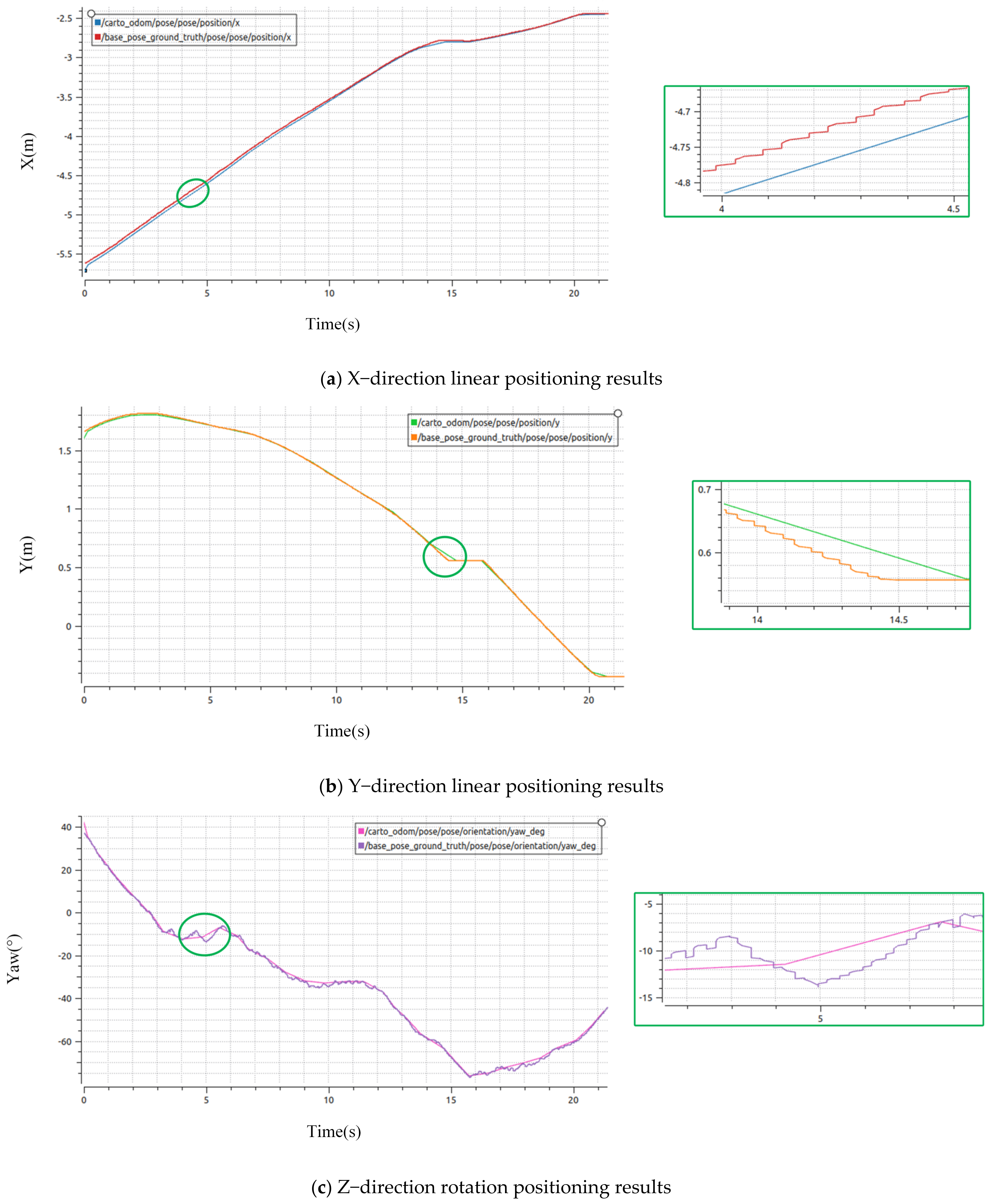
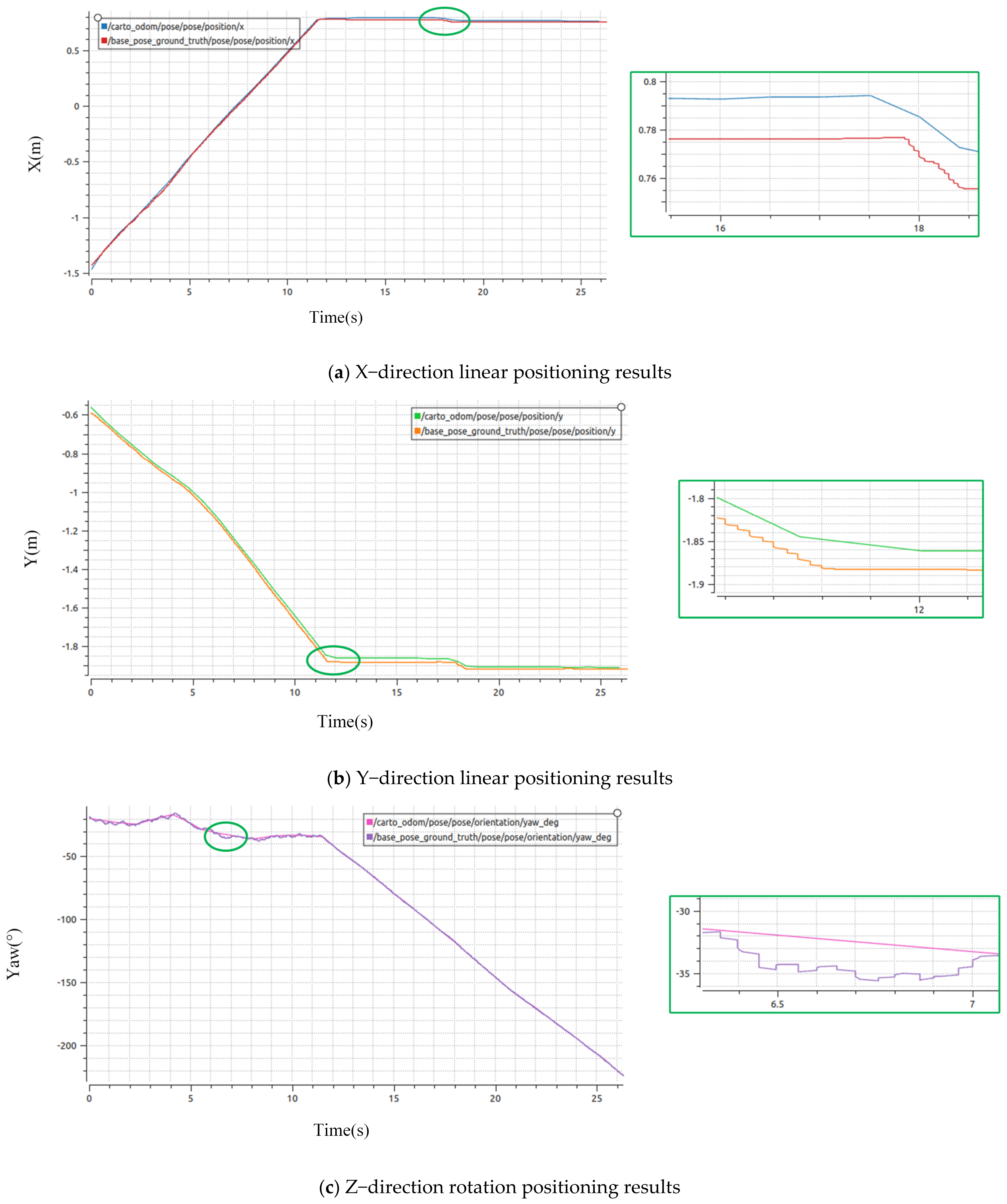
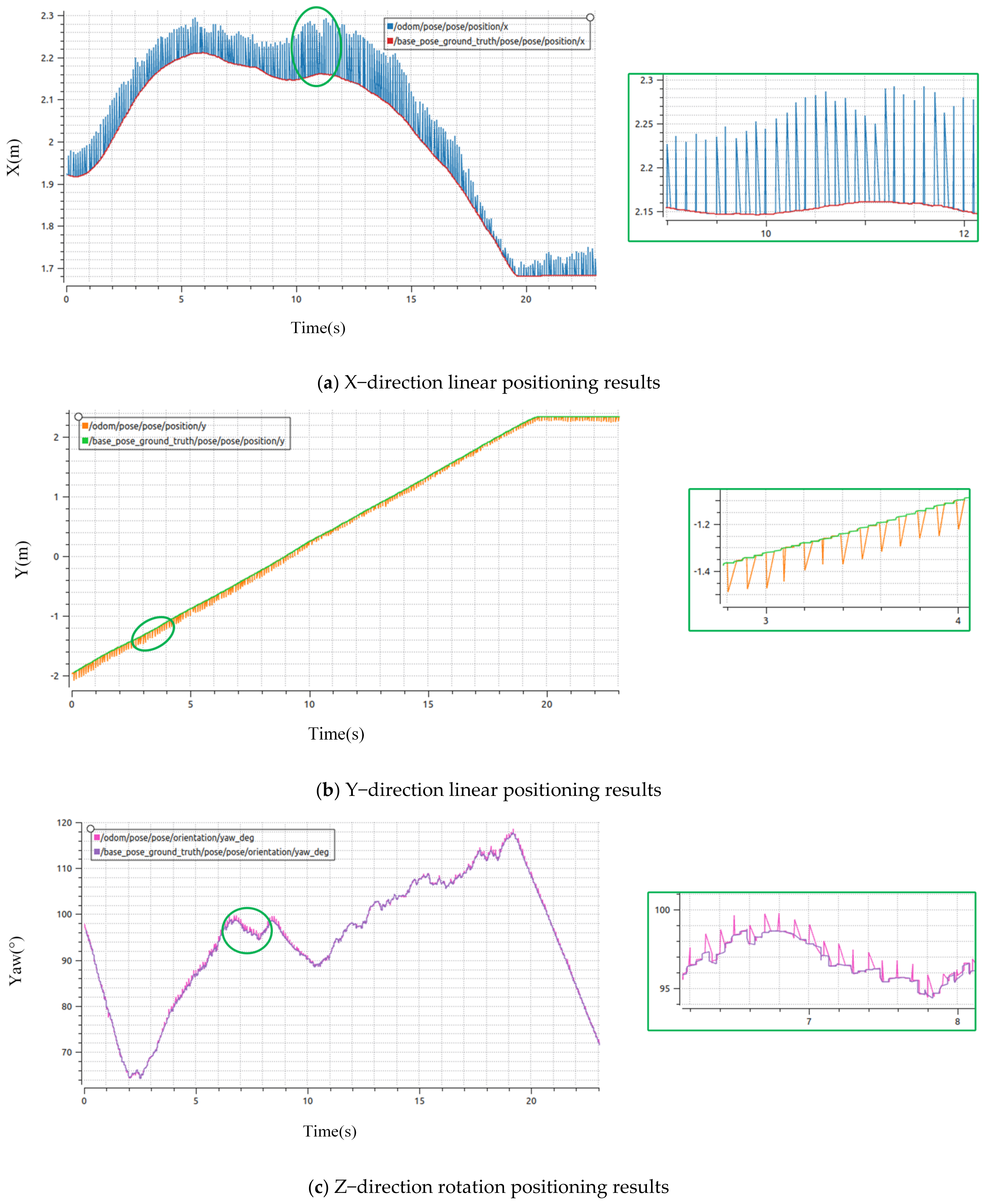
4.2.3. Analysis of Practical Positioning Results

In order to compare the accurate differences between the above four algorithms, we counted the positioning accuracy of the four algorithms in turn after the experimental platform was turned on. We randomly gave the robot 30 target positions in the experimental site, and when the robot reached the target position, we recorded the positioning information printed by the terminal, including linear direction (X-direction) position information and angular information (yaw angle), and compared with the results of the total station to obtain the positioning error.

The hdl_localization algorithm is less stable due to drift and failure during multiple successive localizations, so we collected data and mathematical statistics on the localization errors of the other three algorithms. The actual localization results of the three algorithms are shown in Figure 20, and the mathematical and statistical results of the three algorithms are shown in

Table 2. Three algorithms positioning error analysis.

Method	Position Mean (m)	Position Std (m)	Yaw Mean (°)	Yaw Std (°)
AMCL	0.094	0.0329	9.183	2.383
Ours	0.061	0.0236	6.097	1.171
Cartographer	0.079	0.0260	5.540	1.135

.

From Figure 20, it can be seen that among the three algorithms, the improved AMCL algorithm in this paper has the best linear directional localization accuracy; the cartographer algorithm has the second best, and the original AMCL algorithm has the lowest linear localization accuracy. The cartographer algorithm has the best yaw angle localization accuracy, the improved AMCL algorithm in this paper is the second best and the original AMCL algorithm is the worst.

As can be seen from Table 2, the improved AMCL algorithm in this paper has the highest linear localization accuracy compared with the original AMCL algorithm and the cartographer algorithm. Compared with the original AMCL algorithm, the improved AMCL algorithm in this paper has reduced the average positioning error in linear direction by 0.033 m, which means that the linear direction positioning accuracy is improved by 35%, and the average positioning error in yaw angle is reduced by 3.086°, which means that the yaw angle positioning accuracy is improved by 34%. Although the positioning algorithm proposed in this paper achieves good results, the positioning accuracy of the yaw angle still needs to continue to be improved compared with the cartographer algorithm. Compared with the cartographer algorithm, the AMCL algorithm improved in this paper reduces the average positioning error by 0.018 m in the straight line direction, which means the linear positioning accuracy is improved by 23%, and the average positioning error of the yaw angle is only about 0.557°.

By comparing the standard deviations, it can be seen that compared with the original AMCL algorithm, the improved AMCL algorithm in this paper has smaller standard deviations for both linear orientation positioning and yaw angle positioning values, indicating that the improved algorithm has better positioning stability. However, the improved AMCL algorithm in this paper is deficient in the positioning accuracy and stability of the yaw angle compared with the cartographer algorithm.

5. Discussions

5.1. Discussion of Simulation Results

Combining the experimental simulation results of the four algorithms and the analysis of positioning accuracy and stability, the improved AMCL algorithm in this article has the best positioning effect, significantly improves the positioning accuracy of the original AMCL algorithm and ensures the stability of the algorithm. The cartographer algorithm has stable positioning results in the positioning process and has obvious advantages in yaw angle positioning accuracy. The original AMCL algorithm has large errors in both linear localization and angular localization, but the algorithm itself has good stability. The hdl_localization algorithm is more affected by noise, and the localization results are not stable enough.

5.2. Discussion of Actual Results

We conducted comparison experiments on the original AMCL algorithm, the improved AMCL algorithm in this paper and the cartographer algorithm and analyzed them together with the actual localization results. In the process of straight-line positioning, the improved AMCL algorithm has the best accuracy, the cartographer algorithm has the second-best accuracy and the AMCL algorithm has the worst accuracy. In the process of angular positioning, the cartographer positioning accuracy is the best, the improved AMCL algorithm is the second best, there is a small gap with the cartographer algorithm and the original AMCL algorithm is the worst.

6. Conclusions

We improve the AMCL algorithm and propose a localization method applicable to 3D LiDAR. The method significantly improves the localization accuracy of AMCL algorithm by technical means of multi-sensing information fusion and 3D point cloud-assisted localization. However, the positioning accuracy and stability of the yaw angle are deficient compared with the cartographer algorithm. The positioning method proposed in this paper introduces a 3D point cloud alignment correction, which increases the computation time of the algorithm. Subsequent optimization of the point cloud alignment algorithm is needed in order to shorten the positioning time of the method and improve the positioning accuracy.

References

1. Jie, L.; Jin, Z.; Wang, J.; Zhang, L.; Tan, X. A SLAM System with Direct Velocity Estimation for Mechanical and Solid-State LiDARs. Remote Sens. 2022, 14, 1741. [Google Scholar] [CrossRef]
2. Pfaff, P.; Burgard, W.; Fox, D. Robust monte-carlo localization using adaptive likelihood models. In European Robotics Symposium 2006; Springer: Berlin/Heidelberg, Germany, 2006; pp. 181–194. [Google Scholar]
3. Fox, D.; Burgard, W.; Dellaert, F.; Thrun, S. Monte carlo localization: Efficient position estimation for mobile robots. AAAI IAAI 1999, 2, 343–349. [Google Scholar]
4. Yang, J.; Wang, C.; Luo, W.; Zhang, Y.; Chang, B.; Wu, M. Research on Point Cloud Registering Method of Tunneling Roadway Based on 3D NDT-ICP Algorithm. Sensors 2021, 21, 4448. [Google Scholar] [CrossRef] [PubMed]
5. Chiang, K.W.; Tsai, G.J.; Li, Y.H.; Li, Y.; El-Sheimy, N. Navigation engine design for automated driving using INS/GNSS/3D LiDAR-SLAM and integrity assessment. Remote Sens. 2020, 12, 1564. [Google Scholar] [CrossRef]
6. Sefati, M.; Daum, M.; Sondermann, B.; Kreisköther, K.D.; Kampker, A. Improving vehicle localization using semantic and pole-like landmarks. In Proceedings of the 2017 IEEE Intelligent Vehicles Symposium (IV), Los Angeles, CA, USA, 11–14 June 2017; pp. 13–19. [Google Scholar]
7. Tee, Y.K.; Han, Y.C. Lidar-Based 2D SLAM for Mobile Robot in an Indoor Environment: A Review. In Proceedings of the 2021 International Conference on Green Energy, Computing and Sustainable Technology (GECOST), Miri, Malaysia, 7–9 July 2021; pp. 1–7. [Google Scholar]
8. Zhang, T.; Zhang, X. A mask attention interaction and scale enhancement network for SAR ship instance segmentation. IEEE Geosci. Remote Sens. Lett. 2022, 19, 1–5. [Google Scholar] [CrossRef]
9. Zhang, T.; Zhang, X. HTC+ for SAR Ship Instance Segmentation. Remote Sens. 2022, 14, 2395. [Google Scholar] [CrossRef]
10. Zhang, T.; Zhang, X. A polarization fusion network with geometric feature embedding for SAR ship classification. Pattern Recognit. 2022, 123, 108365. [Google Scholar] [CrossRef]
11. Jiang, Z.; Liu, B.; Zuo, L.; Zhang, J. High Precise Localization of Mobile Robot by Three Times Pose Correction. In Proceedings of the 2018 2nd International Conference on Robotics and Automation Sciences (ICRAS), Wuhan, China, 23–25 June 2018; pp. 1–5. [Google Scholar]
12. Zhang, T.; Zhang, X.; Liu, C.; Shi, J.; Wei, S.; Ahmad, I.; Zhan, X.; Zhou, Y.; Pan, D.C.; Su, H. Balance learning for ship detection from synthetic aperture radar remote sensing imagery. ISPRS J. Photogramm. Remote Sens. 2021, 182, 190–207. [Google Scholar] [CrossRef]
13. Zhang, T.; Zhang, X. High-speed ship detection in SAR images based on a grid convolutional neural network. Remote Sens. 2019, 11, 1206. [Google Scholar] [CrossRef] [Green Version]
14. Zhang, T.; Zhang, X.; Shi, J.; Wei, S. Depthwise separable convolution neural network for high-speed SAR ship detection. Remote Sens. 2019, 11, 2483. [Google Scholar] [CrossRef] [Green Version]
15. De Miguel, M.Á.; García, F.; Armingol, J.M. Improved LiDAR probabilistic localization for autonomous vehicles using GNSS. Sensors 2020, 20, 3145. [Google Scholar] [CrossRef]
16. Liu, Y.; Zhao, C.; Wei, Y. A Robust Localization System Fusion Vision-CNN Relocalization and Progressive Scan Matching for Indoor Mobile Robots. Appl. Sci. 2022, 12, 3007. [Google Scholar] [CrossRef]
17. Ge, G.; Zhang, Y.; Wang, W.; Jiang, Q.; Hu, L.; Wang, Y. Text-MCL: Autonomous mobile robot localization in similar environment using text-level semantic information. Machines 2022, 10, 169. [Google Scholar] [CrossRef]
18. Obregón, D.; Arnau, R.; Campo-Cossío, M.; Nicolás, A.; Pattinson, M.; Tiwari, S.; Ansuategui, A.; Tubío, C.; Reyes, J. Adaptive Localization Configuration for Autonomous Scouting Robot in a Harsh Environment. In Proceedings of the 2020 European Navigation Conference (ENC), Dresden, Germany, 23–24 November 2020; pp. 1–8. [Google Scholar]
19. Fikri, A.A.; Anifah, L. Mapping and Positioning System on Omnidirectional Robot Using Simultaneous Localization and Mapping (Slam) Method Based on Lidar. J. Teknol. 2021, 83, 41–52. [Google Scholar] [CrossRef]
20. Portugal, D.; Araújo, A.; Couceiro, M.S. A reliable localization architecture for mobile surveillance robots. In Proceedings of the 2020 IEEE International Symposium on Safety, Security, and Rescue Robotics (SSRR), Abu Dhabi, United Arab Emirates, 4–6 November 2020; pp. 374–379. [Google Scholar]
21. Shen, K.; Wang, M.; Fu, M.; Yang, Y.; Yin, Z. Observability analysis and adaptive information fusion for integrated navigation of unmanned ground vehicles. IEEE Trans. Ind. Electron. 2019, 67, 7659–7668. [Google Scholar] [CrossRef]
22. Xu, X.; Zhang, L.; Yang, J.; Cao, C.; Wang, W.; Ran, Y.; Tan, Z.; Luo, M. A Review of Multi-Sensor Fusion SLAM Systems Based on 3D LIDAR. Remote Sens. 2022, 14, 2835. [Google Scholar] [CrossRef]
23. Dempster A, P. New methods for reasoning towards posterior distributions based on sample data. Ann. Math. Stat. 1966, 37, 355–374. [Google Scholar] [CrossRef]
24. Germain, M.; Voorons, M.; Boucher, J.M.; Benie, G.B. Fuzzy statistical classification method for multiband image fusion. In Proceedings of the Fifth International Conference on Information Fusion. FUSION 2002. (IEEE Cat. No. 02EX5997), Annapolis, MD, USA, 8–11 July 2002; pp. 178–184. [Google Scholar]
25. Chin, L. Application of neural networks in target tracking data fusion. IEEE Trans. Aerosp. Electron. Syst. 1994, 30, 281–287. [Google Scholar] [CrossRef]
26. Thrun, S.; Burgard, W.; Fox, D. Probabilistic Robotics; China Machine Press: Beijing, China, 1999; pp. 1–11. [Google Scholar]
27. Xiang, X.; Li, K.; Huang, B.; Cao, Y. A Multi-Sensor Data-Fusion Method Based on Cloud Model and Improved Evidence Theory. Sensors 2022, 22, 5902. [Google Scholar] [CrossRef]
28. Hartigan, J.A.; Wong, M.A. Algorithm AS 136: A k-means clustering algorithm. J. R. Stat. Soc. Ser. C Appl. Stat. 1979, 28, 100–108. [Google Scholar] [CrossRef]
29. Chen, F.C.; Jahanshahi, M.R. NB-CNN: Deep learning-based crack detection using convolutional neural network and Naïve Bayes data fusion. IEEE Trans. Ind. Electron. 2017, 65, 4392–4400. [Google Scholar] [CrossRef]
30. Xu, W.; Zhang, F. Fast-lio: A fast, robust lidar-inertial odometry package by tightly-coupled iterated kalman filter. IEEE Robot. Autom. Lett. 2021, 6, 3317–3324. [Google Scholar] [CrossRef]
31. Zhao, S.; Gu, J.; Ou, Y.; Zhang, W.; Pu, J.; Peng, H. IRobot self-localization using EKF. In Proceedings of the 2016 IEEE International Conference on Information and Automation (ICIA), Ningbo, China, 31 July–4 August 2016; pp. 801–806. [Google Scholar]
32. Aybakan, T.; Kerestecioğlu, F. Indoor positioning using federated Kalman filter. In Proceedings of the 2018 3rd International Conference on Computer Science and Engineering (UBMK), Sarajevo, Bosnia and Hercegovina, 20–23 September 2018; pp. 483–488. [Google Scholar]
33. Feng, J.; Wang, Z.; Zeng, M. Distributed weighted robust Kalman filter fusion for uncertain systems with autocorrelated and cross-correlated noises. Inf. Fusion 2013, 14, 78–86. [Google Scholar] [CrossRef]
34. Julier, S.J.; LaViola, J.J. On Kalman filtering with nonlinear equality constraints. IEEE Trans. Signal Process. 2007, 55, 2774–2784. [Google Scholar] [CrossRef] [Green Version]
35. Xu, X.; Pang, F.; Ran, Y.; Bai, Y.; Zhang, L.; Tan, Z.; Wei, C.; Luo, M. An indoor mobile robot positioning algorithm based on adaptive federated Kalman Filter. IEEE Sens. J. 2021, 21, 23098–23107. [Google Scholar] [CrossRef]
36. Moravec, H.; Elfes, A. High resolution maps from wide angle sonar. In Proceedings of the 1985 IEEE International Conference on Robotics and Automation, St. Louis, MI, USA, 25–28 March 1985; pp. 116–121. [Google Scholar]
37. Wang, J.; Ni, D.; Li, K. RFID-based vehicle positioning and its applications in connected vehicles. Sensors 2014, 14, 4225–4238. [Google Scholar] [CrossRef]
38. Moore, T.; Stouch, D. A generalized extended kalman filter implementation for the robot operating system. In Intelligent Autonomous Systems 13; Springer: Cham, Switzerland, 2016; pp. 335–348. [Google Scholar]
39. Besl, P.J.; McKay, N.D. Method for registration of 3-D shapes. In Sensor Fusion IV: Control Paradigms and Data Structures; SPIE: Bellingham, WA, USA, 1992; pp. 586–606. [Google Scholar]
40. Biber, P.; Straßer, W. The normal distributions transform: A new approach to laser scan matching. In Proceedings of the 2003 IEEE/RSJ International Conference on Intelligent Robots and Systems (IROS 2003), (Cat. No. 03CH37453), Las Vegas, NV, USA, 27–31 October 2003; pp. 2743–2748. [Google Scholar]
41. Censi, A. An ICP variant using a point-to-line metric. In Proceedings of the 2008 IEEE International Conference on Robotics and Automation, Pasadena, CA, USA, 19–23 May 2008; pp. 19–25. [Google Scholar]
42. Segal, A.; Haehnel, D.; Thrun, S. Generalized-icp. In Robotics: Science and Systems; MIT Press: Cambridge, MA, USA, 2009; p. 435. Available online: https://www.robots.ox.ac.uk/~avsegal/resources/papers/Generalized_ICP.pdf (accessed on 12 August 2022).
43. Serafin, J.; Grisetti, G. NICP: Dense normal based point cloud registration. In Proceedings of the 2015 IEEE/RSJ International Conference on Intelligent Robots and Systems (IROS), Hamburg, Germany, 28 September–3 October 2015; pp. 742–749. [Google Scholar]
44. Nüchter, A. Parallelization of Scan Matching for Robotic 3D Mapping; EMCR: Dourdan, French, 2007; Available online: https://robotik.informatik.uni-wuerzburg.de/telematics/download/ecmr2007.pdf (accessed on 12 August 2022).
45. Qiu, D.; May, S.; Nüchter, A. GPU-accelerated nearest neighbor search for 3D registration. In Proceedings of the International Conference on Computer Vision Systems, Liège, Belgium, 13–15 October 2009; Springer: Berlin/Heidelberg, Germany, 2009; pp. 194–203. [Google Scholar]
Figure 1. Framework of improved AMCL localization algorithm based on multi-sensing.
Remotesensing 14 06133 g001
Figure 2. AMCL algorithm flow based on EKF fusion improvement.
Remotesensing 14 06133 g002
Figure 3. Principle of PL-ICP algorithm.
Remotesensing 14 06133 g003
Figure 4. Simulation experiment environment. (a) is the virtual simulation scene, and (b) is the related model of the mobile robot in Gazebo. In (b), the yellow module is the mobile robot chassis, the blue module is the Velodyne 16-line LiDAR, and the red module is the IMU inertial measurement unit.
Remotesensing 14 06133 g004
Figure 5. Point cloud correction before and after navigation map. The left figure shows before correction, and the right figure shows after correction, the white color shows the 2D laser point cloud data obtained after the conversion of 3D laser point cloud data, the green color shows the AMCL algorithm particle swarm, and the light purple part shows the cost map after the expansion.
Remotesensing 14 06133 g005
Figure 6. Results of the first group of AMCL simulation positioning experiments.
Remotesensing 14 06133 g006
Figure 7. Results of the second group of AMCL simulation positioning experiments.
Remotesensing 14 06133 g007
Figure 8. Results of the third group of AMCL simulation positioning experiments.
Remotesensing 14 06133 g008
Figure 9. Results of the first group of improved AMCL simulation positioning experiments.
Remotesensing 14 06133 g009
Figure 10. Results of the second group of improved AMCL simulation positioning experiments.
Remotesensing 14 06133 g010
Figure 11. Results of the third group of improved AMCL simulation positioning experiments.
Remotesensing 14 06133 g011
Figure 12. Results of the first group of cartographer simulation positioning experiments.
Remotesensing 14 06133 g012
Figure 13. Results of the second group of cartographer simulation positioning experiments.
Remotesensing 14 06133 g013
Figure 14. Results of the third group of cartographer simulation positioning experiments.
Remotesensing 14 06133 g014
Figure 15. Results of the first group of hdl_localization simulation positioning experiments.
Remotesensing 14 06133 g015
Figure 16. Results of the second group of hdl_localization simulation positioning experiments.
Remotesensing 14 06133 g016
Figure 17. Results of the third group of hdl_localization simulation positioning experiments.
Remotesensing 14 06133 g017
Figure 18. Experimental equipment. (a) shows the mobile robot platform and (b) shows the Leica Geosystems absolute tracker (AT960).
Remotesensing 14 06133 g018
Figure 19. Point cloud correction before and after navigation map. The left figure shows before correction and the right figure shows after correction, the color shows the initial 3D laser point cloud data and the white color shows the 2D laser point cloud data obtained after conversion.
Remotesensing 14 06133 g019
Figure 20. Actual positioning error of mobile robot. The left figure shows the position error of the mobile robot platform and the right figure shows the angle error of the mobile robot platform.
Remotesensing 14 06133 g020