Article

Predicting Leaf Phenology in Forest Tree Species Using UAVs and Satellite Images: A Case Study for European Beech (Fagus sylvatica L.)

by
Mihnea Ioan Cezar Ciocîrlan
1,2,
Alexandru Lucian Curtu
1 and
Gheorghe Raul Radu
2,*
1
Faculty of Silviculture and Forest Engineering, “Transilvania” University of Braşov, 500123 Braşov, Romania
2
Department of Forest Management, “Marin Drăcea” National Institute for Research and Development in Forestry, 077190 Voluntari, Romania
*
Author to whom correspondence should be addressed.
Remote Sens. 2022, 14(24), 6198; https://doi.org/10.3390/rs14246198
Submission received: 30 October 2022 / Revised: 30 November 2022 / Accepted: 5 December 2022 / Published: 7 December 2022
(This article belongs to the Section Forest Remote Sensing)

Abstract

:
Understanding forest tree phenology is essential for assessing forest ecosystem responses to environmental changes. Observations of phenology using remote sensing devices, such as satellite imagery and Unmanned Aerial Vehicles (UAVs), along with machine learning, are promising techniques. They offer fast, accurate, and unbiased results linked to ground data to enable us to understand ecosystem processes. Here, we focused on European beech, one of Europe’s most common forest tree species, along an altitudinal transect in the Carpathian Mountains. We performed ground observations of leaf phenology and collected aerial images using UAVs and satellite-based biophysical vegetation parameters. We studied the time series correlations between ground data and remote sensing observations (GLI r = 0.86 and FCover r = 0.91) and identified the most suitable vegetation indices (VIs). We trained linear and non-linear (random forest) models to predict the leaf phenology as a percentage of leaf cover on test datasets; the models had reasonable accuracy, RMSE percentages of 8% for individual trees, using UAV, and 12% as an average site value, using the Copernicus biophysical parameters. Our results suggest that the UAVs and satellite images can provide reliable data regarding leaf phenology in the European beech.

1. Introduction

Leaf phenology is a phenomenon that arises from biological processes in plant leaves, which also control the carbon and water cycles [1]. It is the study of monitoring leaf expansion, coloration, and leaf drop during the plant growing season [2]. By monitoring plants’ phenology, one can quantify changes in ecosystem processes such as photosynthesis and transpiration [3] and evaluate the impacts of climate change on ecosystems [4]. Seasonal changes can be studied from a global scale to individual trees and describe the intra- and inter-species tree strategies of adaptability [5]. Currently, there is a trend of increasing annual temperatures, which becomes more noticeable during the tree species’ growing season [6]. The effects of this trend on the Earth’s surface can be identified in the prevalence of processes such as desertification and melting glaciers; melting glaciers cause rising sea levels, indirectly affecting soil erosion [7]. As a result of climate changes, forest tree species are forced to adapt and react through their regulation mechanisms. Therefore, the abilities of forest tree species to respond to the effects of climate change will be increasingly put under pressure and even pushed to their limits of survival. Therefore, it is of growing interest to explain the phenological patterns in the context of these changes [8], especially by reading the spectral variation during the growing season through high-resolution images from both UAVs and satellites [9].
Field observations of tree phenology offer valuable information regarding tree-level monitoring, but they are labor-intensive [10]. Time series observations of spring phenology and senescence may lead to a better understanding of the effect of climate variability or climate change on plant biological events in direct correlation with temperature and precipitation [11], and genetic variability among bio-groups could be determined with a spatial assessment [12]. Often, in multi-layered stands or closed canopies, evaluation from the ground by a single observer can be complex, and errors can occur. Lately, remote sensing technology, such as UAVs, and satellite imagery, have gained attention for their potential use in monitoring phenology and other biological processes [13]. Images collected from satellite sensors have provided essential information regarding the quantification of leaf phenology. However, they are limited by weather conditions (clouds, wind, rain, and fog) and their resolution, providing insufficient data, as seen in some studies regarding individual tree-level analyses [14]. Phenocams have been used successfully in the quantification of forest leaf phenology at individual tree levels, with high frequency, without being obscured by weather conditions [15]. However, they have provided insufficient sample sizes for intra- and interspecific variation analyses, being limited to certain specific trees. Another type of near-surface remote sensing technology that can capture species-specific phenology [16], UAV-mounted sensors, has also been proven effective in providing information for intra- and interspecific variation analyses. Images collected from UAVs provide a clear, unobstructed overview of a canopy and can be used to monitor individual phenological patterns in relatively large areas [4] and for a high number of trees [10], but they also offer a good overview of the tree crown at a branch-level resolution [3,17], which can be linked with ground measurements of trees [3]. UAV devices are becoming more affordable and abundant, thus becoming a viable technology that will probably be complementary to satellite and plane image collection [18]. UAV observations are a robust approach to quantifying the start and the end of the growing season at the individual level [17]. Satellite imagery is considered a large-scale product [18], and monitoring intraspecific tree biological processes such as phenology is challenging. Cloud conditions influence the images, and it can be time-consuming to produce a clear product. However, the Copernicus Global Land Service is a free and open-access data platform that offers access to a series of biophysical products regarding the status and evolution of the land surface at a global scale. Satellites are the only instrument used for extensive and global-scale monitoring. The biophysical parameters of the Copernicus program have a high potential to monitor the changes in the ecosystems, habitats, and land cover. These high spatial resolution products provide means to quantify the phenology and productivity [19] and interannual variability of ecosystems.
The VIs are single values based on various combinations of reflected radiation of two or more wavelengths derived from vegetation’s reflectance properties. Typically, they quantify the red, green, blue, and near-infrared (NIR) band lengths. They are widely used to monitor tree phenology [5,10,18,20] and crop plant development [21,22] by quantifying chlorophyll or leaf nitrogen content [23,24,25]. The image acquisition conditions such as brightness, angle of reflectance, or stability can significantly impact the VIs observed values [21] of the same scene. Although the Normalized Difference Vegetation Index (NDVI) is a widely used VI to monitor the vegetative cover [4,13,16] and is strongly correlated with chlorophyll content [23] by using near-infrared light (NIR), it is limited to multispectral or hyperspectral cameras. Nevertheless, good results in monitoring tree phenology during the growing season were obtained using VIs collected with image sensors based only on red, green, and blue (RGB) colors [4,26].
The European beech (Fagus sylvatica L.) has a large distribution area and high economic value. However, the competitive capacity of the European beech might be reduced due to climate change [27], as it is a tree species that prefers a moderate climate, avoiding extremities in temperature [28]. Thus, to more effectively understand local adaptation, it is necessary to monitor and analyze the phenological expressions of forest tree species with regard to climate factors [29]. The European beech stores high quantities of carbon in its biomass and has good malleability in terms of adaptation to new ecological conditions, a wide range of products of wood use, and resistance to pests and diseases. All of these characteristics provide reasonable justification for the study of this forest tree species [30].
In this paper, we aimed to assess the potential of studying the leaf phenology of the European beech in both individual trees by UAV systems equipped with an RGB camera and as average site percentage of leaf cover through the biophysical parameters collected from the Copernicus data platform. The main objective was to assess leaf phenology (leaf unfolding and senescence) during a growing season across an altitudinal gradient. Specifically, we asked: (1) What are the most useful UAV-based imagery VIs for assessing/ predicting leaf phenology at individual tree levels? (2) what are the most appropriate biophysical parameters derived from the Copernicus satellite for assessing site-level leaf phenology?

2. Materials and Methods
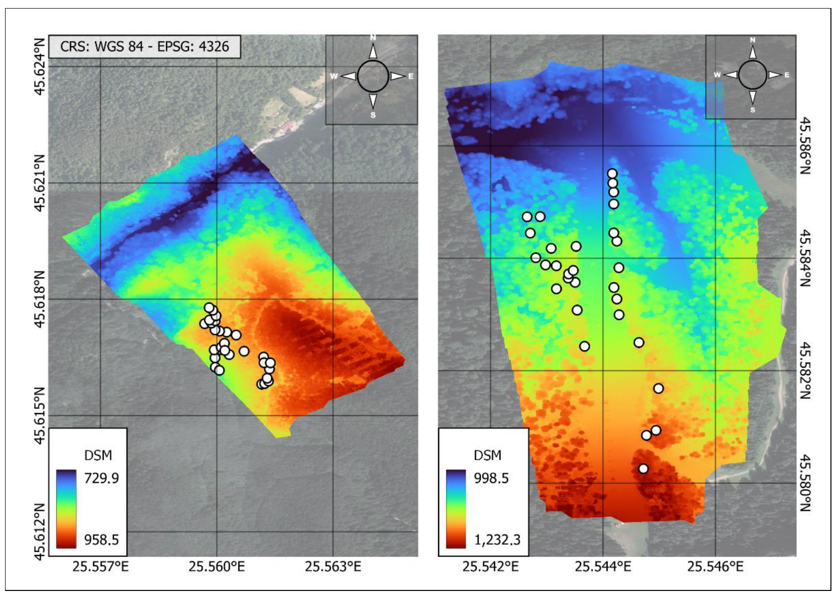
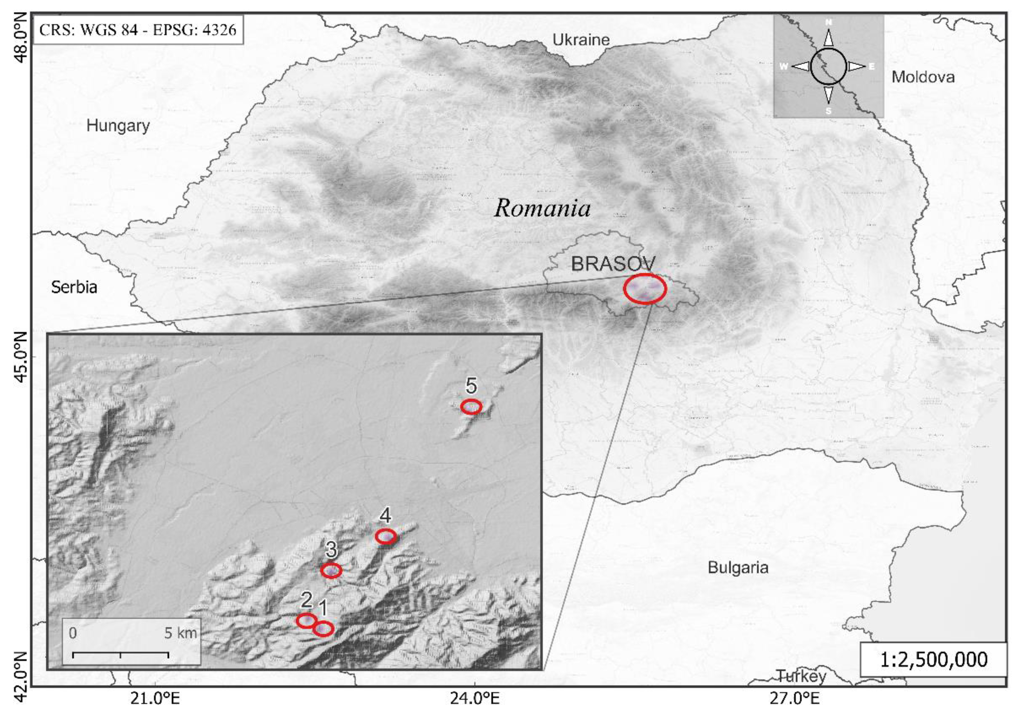
2.1. Study Sites

The study was performed along an altitudinal transect in the South-Eastern Carpathians Mountains (Figure 1). The distribution of beech trees in the studied area covers an altitude ranging from 1450 m in Site 1 to 550 m in Site 5 (Table 1, Figure 1). In each of the five study sites, 30 individual adult beech trees located at a minimum distance of at least 25 m from each other were analyzed. All individuals were selected on north-facing slopes.
The study sites overlapped with the natural beech range in the Brasov area, located on a 20 km transect with a 900 m elevation difference. These were chosen in mixed stands, where the European beech forms mixtures with other deciduous trees, such as hornbeam and sycamore, and conifers, such as the Norway spruce and silver fir. The age of these stands ranges from 80 to 120 years.

2.2. Ground Phenological Observations

The methodology proposed by Vitasse [31] was used during the fieldwork. It is an observation procedure of the phenology that showed promising results [32]. The populations studied were sampled along the altitude gradient following the clinal variation. This sampling was justified by the subsequent possibility of performing analyses on buds, specifically to determine apical bud phenology.
In these five study sites, we monitored the timing of leaf unfolding (LU) and senescence during the 2021 growing season. We visited each population twice a week, from April to June and September to November, to carry out phenological observations. These observations were made with the naked eye or using binoculars, with a magnifying power of 10×. These observations were always carried out by the same observer, approximately 15 m away from the individual.

2.2.1. Leaf Unfolding

The development stages of buds, from dormancy to LU, were correlated with values of the following scale (Table 2):
Furthermore, this quality scale comprising the stages of the phenophase of bud opening and LU for the European beech (Table 2) was converted into a quantitative scale in order to determine the units of exact measurement and to compare them with the results obtained from the processing of images taken from the UAV devices and biophysical parameters from Copernicus.
Subsequently, we visually assessed the proportion of buds in the last stage of development. These stages were assigned to each tree via linear interpolation between two consecutive data field observations. For a bud, we considered the LU stage to have been reached when at least one of its leaves was fully unfolded. For an individual tree, we considered the leaf unfolding date (LUD) to be when at least 50% of the buds had reached this stage. We calculated the LU for each study site population as the average of the estimated LUD for the 30 sampled individuals.

2.2.2. Senescence

In autumn, we assessed the percentage of missing leaves and the percentage of colored leaves from the total remaining ones in the canopy visually, according to the following formula [31]:
%CFL = (%CL × (100 − %FL))/100 + %FL,
where: %CFL is the % of colored or fallen leaves, %CL is the % of colored leaves, %FL is the % of fallen leaves.

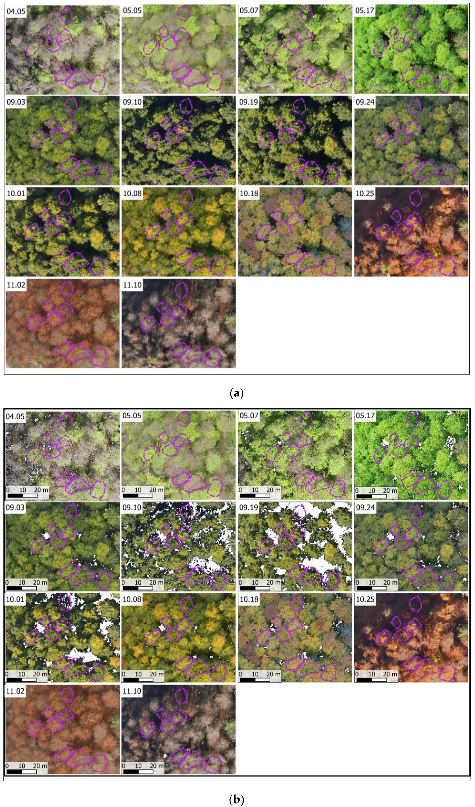
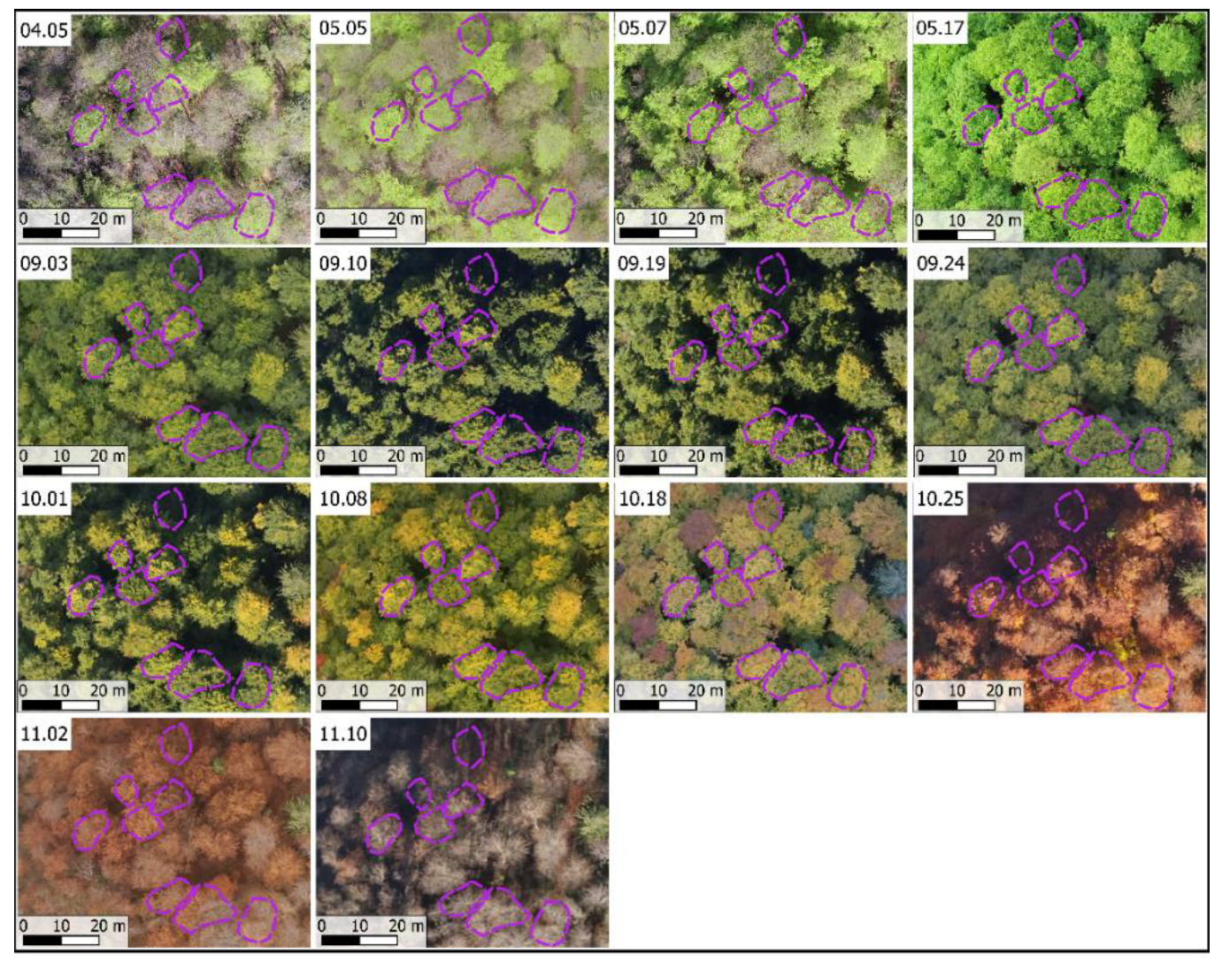
2.3. Time Series Data Collection of Phenological Observations and Image Processing Using UAVs

2.3.1. Image Acquisition

In Site 2 and Site 3 (Table 1), the 60 studied trees and the ground control point’s precise coordinates were collected using Global Navigation Satellite System (GNSS) surveying equipment. Simultaneously with the field observations of trees’ phenological state in two studied sites, aerial images were collected using a UAV.
We used a Phantom 4 Pro v2 model equipped with a Red Green Blue sensor (RGB) of 1-inch CMOS with 20 Megapixel (effective pixels) and lens FOV 84° 8.8 mm/24 mm (35 mm equivalent format) f/2.8 − f/11. The automatic flight missions were created using PIX4Dcapture [33] software to cover the studied trees. Due to the rough terrain in the two sites (Appendix A Figure A1), we used double grid missions to capture pictures at a 70° camera angle and 80%/ 60% overlap for a high-quality result of the Digital Surface Model, which increased the quality of the resulted ortho-photo. The flight missions were performed at an altitude of 150 m (minimal ground sample distance, GSD of 4 cm/px). For each flight, we used the same parameter flight missions. All flights were performed, as much as possible, at midday with constant light conditions, either the clear sky or overcast. The flight speed ranged according to the wind condition and was controlled automatically by the software.
A total of 32 flights (total for both locations) were conducted in the growing season of 2021, which collected images during LU and senescence (Figure 2).

2.3.2. UAV Image Processing

A total of 6080 pictures were collected, averaging 190 pictures per flight. The collected images were processed using Open Drone Map [34], open-source software, resulting in an RGB ortho-rectified image for each flight. For all the ortho-photo processing, we used the same workflow parameters, (1) align photos, choosing high accuracy; (2) build dense point cloud, choosing high quality; (3) build Digital Elevation Model; (4) build ortho-photo, choosing blending mode Mosaic. The ortho-photo products were georeferenced using ground control points and QGis software [35]. For each resulted ortho-photo, shady areas were identified by filtering pixels that matched a threshold of RGB values (which were initially estimated from sample identification) and replaced with null values using the raster package in R (Appendix A Figure A2).
Crown delineation was conducted manually for each of the 60 trees, and using rgdal package, the VIs were calculated, and the mean, median and standard error of pixel values was collected at each flight (Table 3).
The dataset used for phenology prediction consists of a matrix of 60 trees at 16 different timelines in the growing season, 960 observations, and 48 predictors.
Based on the resulting ortho-rectified images after each flight, each tree was evaluated using the same phenological scale in order to be able to make the first comparison between the ground observations and image assessments. The phenology evaluation was made by experts who were not involved in the fieldwork.

2.4. Time Series Data Collection of Phenological Observations and Image Processing Using Copernicus Biophysical Parameters

2.4.1. Data Collection

The Copernicus Global Land Service is a free and open-access data platform that is a part of the European Union’s Earth observation program [44]. It produces a series of bio-geophysical products related to the status and evolution of the land surface at a global scale, which can cover long-term time series.
The remote sensing products in raster format, available from the Copernicus Land Monitoring service portal [44], were collected between April and November 2021 for 19-time dates for each of the five studied locations. The biophysical parameters are provided at a resolution of 300 m, based on Sentinel-3/OLCI data (for the period from 2014-present), at a near real-time (10-daily). To estimate the phenological stage of each studied site, the pixel values of five biophysical parameters were collected: the dry matter productivity, the fraction of absorbed photosynthetically active radiation, the fraction of vegetation cover, the Leaf Area Index, and the Normalized Difference Vegetation Index. The parameters extracted from Copernicus were collected from datasets in a similar period to the ground observations (Table 4).
The FCover is helpful for environmental applications; it corresponds to the fraction of ground covered by green foliage and thus offers a temporal evolution of the land cover changes, while LAI includes all the green vegetative elements that describe woody areas. DMP is developed to estimate vegetation growth from the beginning of the starting season onwards and can detect anomalies in plant development. At the same time, FAPAR can play a role in evaluating carbon balance and monitoring the annual vegetation photosynthetic activity.

2.4.2. Data Processing Analysis

The biophysical parameters data collected during the 2021 growing season consisted of 95 raster datasets from which mean pixel values were collected for each site through the rgdal package of the R software [45].

2.5. Statistical Analysis

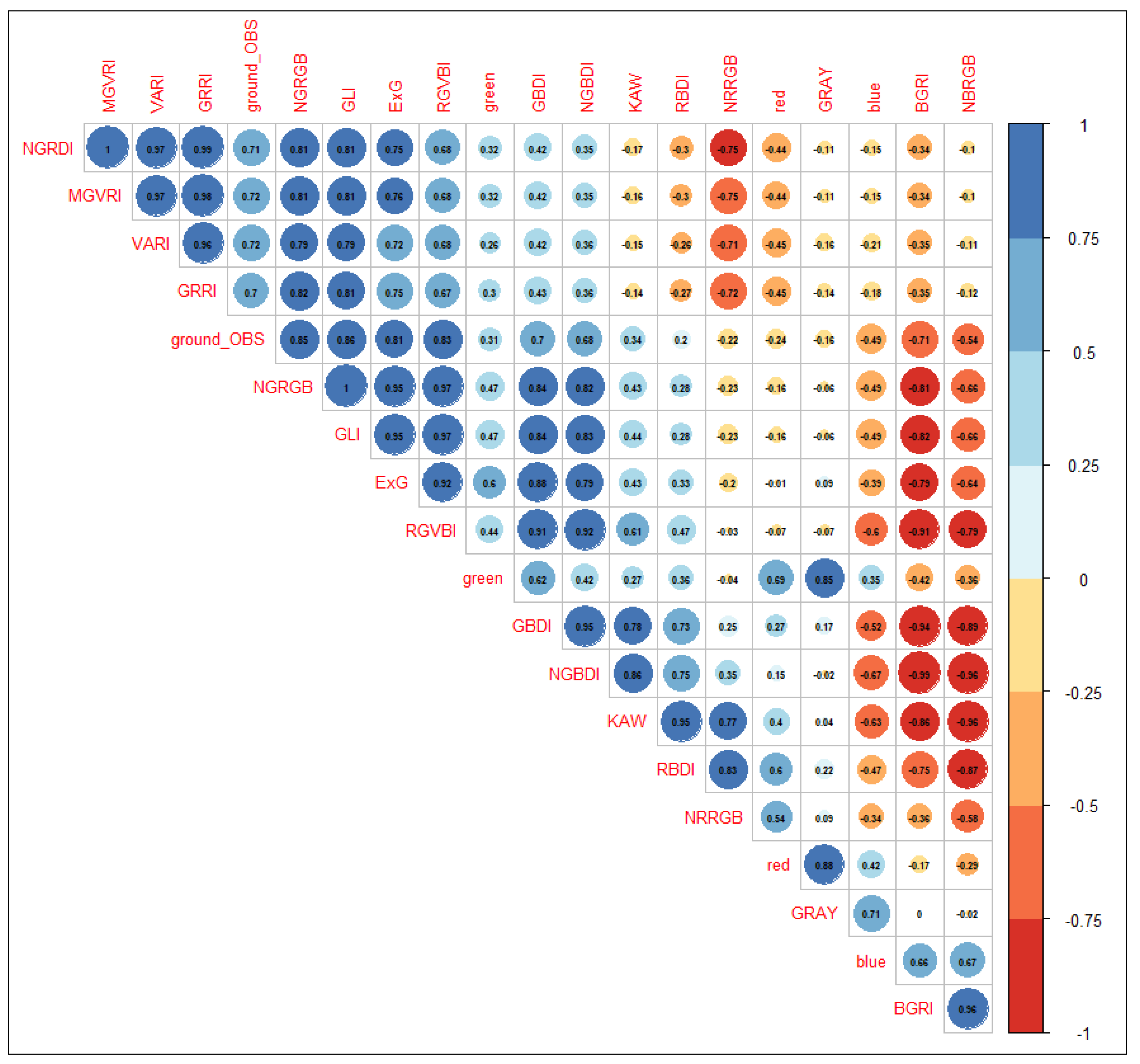
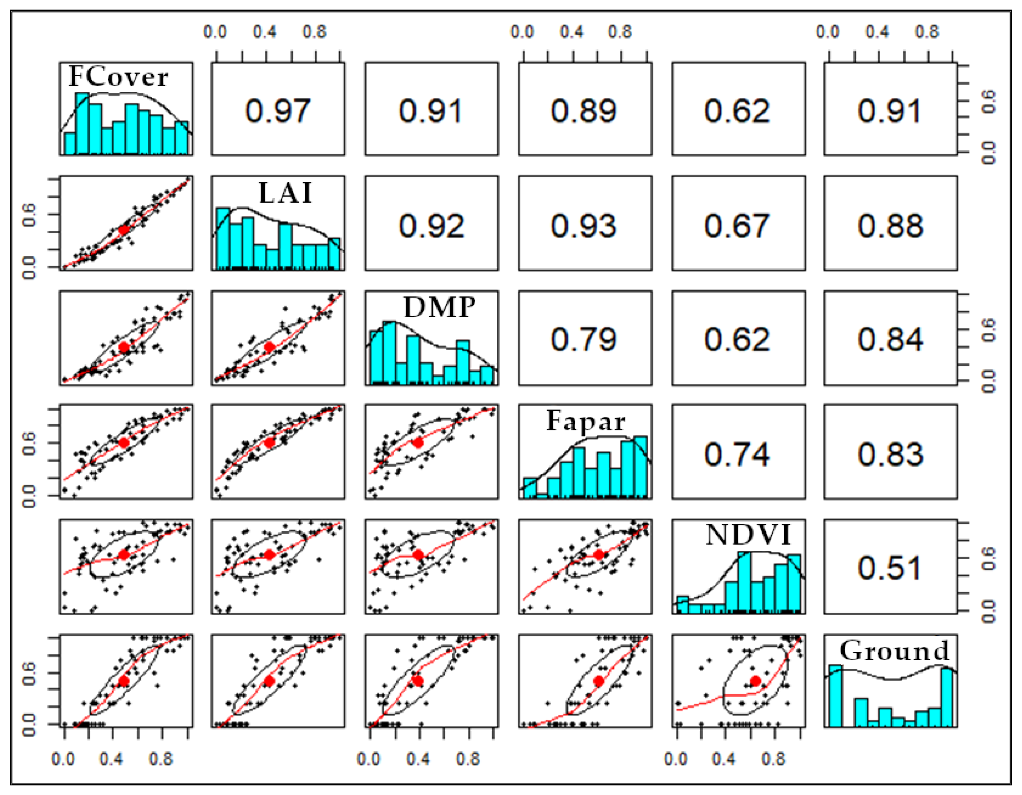
2.5.1. Correlation Analysis

The relation between the observed time series phenological stages collected from ground observations as percentages of the leaf cover and the estimated percentages of the leaf cover from the aerial images by human interpretation were analyzed using a correlation indicator. The same indicator was used to assess the correlation between the observed time series leaf cover and the VI values estimated for each tree. The corr function of the stats package in R [45] was used to compute the Pearson correlation method between the different time series data.
The corrplot R package [45] was used to provide a visual correlation matrix to detect patterns among variables and to test the null hypothesis that the true correlation coefficient ρ is equal to 0.

2.5.2. Regression Analysis

In order to predict the phenology stages as leaf cover, regression analysis was used. The goal was to find an algorithm or function which takes pixel values from either image from UAVs or the Copernicus biophysical parameters and outputs a response that is as close to the actual value of the phenology stages observed on the ground. Three error metrics were estimated to evaluate and report the performance of a regression model. The Mean Squared Error (MSE) refers to minimizing the mean squared error between predictions and expected values; the Root Squared Error (RMSE) is used as an extension of the MSE that matches the units of the target values and R-squared (R2), which represent the proportion of the variance in the dependent variable that explains the model.

Prediction of the Phenology Using Linear Regression Analysis

Two approaches were used to build a straightforward, reproducible model that predicted the phenology. The first model predicts the phenology as leaf coverage at the tree level based on the VIs calculated from UAV-collected images and location and time data predictors. The location was used as a site classifier, and the date was used to add seasonality to the prediction algorithm. In the second model, we aimed to predict a mean value per site based on the biophysical parameters collected from the Copernicus land monitoring service. Multiple regression models were tested to identify the most suitable predictors as well as the interaction between the them.

Prediction of the Phenology Using Non-Linear Regression Analysis

We implemented a random forest machine learning algorithm to predict the phenological stages at the tree level from aerial images. This algorithm uses random samples from observations and builds a model for which it measures a gain function and repeats the process k times to maximize the function. In this case, the non-linear regression algorithm operates by constructing decision trees based on the training dataset, which generates outcomes based on mean prediction.
Before starting the processing, the variable data series were rescaled to obtain values between 0 and 1, and time seasonality was added as a predictor. The machine learning algorithm was implemented using the caret package of the R software [45] by building the model on the training set (80% of data measuring 48 trees) and evaluating its performance on the test set (12 trees).

3. Results

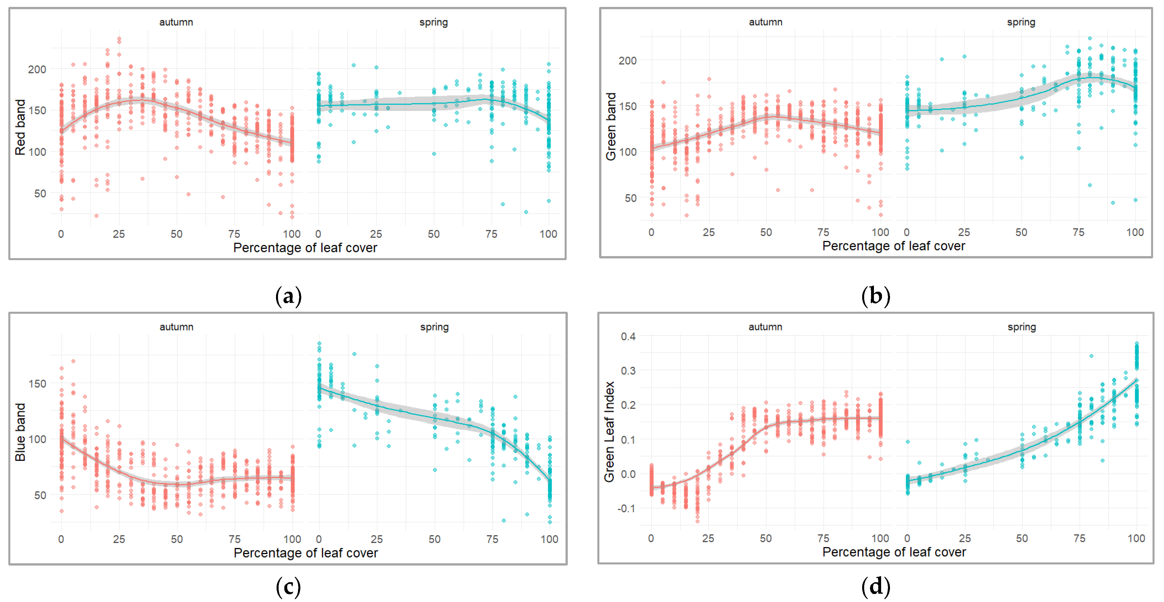
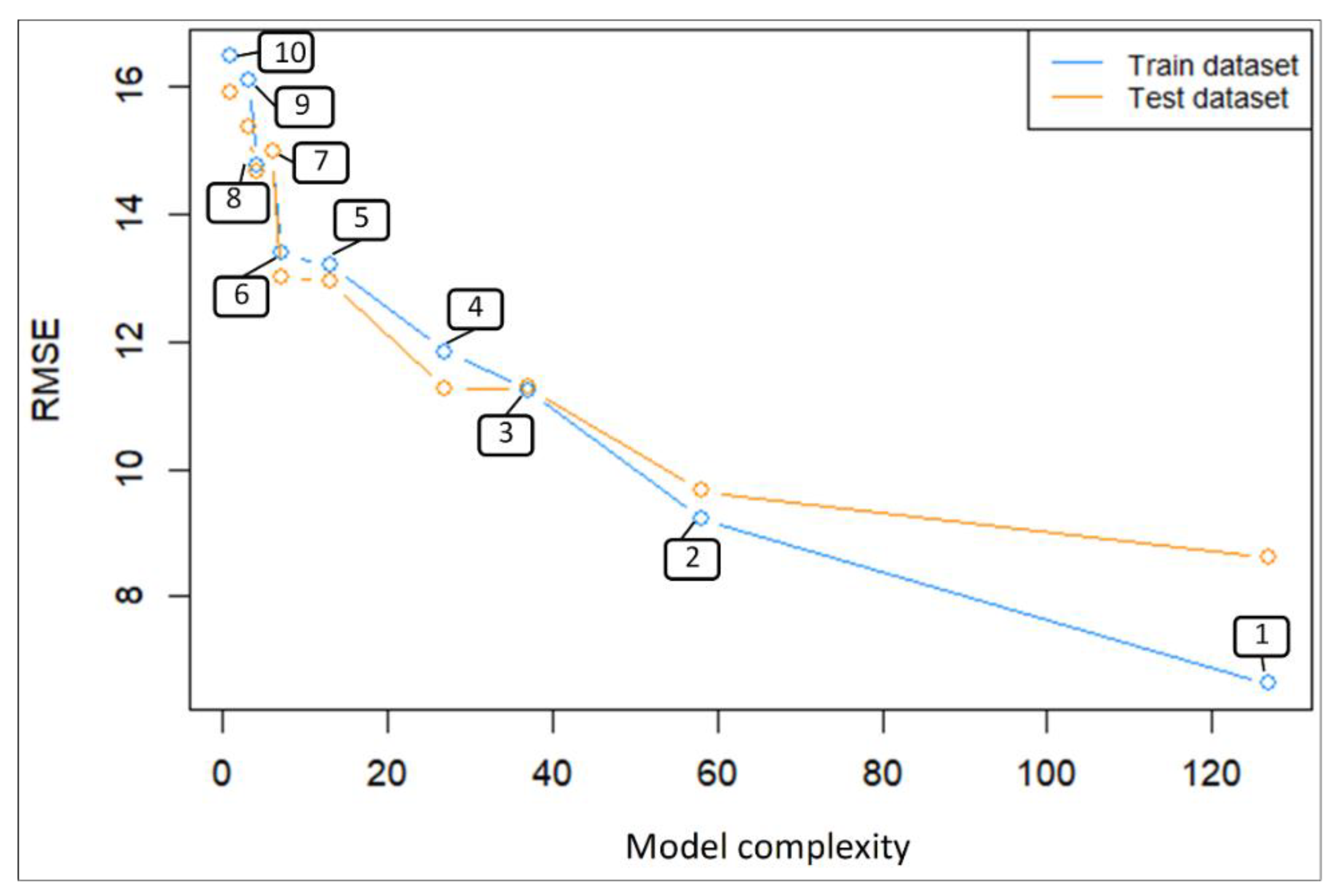
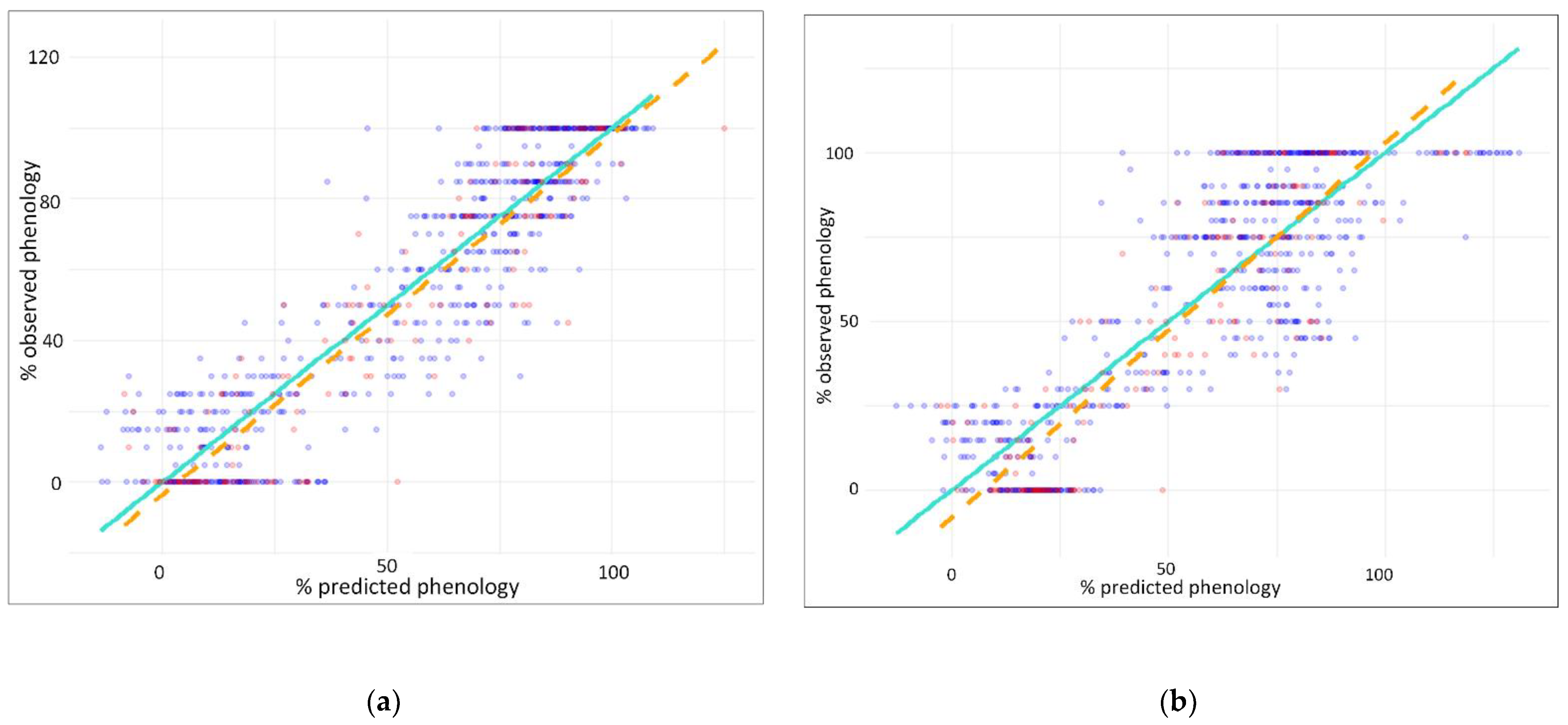
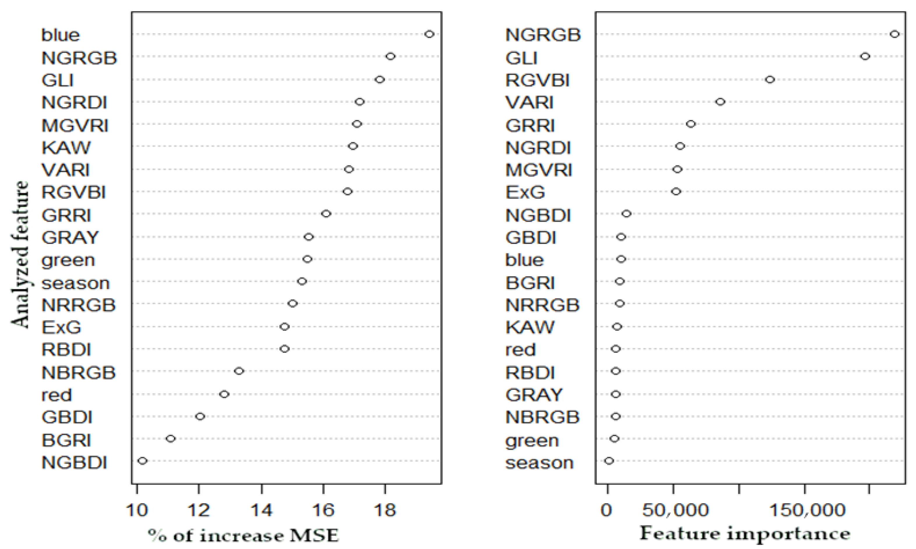
3.1. Predicting Leaf Phenology Using Aerial Images Collected by UAV

Based on the orthorectified aerial imagery collected from the UAV for each of the 60 individual trees in Sites 2 and 3, LU and senescence were estimated as a percentage of leaf cover by experts who were not involved in the ground observations. The values of the Pearson correlation coefficient between the ground phenology observations described by the scale in Table 2 and the leaf cover from the aerial observations were very high (r = 0.98).
For each tree, we retrieved the pixel values of the red, green, and blue band lengths contained inside a crown boundary along the growing season (Figure 3), calculated the VIs (Table 2), and recorded values as mean, median and standard error, which resulted in 864 observations × 50 predictors. All the Pearson correlation values estimated between the ground observations and the VIs used are presented in Appendix A Figure A3. Correlogram of the Pearson correlation between vegetation indices and ground leaf phenology observations. The numbers and the color gradient scale reveal the Pearson correlation value, and the size of the circle indicates the significance of the probability of the null hypothesis.
Four VIs show strong relation with leaf cover percentage during the entire growing season, resulting in correlation values above 0.8: GLI (0.86), NGRGB (0.85), RGVBI (0.83), and ExG (0.81), and five values more than 0.7: MGVRI (0.73), VARI (0.73), NGRDI (0.72), GRRI (0.71), and GBDI (0.70), which indicated a strong relationship.
Based on the relationship of the VIs with the ground observations, several linear regression models were fitted to predict the leaf phenology. In order to choose the best model, the performance was tested in both training and test data against the model complexity shown in Figure 4.
The model results are summarized in Table 5, showing the values of RMSE against the complexity and the linear model formula. Although the first model displayed a minor error, it had the highest complexity and overfitting tendency toward the leaf percentage prediction. Model ten, which was based on the best-performing VIs parameter alone, thus making it the least flexible, had a more significant error of 16% between the difference in leaf cover prediction and the actual data. Model three had appropriate RMSE values for both the training and test dataset; thus, we believe this model will display the best prediction on future datasets.
The predicted percentage of leaf cover versus the percentage observed on the ground is shown in the columns of both the trained and tested datasets’ RMSEs. The balance between the two dataset errors describes the model’s capacity to predict unseen data.
The comparison between model three, which shows an equal error in both datasets, and model ten, which is the simplest applicable model, is indicated in the scatterplot of the predicted leaf phenology versus the actual ground observations between both training and test datasets Figure 5.
A random forest regression algorithm was trained to perform a regression model to overcome the linear model’s limitations. It was based on all the statistical measurements (mean, median, and standard error) of the VIs and the time in the vegetation season. The model showed very good results; it explained 91.1% of the variance. The estimated performance metrics indicated a tendency to overfit on the train data, but a small overall error of 8% was reported in terms of the prediction of the percentage of leaf cover (Table 6).
The variable’s importance in defining the model performance and its influence on the MSE is shown in Figure 6.
A visualization of the actual data (observed through ground observations) and the values of leaf phenology predicted using the random forest algorithm are shown in Figure 7. The red line denotes the actual data for both the training and test datasets, and the predicted data are shown for the training dataset in dark blue and the test dataset in light blue. The predicted training dataset was based on 80% of the monitored individuals (48 from 60); the phenology of the other individuals left (12) was estimated through a predicted test.

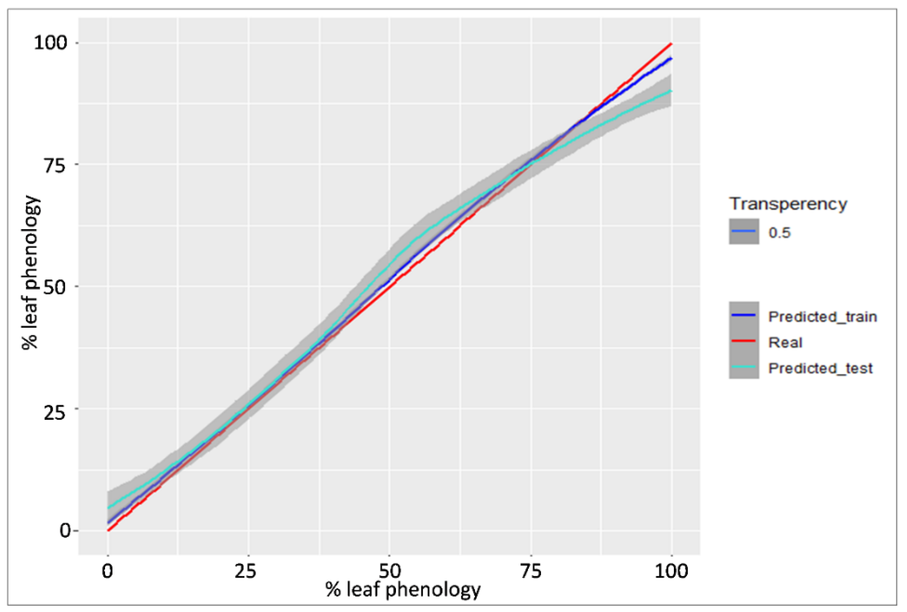
3.2. Predicting Leaf Phenology Using Copernicus Biophysical Parameters

For each of the five study sites (Table 1), the mean phenological phase for both LU and senescence was estimated during the entire growing season based on the ground observations.
Time series data collected from Copernicus biophysical parameters, such as mean values per site during the vegetation season, indicated a strong correlation between the four parameters and the phenological ground observations. The fraction of vegetation cover (FCover) index, which is based on the cover of green color of the vegetation from the ground (Table 4), was the most relevant and showed the strongest correlation with the phenological ground observations (r = 0.91). High correlation values between the time series data of the ground observations were also found compared to the LAI, DMP, and FAPAR parameters, with r = 0.88, r = 0.84, and r = 0.83, respectively (Appendix A Figure A4).
Due to the linear relation between the ground data and the Copernicus parameters, several linear models were fitted. The best-fitting model, i.e., the model with the smallest error, was model one, with a less than 8% error between the predicted leaf phenology as green cover and actual data on the ground. For this model, the location was used as an independent variable as a site classifier. In the other models, the location was not used as a parameter; thus, although they resulted in a higher error, they would more effectively predict leaf phenology on Fagus species outside the studied sites. The best trade-off between the RMSE and the model complexity was exhibited in model three, in which four of the Copernicus biophysical parameters and season interaction were used (Table 7).

4. Discussion

In this study, we aimed to identify means of measuring the phenology of the European beech species at a fine scale (individual trees) and the average values of the site locations. We used affordable—in terms of price—RGB sensors to extend the tree phenology observations, especially in rough terrain, mounted on UAV devices for phenology observations of individual trees, and we used geospatial products derived from satellite imagery (biophysical parameters from Copernicus Land Monitoring Service) to observe the mean site phenology. Both approaches showed promising results, which may be useful in phenological observations.
Visual observations of leaf phenology based on UAV images through human interpretation showed promising results compared with ground observations. The high correlation values between the time series datasets (r = 0.98) indicate that aerial images can offer a crown-level overview similar to below-canopy observations [4,10]. However, individual tree canopy observations based on aerial images depend on the forest structure and terrain topography, and these types of observations have limitations, especially in dense canopy structures, where the uncertainty of individual tree delineation is high at the margin boundary. As in this study, observations at the top of the canopy will ensure a satisfactory assessment of leaf phenology. Other aspects regarding the grade of human interpretation are the geometric accuracy and ground sample distance of the ortho-photo, which may affect the interpretation, especially in the first bud-burst stages when a smaller sample size pixel will ensure better assessment accuracy. Both human interpretation and VIs are affected by the quality of the ortho-photo mosaic, such as shaded areas and higher reflectance spots due to differences in light reflection angles [22]. Some of these issues were controlled through the acquisition workflow, e.g., by ensuring similar light conditions, using the same camera orientations with the sunlight angle, or identifying and removing the shaded areas during the workflow processing of the images.
Computations of the images’ red, green, and blue band length values captured during the vegetation season by the UAV sensor resulted in the 19 VIs (Table 3) commonly used to monitor vegetation biological processes [21,22]. Strong relationships were revealed between four VIs and ground observations, resulting in Pearson correlation values higher than 0.8. The Green Leaf Index (GLI index) obtained the highest r-value, 0.86, followed by the normalized green of RGB index (NGRGB), Reed Green Blue Vegetation index (RGVBI), and the excess of the green index (ExG). The NGRGB index, also known as the Green Chromatic Coordinate index, is most frequently used to study tree phenology [1,4,10,13,16,20], and this study showed a high correlation r-value of 0.85 with ground observations. Notably, the VI’s, with high correlation results, was based on the calculations of all three bands. This, of course, is related to the biophysical properties of each band; green and red bands are correlated with spring and autumn [3], respectively, and the blue band, which is a chlorophyll absorption band [10], provides variability in leaf phenology changes in both seasons (Figure 3). Other VIs have been identified in phenology vegetation studies, e.g., good results were obtained regarding barley leaves [21] with GBDI and ExG VIs, while the study of grass vegetation using RGB sensors [22] revealed the good performance of the NGDRI and MGVRI indices, estimated from aerial images. The NGRGB indices also showed accurate phenology observation comparisons between ground, UAV images, and satellite VIs [16,46]. Most studies that monitor vegetation based on UAV images use the Normalized Difference Vegetation Index (NDVI), the standard remote sensing indices [47]. As the NDVI application range is well known, its usage is constrained by the camera sensor’s capabilities to capture near-infrared light (NIR). In contrast, we used a standard affordable RGB sensor in this study. The use of the GLI and ExG indices in a study that aimed to perform object segmentation, trying to delimit the target objects from a residual background (agriculture field), showed that both are very accurate, with the latter displaying a slight advantage [48]. In addition to the quality of the segmentation performance of the target objects (masking off the ground and shadows and removing these values from the calculations), the different resolutions of the images collected at the time of the overflights also influence the quality of the images so in that case, a vegetation index may or may not have higher accuracy. For example, for UAV images acquired at an altitude of 6 m, the highest accuracy was shown by red and green indices, but when UAV images were acquired at an altitude of 50 m, the Green Blue Difference Index (GBDI) and the excess the green index (ExG) showed the highest accuracy [21]. In our case, when UAV images were acquired at an altitude of 150 m to overcome the site’s irregular topography, the highest accuracy was shown by the GLI indices.
The calculated average values of the crown VIs pixels may not be enough to describe the leaf phenology at the individual level [10], as they do not achieve similar results in different illumination conditions. Due to the different light conditions during the flights, the light angle, and land topography, the precision of leaf phenology estimation may decrease [22,49]. The standard deviation of pixel values described the variation in the color and shadows in the high pixel resolution used in this study.
The correlation analysis between the ground observations and time series VIs was further used to build and test a predicting algorithm for leaf phenology as a percentage of leaf cover. Deterministic models, such as linear regression, and non-deterministic models, random forest algorithms, were tested to predict the percentage of the leaf cover against data collected from the ground. The linear regression model is more practical and can more easily replicate the prediction of leaf phenology in other European beach sites. However, its complexity increases to enable a minor error percentage. This trade-off between the model complexity and RMSE (Figure 4) was observed in both the training and test datasets. This computation indicates that a more complex model will also be more capable of predicting the percentage of the leaf phenology but with a tendency to overfit, meaning it has a lower prediction capability than other sites. By comparing the RMSE in both the training and test datasets, we observed that model number three (Table 5) displayed the most appropriate level of error and was thus identified as the most versatile model. Model three used all the VIs with correlations above r = 0.8 as the mean, median, and standard error of the sampled crown pixels, along with season interaction. The inclusion of the season-independent variable indicated a strong relationship between the prediction capabilities in the vegetation season. The mean RMSE of 11% leaf coverage between the predicted and actual values indicated a good predicting capability of the model identified to be the best fitted.
An increased prediction capability with a minor RMSE was obtained using a random forest algorithm based on the VIs extracted from aerial images and vegetation season. The algorithm predicted the percentage of leaf cover in the training dataset with a minimal error (RMSE = 3%, Table 6) but slightly higher in the test dataset (RMSE = 8%). These results indicate an overfitting tendency for predicting, which was shown by comparing the RMSE of the training and test datasets (Table 6), also influenced by the small sample size dataset used to train the algorithm. While the fitted line between predicted and actual values in the training data were similar to the percentage of leaf cover in the trial dataset, the algorithm overestimated the percentage of leaf cover at 0–75% intervals. It underestimated the remaining to 100% intervals. The satisfactory results of the machine learning algorithms increased the possibility of applying them to other trees’ biological and ecological processes collected from remote sensing [10] by linking them to the information collected from the ground. Good predictive accuracy of the random forest algorithm was also revealed by studying the flowering of Eucalyptus species from metrics collected from RGB sensors [50], as well as linking carotenoid-sensitive spectral indices to track the phenology in conifers [51].
In our study, the human interpretation of the leaf phenology on the ground and based on UAV images showed a high correlation and could be used for cross-validation. The high correlation between the VIs and data collected from the ground, along with the good prediction capabilities, shows that UAV image analysis can extend phenology studies and cover large areas which can be used to validate ecosystem processes [1]. The results, which are also similar to other studies [5], show the capability of UAV sensors to characterize crown-level phenology at fine spatial and temporal scales and describe the variability in forest landscapes [3]. In future studies of leaf phenology prediction, modeling limitations will need to be addressed. The number of sampled trees should be increased to improve the training of the algorithm and use a digital image analyzer for the canopy on the ground to calibrate the model.
Nevertheless, visual assessment can be complex in a highly dense crown covered with an additional understory. Further site analysis of individual trees will be needed to train linear and random forest regression algorithms. Despite the promising results regarding phenology observation using an RGB sensor mounted on a UAV, the method is restrictive in terms of the area and time of the observation. The coverage area per flight is between 20 and 30 ha for a GSD between 4 and 8 cm (using this study flight parameter), and the atmospheric restrictions include sufficient light conditions (brightness and angle of reflectance), lack of rain, and low wind speed.
The biophysical parameters available in the Copernicus land monitoring platform at ten-day intervals monitor the vegetation phenology and the productivity of ecosystem habitats. Measuring the phenology of individual trees at high resolution on both spatial and temporal levels, although offering valuable information in understanding the ecological component affecting a tree’s biological processes, may be limited to the study of small-scale ecological processes. The overall phenological process cycle at each site is recorded using satellite imagery [16]. To overcome and expand the study, we investigated the relationship between the site mean percentage of leaf cover from ground observation data and the biophysical parameters estimated from satellite imagery of the Copernicus program. Correlation analysis of the time series between the data collected from the ground describing the mean percentage of leaf cover and the five satellite-based biophysical parameter values (Table 6) showed correlation values r < 0.5 (Figure 5). The fraction of vegetation cover (FCover) obtained the highest value (0.91), proving it had the strongest correlation with the phenological observations from the ground. The FCover indices quantify the spatial extent of the green vegetation [19], being independent of the illumination direction, which can be a candidate to replace classical VIs for monitoring ecosystems. The strong correlation between the chlorophyll content and spectral indices of European beech trees [25] may indicate the good relation between the FCover and leaf phenology. In terms of the correlation results, this was followed by the Leaf Area Index (0.88), dry matter productivity (0.84), and a fraction of absorbed photosynthetically active radiation (0.81); the last one, the Normalized Difference Vegetation Index (NDVI), only obtained a correlation of 0.51. It may be possible to upscale the phenology observations through ground or UAV observations; in addition, studies have shown high correlations by comparing VIs based on satellite and near-surface sensors [13]. The NDVI indices acted poorly when monitoring the phenology of the European beech along an altitudinal gradient in Slovakia [52], as significant differences in the leaf onset and the end of leaf onset was not identified with phenological metrics derived from the NDVI, extracted from the Moderate Resolution Imaging Spectroradiometer satellite (MODIS).

5. Conclusions

Using images collected from UAVs, biological functions such as seasonal changes in phenology can be observed at the individual tree level in relatively large areas of study. The maps produced using aerial images offer a good overview of the tree crown, comparable with the observation from the ground. They can be used, with excellent accuracy, for visual observations of leaf phenology. The VIs calculated from these images significantly relate to the leaf phenology observations from the ground throughout the growing season. Overall, UAV observations can drastically reduce the effort needed to undertake phenology observations. The VIs with high correlations, such as values above 0.8 (GLI, NGRGB, RGVBI, and ExG), use all three bands (red, green, and blue) of the RGB sensor in their calculations, as all of the bands can track different phenological stages during the growing season. Prediction models show good accuracy using random forest machine learning algorithms, whereas, on small testing datasets (sites), they tend to overfit the data and thus not produce the same results in a new site study. Although the RMSE in the test dataset was 8%, further analysis should be performed to obtain a robust algorithm. A satisfactory result was also obtained using a linear model based on the VIs. The algorithms showed higher accuracy in both cases when both color and texture metrics were used as independent variables.
The biophysical parameters based on Sentinel satellites, available on the Copernicus land monitoring platform, generally showed satisfactory accuracy in the prediction of an average site value of the percentage of leaf cover. Significantly, the fraction of vegetation cover (FCover) index showed the strongest correlation with the ground observations of leaf phenology.

Author Contributions

Conceptualization, G.R.R., M.I.C.C. and A.L.C.; methodology, M.I.C.C. and G.R.R.; software, G.R.R.; validation, M.I.C.C. and G.R.R.; formal analysis, G.R.R.; resources, G.R.R.; writing—original draft preparation, M.I.C.C.; writing—review and editing, M.I.C.C., G.R.R. and A.L.C.; supervision, A.L.C.; funding acquisition, A.L.C., G.R.R. All authors have read and agreed to the published version of the manuscript.

Funding

This research received no external funding. The APC was funded by the “Transilvania” University of Brasov and the Marin Drăcea” National Institute for Research and Development in Forestry.

Data Availability Statement

The data presented in this study are available on request from the corresponding author.

Acknowledgments

The authors thank the members of the forest monitoring team from the “Marin Drăcea” National Institute for Research and Development in Forestry, Department of Forest Management, Romania, for their help in providing the equipment for the collection of data.

Conflicts of Interest

The authors declare no conflict of interest.

Appendix A

Appendix A.1. Image Collecting and Processing

Figure A1. The monitored trees in sites two and three; are represented in a topographic map (Google satellite as baseline) and the Digital Terrain Model (DSM) resulting from the mosaic of images collected by UAV.
Remotesensing 14 06198 g0a1
Figure A2. Example of images along the growing season timescale before (a) and after (b) removing shadows and changing the digital values of pixels to non-value. Dashed magenta regions represented crown delineation and were used to retrieve the RGB band length values.
Remotesensing 14 06198 g0a2

Appendix A.2. Correlation Analysis

Figure A3. Correlogram of the Pearson correlation between vegetation indices and ground leaf phenology observations. The numbers and the color gradient scale reveal the Pearson correlation value, and the size of the circle indicates the significance of the probability of the null hypothesis.
Remotesensing 14 06198 g0a3
Figure A4. Correlation analysis between Copernicus biophysical parameters and the mean phenological phase of each study site.
Remotesensing 14 06198 g0a4

References

  1. Klosterman, S.; Melaas, E.; Wang, J.A.; Martinez, A.; Frederick, S.; O’Keefe, J.; Orwig, D.A.; Wang, Z.; Sun, Q.; Schaaf, C.; et al. Fine-Scale Perspectives on Landscape Phenology from Unmanned Aerial Vehicle (UAV) Photography. Agric. For. Meteorol. 2018, 248, 397–407. [Google Scholar] [CrossRef]
  2. Xie, Y.; Civco, D.L.; Silander, J.A., Jr. Species-Specific Spring and Autumn Leaf Phenology Captured by Time-Lapse Digital Cameras. Ecosphere 2018, 9, e02089. [Google Scholar] [CrossRef] [Green Version]
  3. Klosterman, S.; Richardson, A.D. Observing Spring and Fall Phenology in a Deciduous Forest with Aerial Drone Imagery. Sensors 2017, 17, 2852. [Google Scholar] [CrossRef] [PubMed] [Green Version]
  4. Atkins, J.W.; Stovall, A.E.L.; Yang, X. Mapping Temperate Forest Phenology Using Tower, UAV, and Ground-Based Sensors. Drones 2020, 4, 56. [Google Scholar] [CrossRef]
  5. Fawcett, D.; Bennie, J.; Anderson, K. Monitoring Spring Phenology of Individual Tree Crowns Using Drone-Acquired NDVI Data. Remote Sens. Ecol. Conserv. 2021, 7, 227–244. [Google Scholar] [CrossRef]
  6. Twardosz, R.; Walanus, A.; Guzik, I. Warming in Europe: Recent Trends in Annual and Seasonal Temperatures. Pure Appl. Geophys. 2021, 178, 4021–4032. [Google Scholar] [CrossRef]
  7. Aitken, S.N.; Yeaman, S.; Holliday, J.A.; Wang, T.; Curtis-McLane, S. Adaptation, Migration or Extirpation: Climate Change Outcomes for Tree Populations. Evol. Appl. 2008, 1, 95–111. [Google Scholar] [CrossRef]
  8. Scranton, K.; Amarasekare, P. Predicting Phenological Shifts in a Changing Climate. Proc. Natl. Acad. Sci. USA 2017, 114, 13212–13217. [Google Scholar] [CrossRef] [Green Version]
  9. Weisberg, P.J.; Dilts, T.E.; Greenberg, J.A.; Johnson, K.N.; Pai, H.; Sladek, C.; Kratt, C.; Tyler, S.W.; Ready, A. Phenology-Based Classification of Invasive Annual Grasses to the Species Level. Remote Sens. Environ. 2021, 263, 112568. [Google Scholar] [CrossRef]
  10. Park, J.Y.; Muller-Landau, H.C.; Lichstein, J.W.; Rifai, S.W.; Dandois, J.P.; Bohlman, S.A. Quantifying Leaf Phenology of Individual Trees and Species in a Tropical Forest Using Unmanned Aerial Vehicle (UAV) Images. Remote Sens. 2019, 11, 1534. [Google Scholar] [CrossRef]
  11. Budeanu, M.; Petritan, A.M.; Popescu, F.; Vasile, D.; Tudose, N.C. The Resistance of European Beech (Fagus Sylvatica) From the Eastern Natural Limit of Species to Climate Change. Not. Bot. Horti Agrobot. Cluj-Napoca 2016, 44, 625–633. [Google Scholar] [CrossRef] [Green Version]
  12. Chesnoiu, E.N.; Șofletea, N.; Curtu, A.L.; Toader, A.; Radu, R.; Enescu, M. Bud Burst and Flowering Phenology in a Mixed Oak Forest from Eastern Romania. Ann. For. Res. 2009, 52, 199–206. [Google Scholar] [CrossRef]
  13. Thapa, S.; Garcia Millan, V.E.; Eklundh, L. Assessing Forest Phenology: A Multi-Scale Comparison of Near-Surface (UAV, Spectral Reflectance Sensor, PhenoCam) and Satellite (MODIS, Sentinel-2) Remote Sensing. Remote Sens. 2021, 13, 1597. [Google Scholar] [CrossRef]
  14. Sánchez-Azofeifa, A.; Rivard, B.; Wright, J.; Feng, J.-L.; Li, P.; Chong, M.M.; Bohlman, S.A. Estimation of the Distribution of Tabebuia Guayacan (Bignoniaceae) Using High-Resolution Remote Sensing Imagery. Sensors 2011, 11, 3831–3851. [Google Scholar] [CrossRef]
  15. Lopes, A.P.; Nelson, B.W.; Wu, J.; de Graça, P.M.L.A.; Tavares, J.V.; Prohaska, N.; Martins, G.A.; Saleska, S.R. Leaf Flush Drives Dry Season Green-up of the Central Amazon. Remote Sens. Environ. 2016, 182, 90–98. [Google Scholar] [CrossRef]
  16. Berra, E.F.; Gaulton, R.; Barr, S. Assessing Spring Phenology of a Temperate Woodland: A Multiscale Comparison of Ground, Unmanned Aerial Vehicle and Landsat Satellite Observations. Remote Sens. Environ. 2019, 223, 229–242. [Google Scholar] [CrossRef]
  17. Budianti, N.; Mizunaga, H.; Iio, A. Crown Structure Explains the Discrepancy in Leaf Phenology Metrics Derived from Ground- and UAV-Based Observations in a Japanese Cool Temperate Deciduous Forest. Forests 2021, 12, 425. [Google Scholar] [CrossRef]
  18. Gray, R.E.J.; Ewers, R.M. Monitoring Forest Phenology in a Changing World. Forests 2021, 12, 297. [Google Scholar] [CrossRef]
  19. Fuster, B.; Sánchez-Zapero, J.; Camacho, F.; García-Santos, V.; Verger, A.; Lacaze, R.; Weiss, M.; Baret, F.; Smets, B. Quality Assessment of PROBA-V LAI, FAPAR and FCOVER Collection 300 m Products of Copernicus Global Land Service. Remote Sens. 2020, 12, 1017. [Google Scholar] [CrossRef] [Green Version]
  20. Wu, S.; Wang, J.; Yan, Z.; Song, G.; Chen, Y.; Ma, Q.; Deng, M.; Wu, Y.; Zhao, Y.; Guo, Z.; et al. Monitoring Tree-Crown Scale Autumn Leaf Phenology in a Temperate Forest with an Integration of PlanetScope and Drone Remote Sensing Observations. ISPRS J. Photogramm. Remote Sens. 2021, 171, 36–48. [Google Scholar] [CrossRef]
  21. Liu, Y.; Hatou, K.; Aihara, T.; Kurose, S.; Akiyama, T.; Kohno, Y.; Lu, S.; Omasa, K. A Robust Vegetation Index Based on Different UAV RGB Images to Estimate SPAD Values of Naked Barley Leaves. Remote Sens. 2021, 13, 686. [Google Scholar] [CrossRef]
  22. Barbosa, B.D.S.; Ferraz, G.A.S.; Gonçalves, L.M.; Marin, D.B.; Maciel, D.T.; Ferraz, P.F.P.; Rossi, G. RGB Vegetation Indices Applied to Grass Monitoring: A Qualitative Analysis. Agron. Res. 2019, 17, 349–357. [Google Scholar] [CrossRef]
  23. Kawashima, S.; Nakatani, M. An Algorithm for Estimating Chlorophyll Content in Leaves Using a Video Camera. Ann. Bot. 1998, 81, 49–54. [Google Scholar] [CrossRef] [Green Version]
  24. Wang, Y.; Wang, D.; Shi, P.; Omasa, K. Estimating Rice Chlorophyll Content and Leaf Nitrogen Concentration with a Digital Still Color Camera under Natural Light. Plant Methods 2014, 10, 36. [Google Scholar] [CrossRef] [Green Version]
  25. Morley, P.J.; Jump, A.S.; West, M.D.; Donoghue, D.N.M. Spectral Response of Chlorophyll Content during Leaf Senescence in European Beech Trees. Environ. Res. Commun. 2020, 2, 071002. [Google Scholar] [CrossRef]
  26. Gitelson, A.A.; Kaufman, Y.J.; Stark, R.; Rundquist, D. Novel Algorithms for Remote Estimation of Vegetation Fraction. Remote Sens. Environ. 2002, 80, 76–87. [Google Scholar] [CrossRef] [Green Version]
  27. Geßler, A.; Keitel, C.; Kreuzwieser, J.; Matyssek, R.; Seiler, W.; Rennenberg, H. Potential Risks for European Beech (Fagus Sylvatica L.) in a Changing Climate. Trees 2007, 21, 1–11. [Google Scholar] [CrossRef]
  28. Zlatník: Lesnická Fytocenologie: Příručka Pro...—Google Scholar. Available online: https://scholar.google.com/scholar_lookup?title=Lesnick%C3%A1%20fytocenologie&publication_year=1978&author=Zlatn%C3%ADk%2CA. (accessed on 13 October 2022).
  29. Schieber, B. Spring Phenology of European Beech (Fagus Sylvatica L.) in a Submountain Beech Stand with Different Stocking in 1995–2004. J. For. Sci. 2006, 52, 208–216. [Google Scholar] [CrossRef] [Green Version]
  30. Leuschner, C. Drought Response of European Beech (Fagus Sylvatica L.)—A Review. Perspect. Plant Ecol. Evol. Syst. 2020, 47, 125576. [Google Scholar] [CrossRef]
  31. Vitasse, Y.; Delzon, S.; Dufrêne, E.; Pontailler, J.-Y.; Louvet, J.-M.; Kremer, A.; Michalet, R. Leaf Phenology Sensitivity to Temperature in European Trees: Do within-Species Populations Exhibit Similar Responses? Agric. For. Meteorol. 2009, 149, 735–744. [Google Scholar] [CrossRef]
  32. Alberto, F.; Bouffier, L.; Louvet, J.-M.; Lamy, J.-B.; Delzon, S.; Kremer, A. Adaptive Responses for Seed and Leaf Phenology in Natural Populations of Sessile Oak along an Altitudinal Gradient. J. Evol. Biol. 2011, 24, 1442–1454. [Google Scholar] [CrossRef]
  33. PIX4Dmapper: Professional Photogrammetry Software for Drone Mapping. Available online: https://www.pix4d.com/product/pix4dmapper-photogrammetry-software (accessed on 26 November 2022).
  34. OpenDroneMap. WebODM: Drone Mapping Software (Version 1.1.0). Available online: https://www.opendronemap.org/webodm/ (accessed on 1 March 2021).
  35. QGIS. QGIS Project 3.26.3. 2017. Available online: https://www.qgis.org/nl/site/ (accessed on 1 March 2021).
  36. Pearson, R.L.; Miller, L.D.; Tucker, C.J. Hand-Held Spectral Radiometer to Estimate Gramineous Biomass. Appl. Opt. 1976, 15, 416–418. [Google Scholar] [CrossRef]
  37. Fuentes, D.A.; Gamon, J.A.; Qiu, H.; Sims, D.A.; Roberts, D.A. Mapping Canadian Boreal Forest Vegetation Using Pigment and Water Absorption Features Derived from the AVIRIS Sensor. J. Geophys. Res. Atmos. 2001, 106, 33565–33577. [Google Scholar] [CrossRef] [Green Version]
  38. Zarco-Tejada, P.J.; Berjón, A.; López-Lozano, R.; Miller, J.R.; Martín, P.; Cachorro, V.; González, M.R.; de Frutos, A. Assessing Vineyard Condition with Hyperspectral Indices: Leaf and Canopy Reflectance Simulation in a Row-Structured Discontinuous Canopy. Remote Sens. Environ. 2005, 99, 271–287. [Google Scholar] [CrossRef]
  39. Woebbecke, D.M.; Meyer, G.E.; Von Bargen, K.; Mortensen, D.A. Color Indices for Weed Identification Under Various Soil, Residue, and Lighting Conditions. Trans. ASAE 1995, 38, 259–269. [Google Scholar] [CrossRef]
  40. Rouse, J.W.; Haas, R.H.; Schell, J.A.; Deering, D.W. Monitoring Vegetation Systems in the Great Plains with ERTS. Nasa Spec. Publ. 1974, 351, 309. [Google Scholar]
  41. Hunt, E.R.; Cavigelli, M.; Daughtry, C.S.T.; Mcmurtrey, J.E.; Walthall, C.L. Evaluation of Digital Photography from Model Aircraft for Remote Sensing of Crop Biomass and Nitrogen Status. Precis. Agric. 2005, 6, 359–378. [Google Scholar] [CrossRef]
  42. Louhaichi, M.; Borman, M.M.; Johnson, D.E. Spatially Located Platform and Aerial Photography for Documentation of Grazing Impacts on Wheat. Geocarto Int. 2001, 16, 65–70. [Google Scholar] [CrossRef]
  43. Bendig, J.; Yu, K.; Aasen, H.; Bolten, A.; Bennertz, S.; Broscheit, J.; Gnyp, M.L.; Bareth, G. Combining UAV-Based Plant Height from Crop Surface Models, Visible, and near Infrared Vegetation Indices for Biomass Monitoring in Barley. Int. J. Appl. Earth Obs. Geoinf. 2015, 39, 79–87. [Google Scholar] [CrossRef]
  44. Copernicus Land Monitoring Service. Available online: https://land.copernicus.eu/ (accessed on 13 March 2022).
  45. R Project for Statistical Computing. R Version 4.1.3, Released on 10.03.2022. Available online: https://www.r-project.org/ (accessed on 31 March 2022).
  46. Berra, E.F.; Gaulton, R.; Barr, S. Use of a Digital Camera Onboard a UAV to Monitor Spring Phenology at Individual Tree Level. In Proceedings of the 2016 IEEE International Geoscience and Remote Sensing Symposium (IGARSS), Beijing, China, 10–15 July 2016; pp. 3496–3499. [Google Scholar]
  47. Yengoh, G.T.; Dent, D.; Olsson, L.; Tengberg, A.E.; Tucker, C.J., III. Use of the Normalized Difference Vegetation Index (NDVI) to Assess Land Degradation at Multiple Scales: Current Status, Future Trends, and Practical Considerations; SpringerBriefs in Environmental Science; Springer International Publishing: Cham, Switzerland, 2016; ISBN 978-3-319-24110-4. [Google Scholar]
  48. Zhao, B.; Zhang, J.; Yang, C.; Zhou, G.; Ding, Y.; Shi, Y.; Zhang, D.; Xie, J.; Liao, Q. Rapeseed Seedling Stand Counting and Seeding Performance Evaluation at Two Early Growth Stages Based on Unmanned Aerial Vehicle Imagery. Front. Plant Sci. 2018, 9, 1362. [Google Scholar] [CrossRef]
  49. Bannari, A.; Guedon, A.M.; El Harti, A.; Cherkaoui, F.Z.; El-Ghmari, A.; Saquaque, A. Slight and Moderate Saline and Sodic Soils Characterization in Irrigated Agricultural Land Using Multispectral Remote Sensing. Int. Arch. Photogramm. Remote Sens. Spat. Inf. Sci. 2013, 34, 1–6. [Google Scholar]
  50. Dixon, D.J.; Callow, J.N.; Duncan, J.M.A.; Setterfield, S.A.; Pauli, N. Satellite Prediction of Forest Flowering Phenology. Remote Sens. Environ. 2021, 255, 112197. [Google Scholar] [CrossRef]
  51. D’Odorico, P.; Besik, A.; Wong, C.Y.S.; Isabel, N.; Ensminger, I. High-Throughput Drone-Based Remote Sensing Reliably Tracks Phenology in Thousands of Conifer Seedlings. New Phytol. 2020, 226, 1667–1681. [Google Scholar] [CrossRef]
  52. Lukasová, V.; Bucha, T.; Škvareninová, J.; Škvarenina, J. Validation and Application of European Beech Phenological Metrics Derived from MODIS Data along an Altitudinal Gradient. Forests 2019, 10, 60. [Google Scholar] [CrossRef]
Figure 1. Topographic map of the study area in Brasov region, and the five sites, red circles across the altitudinal gradient (left-hand corner map). Study sites are numbered following Table 1.
Remotesensing 14 06198 g001
Figure 2. Example of individual sampled beech trees captured at different phenological stages (month and day in the upper left corner of each image) using UAVs during the 2021 growing season. Dashed magenta regions represented crown delineation and were used to retrieve the RGB band length values.
Remotesensing 14 06198 g002
Figure 3. Relation between ground data observations, horizontal axis and (a) red, (b) green, and (c) blue spectral bands digital values, vertical axis, and (d) GLI among spring (blue color) and autumn (red color) seasons.
Remotesensing 14 06198 g003
Figure 4. The plot of models RMSE against model complexity on training and test dataset. Each number in the square represents the model number, as shown in Table 5.
Remotesensing 14 06198 g004
Figure 5. Compared performance between two linear models (a) model three and (b) model ten. The figure shows the relation between predicted (horizontal axis) versus actual phenology observation (vertical axis) between the training dataset (blue dots) and the test datasets (red dots). The fitted lines of the training data are in light blue, and the fitted line of the test data is in orange.
Remotesensing 14 06198 g005
Figure 6. The variable’s importance for each component is expressed as a percent of MSE in the random forest algorithm (left), and feature importance is expressed as an increase in node purity (right). Higher values reflect that variable has more importance in the model.
Remotesensing 14 06198 g006
Figure 7. Comparison of actual and predicted data on both training and test datasets.
Remotesensing 14 06198 g007
Table 1. Description of study sites.
NumberNameGeographic CoordinatesAltitude Range (Meters)Mean Temperature (°C) 1Mean Precipitation (Millimeters) 1
Site 1Ruia45°34′25.41″N
25°33′11.67″E
1300–14503.51023
Site 2Lupului45°34′54.64″N
25°32′36.43″E
1000–11505.2957
Site 3Solomon45°36′59.75″N
25°33′39.87″E
800–10006.2855
Site 4Tampa45°38′18.86″N
25°35′38.56″E
650–7507.2791
Site 5Lempes45°43′34.88″N
25°39′30.66″E
550–6107.5712
1 data extracted from WorldClim.
Table 2. Phenological stages linked to the observed percentage of leaf cover.
CodePhenological Stage
(3)
Range of the Percentage of Leaf Cover (%)
(2)
0Dormant winter bud<25
1Bud-swollen26–50
2Bud-burst51–75
3At least one leaf unfolding>75
Table 3. Estimated vegetation indices used in the analysis.
No.NameAbbreviationEquationReference
1Digital number for red bandRred/255[36]
2Digital number for green bandGgreen/255[36]
3Digital number for blue bandBblue/255[36]
4Green Red Ratio Index GRRIG/R[37]
5Blue Green Ratio IndexBGRIB/G[38]
6Green Blue Difference IndexGBDIG − B[23]
7Red Blue Difference IndexRBDIR − B[23]
8Excess of green indexExG2G − R − B[39]
9Grayscale IndexGRAY(R + G + B)/3[24]
10Chromatic coordinates for red/
Normalized red of RGB
NRRGBR/(R + G + B)[39]
11Chromatic coordinates for green/
Normalized green of RGB
NGRGBG/(R + G + B)[39]
12Chromatic coordinates for blue/
Normalized blue of RGB
NBRGBB/(R + G + B)[39]
13Normalized Green Red Difference IndexNGRDI(G − R)/(G + R)[40]
14Kawashima index KAW(R − B)/(R + B)[23]
15Normalized Green Blue Difference indexNGBDI(G − B)/(G + B)[41]
16Green Leaf IndexGLI(2G − R − B)/(2G + R + B)[42]
17Modified Green Red Vegetation IndexMGVRI(G2 − R2)/(G2 + R2)[43]
18Red Green Blue Vegetation Index RGVBI(G − B × R)/(G2 + B × R)[43]
19Visible Atmospherically Resistant
Index
VARI(G − R)/(G + R − B)[26]
Table 4. Copernicus biophysical parameters used to study leaf phenology.
No.NameAbbreviationDescription
1Dry Matter ProductivityDMPthe overall growth rate or dry biomass increase of the vegetation (kg/ha/day) [44]
2Fraction of Absorbed Photosynthetically Active RadiationFAPARquantifies the fraction of the solar radiation absorbed by live leaves for photosynthesis activity [44]
3Fraction of Vegetation CoverFCoverfraction of ground covered by green vegetation [44]
4Leaf Area IndexLAIhalf the total area of green elements of the canopy per unit of the horizontal ground area [44]
5Normalized Difference Vegetation IndexNDVIindicator of the greenness of the biomass [44]
Table 5. The summary of each of the model results. RMSE in both training and test datasets. The model complexity reveals the number of parameters, and the linear model formula is represented as a notation convention.
No.Train RMSETest RMSER2
Train Data
R2
Test Data
Model ComplexityIndependent Variable Component of the Linear Model Equation
16.638.610.940.901271 F(x) = NGRGB × GLI × ExG × RGVBI × GBDI × NGBDI × season
29.219.650.880.87581 F(x) = R + G + B + GRRI + BGRI + GBDI + RBDI + ExG + GRAY + NRRGB + NGRGB + NBRGB + NGRDI + KAW + NGBDI + GLI + MGVRI + RGVBI + VARI
311.2411.270.840.84372 F(x) = (NGRGB_m + NGRGB_me + NGRGB_sd + GLI_m + GLI_me + GLI_sd + ExG_m + ExG_me + ExG_sd + RGVBI_m + RGVBI_me + RGVBI_sd + GBDI_m + GBDI_me + GBDI_sd + NGBDI_m + NGBDI_me + NGBDI_sd) × season
411.8411.270.830.84271 F(x) = (NGRGB + GLI + ExG + RGVBI + GBDI + NGBDI) × season × location
513.1912.950.800.80131 F(x) = (NGRGB + GLI + ExG + RGVBI + GBDI + NGBDI) × season
613.3813.020.790.8071 F(x) = (NGRGB + GLI + RGVBI) × season
714.9915.000.760.7661 F(x) = NGRGB + GLI + ExG + RGVBI + GBDI + NGBDI
814.7614.670.770.7741 F(x) = NGRGB + GLI + RGVBI + season
916.1115.350.740.7531 F(x) = GLI × season
1016.4715.910.730.7411 F(x) = GLI
1 the independent variables were estimated as the mean pixel value for each crown boundary; 2 the independent variables were estimated as the mean (m), median (me), and standard error (sd) for each crown boundary.
Table 6. Performance of the random forest algorithm in training and test datasets.
Error TypeTrain DataTest Data
MSE23.11159.39
RMSE3.288.12
Table 7. Summary of each of the model results.
No.RMSER2Model ComplexityLinear Model
111.650.8711F(x) = (FCover + LAI + FAPAR + DMP + NDVI) × season
27.840.949F(x) = FCover + LAI + FAPAR + DMP + NDVI + location
311.890.859F(x) = (FCover + LAI + FAPAR + DMP) × season
412.320.857F(x) = (FCover + LAI + FAPAR) × season
512.570.855F(x) = FCover + LAI + FAPAR + DMP + NDVI
612.990.845F(x) = (FCover + LAI) × season
713.000.843F(x) = FCover × season
813.110.831F(x) = FCover
Publisher’s Note: MDPI stays neutral with regard to jurisdictional claims in published maps and institutional affiliations.

