A Method for Detecting Feature-Sparse Regions and Matching Enhancement

Abstract

Image matching is a key research issue in the intelligent processing of remote sensing images. Due to the large phase differences or apparent differences in ground features between unmanned aerial vehicle imagery and satellite imagery, as well as the large number of sparsely textured areas, image matching between the two types of imagery is very difficult. Tackling the difficult problem of matching unmanned aerial vehicle imagery and satellite imagery, a feature sparse region detection and matching enhancement algorithm (SD-ME) is proposed in this study. First, the SuperGlue algorithm was used to initially match the two images, and feature-sparse region detection was performed with the help of the image features and initial matching results, with the detected feature sparse areas stored in a linked list one by one. Then, according to the order of storage, feature re-extraction was performed on the feature-sparse areas individually, and an adaptive threshold feature screening algorithm was proposed to filter and screen the re-extracted features. This retains only high-confidence features in the region and improves the reliability of matching enhancement results. Finally, local features with high scores that were re-extracted in the feature-sparse areas were aggregated and input to the SuperGlue network for matching, and thus, reliable matching enhancement results were obtained. The experiment selected four pairs of un-manned aerial vehicle imagery and satellite imagery that were difficult to match and compared the SD-ME algorithm with the SIFT, ContextDesc, and SuperGlue algorithms. The results revealed that the SD-ME algorithm was far superior to other algorithms in terms of the number of correct matching points, the accuracy of matching points, and the uniformity of distribution of matching points. The number of correctly matched points in each image pair increased by an average of 95.52% compared to SuperGlue. The SD-ME algorithm can effectively improve the matching quality between unmanned aerial vehicle imagery and satellite imagery and has practical value in the fields of image registration and change detection.

1. Introduction

With the diversification of remote sensing modalities (in terms of sensor type and spatial/temporal resolution), there is an increasing need for methods to manage and exploit complementary data modalities from multi-source remote sensing images (MSRSIs) [1]. Particularly, the fusion of unmanned aerial vehicle (UAV) and satellite images is an area of keen interest for many researchers. Satellite images, which contain accurate geo-positioning data, could serve as reliable references for target identification and positioning, three-dimensional modeling, disaster assessment, and land-use change detection by UAV imagery [2]. It is essential that the ground control points (GCPs) are matched to a high degree of precision to fuse UAV and satellite imagery [3]. To this end, the GCPs must be positioned accurately, sufficiently abundant, and distributed uniformly. However, it is difficult to satisfy these requirements during the matching of UAV and satellite images due to their intrinsic differences in imaging modality and temporal resolution, as well as the presence of nonlinear radiation distortions [4].

Extensive research has been conducted on image matching algorithms for remote sensing images. The Scale Invariant Feature Transform (SIFT) is the best-known conventional matching algorithm [5], and a variety of improved SIFT algorithms have been published. For instance, the PCA-SIFT algorithm employs PCA to simplify the computations of the SIFT algorithm [6]. Affine-SIFT allows SIFT to become fully affine-invariant by simulating the two camera axis orientation parameters left over by the SIFT method, i.e., latitude and longitude angles [7]. Bay et al. [8] proposed the SIFT-based sped-up robust features (SURF) algorithm, which outperforms SIFT in terms of computational speed and distinctiveness. This was achieved by applying a Hessian matrix-based measure for the detector on integral images to accelerate the speed of feature detection and matching without compromising precision. Besides SIFT, the Oriented Fast and Rotated BRIEF (ORB) algorithm is another common algorithm in computer vision [9] that is commonly used for Simultaneous Localization and Mapping (SLAM).

However, MSRSIs tend to contain complex nonlinear radiation distortions, which precludes their matching using conventional methods such as SIFT and ORB [10]. Compared with the regular linear spectral radiation value error generated by MSRSIs in the imaging process, the nonlinear spectral radiation distortion caused by different sensor characteristics, different atmospheric effects, and different lighting and feature conditions in the acquisition process of MSRSIs leads to grayscale distortion and image distortion to different degrees, different properties, and irregular follow-up between MSRSIs. This type of distortion is a bottleneck that limits the development of MSRSIs matching technology. To address this problem, Yao et al. [11] proposed the Histogram of Absolute Phase Consistency Gradients (HAPCG) algorithm, which uses histograms of absolute phase orientation and gradient to obtain absolute phase orientation feature descriptors to produce reliable image matching results. This algorithm performs well in the matching of MSRSIs. By combining local frequency domain description with spatial feature detection, Gan et al. [12] developed a novel descriptor called the Rotation-Invariant Amplitudes of log-Gabor orientation Histograms (RI-ALGH). The radiation-invariant feature transform (RIFT) proposed by Li et al. [13], which is based on phase congruency and the maximum index map, has been shown to perform well on MSRSI datasets. Yan et al. [14] proposed a multimodal image matching algorithm utilizing greyscale and gradient information, which can automatically match and register MSRSIs.

The rapid development of artificial intelligence techniques has accelerated the maturation of image matching algorithms based on machine learning, which are now performing exceedingly well [15,16]. Deep convolutional neural networks (CNNs) have been used in image matching as high-level feature extractors. Due to their rapidly improving capacity for feature learning and generalized representation [17], CNNs are much more adept at handling the nonlinear radiation distortions of MSRSIs than conventional handcrafted features [18]. A number of local feature detection and description algorithms have been developed based on CNN features such as DELF [17], CMM-Net [18], and SuperPoint [19]. Particularly, SuperPoint is a self-supervised framework where the CNN is supervised by an interest point detector instead of by human annotation. In this way, SuperPoint trains an interest point detector and feature descriptor that perform well on multiple view geometry problems and are strongly generalizable. SuperPoint is widely used for the matching of remote sensing images due to its outstanding speed and feature detection accuracy. SuperGlue [20] and LoFTR [21] are recent graph neural network (GNN) matching algorithms whose image matching operations are based on the learning of affine relationships between 3D image pairs, i.e., spatial relationships between their key points. The SuperGlue algorithm uses an attention mechanism to encode location and appearance data into key points, and a cross-attention mechanism to integrate their contextual cues to strengthen the correlation between matching features. Finally, the optimal matching layer is used to simultaneously perform feature matching and mismatch removal. The SuperGlue algorithm greatly outperforms the K-Nearest Neighbor (KNN) matching algorithm in terms of matching speed and number of matches, but it relies on a strongly performant feature detection algorithm and a sufficient number of strongly generalizable local features.

Although the aforementioned algorithms are capable of producing excellent results when matching most remote sensing images, most will perform poorly when matching UAV and satellite images with large seasonal differences or a large number of sparsely textured areas. To address this problem, we developed the feature-sparse region detection and matching enhancement (SD-ME) algorithm based on SuperPoint and SuperGlue to enhance feature matching by SuperGlue. In the SD-ME algorithm, the feature-sparse regions are first detected and then passed to SuperPoint for feature re-extraction and adaptive feature thresholding. This produces a set of reliable local features. These features are then aggregated and used as inputs for SuperGlue to produce robust matching results based on a sufficient and uniform distribution of matching features.

2. Principles and Method

2.1. Basic Ideas and Processes

A sufficient number of local features that are also uniformly distributed is necessary to create an ideal match between UAV and satellite images. Although the SuperPoint-based SuperGlue algorithm generally performs well on MSRSIs, it is likely that the SuperPoint algorithm will fail to extract a sufficient and uniform quantity of local features if the UAV and satellite images contain different ground objects (due to differences in imaging time) and have a large number of sparsely textured areas. To address this problem, the following considerations were included in the design of the SD-ME algorithm:

(1)

Local features generally correspond to locations where large variations in the grey level occur. However, grey-level variations are small in texture-sparse regions. Consequently, very few local features will be extracted from these regions when globally consistent extraction parameters are used. Therefore, a feature-sparse region detector will be used to selectively magnify and input feature-sparse regions into the feature extraction network, thereby resolving non-uniformities caused by globally consistent texture differentiation.

(2)

Since the local features of texture-sparse regions tend to look less distinctive, these features usually have low scores. Therefore, adaptive feature thresholding will be used to preserve local features with relatively high scores in texture-sparse regions. The local features obtained using the feature-sparse region detector and adaptive feature thresholding will be aggregated and passed to SuperGlue. Therefore, SuperGlue will produce robust matching results based on a sufficient quantity of uniformly distributed features. The processes of the SD-ME algorithm are illustrated in Figure 1.

2.2. Local Feature Extraction and Descriptor Learning

In the SD-ME algorithm, the SuperPoint and SuperGlue algorithms are first used to perform feature extraction and matching to produce an initial set of matching results. The SuperPoint algorithm uses a CNN architecture to perform feature extraction on whole images.

The SuperPoint algorithm consists of three modules: the feature encoder, the interest point decoder, and the descriptor decoder. The feature encoder is a lightweight, modified VGG-style, fully convolutional network [22,23]. In a fully convolutional network, the fully connected layers at the tail end of the network are replaced by convolutional layers. The primary function of the feature encoder is to reduce the dimensionality of the image to reduce the computational load of subsequent networks [24]. After passing through the encoder, the input image, $I\in {ℝ}^{W\times H}$, is encoded into an intermediate tensor, $\mathcal{B}\in {ℝ}^{W/8\times H/8\times F}$.

The interest point decoder consists of convolutional layers, the SoftMax activation function, and the tensor reshape function, and its purpose is to compute the probability of a pixel being a feature point for every pixel in the image. In the interest point decoder, the purpose of the convolutional layers is to transform the intermediate tensor given by the encoder into a feature map ${\chi }_0\in {ℝ}^{W/8\times H/8\times 65}$. SoftMax then gives the feature map ${ℝ}^{W/8\times H/8\times 65}$, which is the probability distribution of the interest points. The tensor reshape function uses sub-pixel convolution [25] in lieu of an upsampling model (which typically contains many de-convolution and de-pooling layers), as the former restores the resolution of the feature map at a lower computational cost than the latter. The ‘reshape’ function flattens the ${ℝ}^{W/8\times H/8\times 64}$ feature map into an interest-point heatmap tensor $\chi \in {ℝ}^{W\times H\times 1}$, where each channel of the feature map corresponds to heat values in an 8 × 8 region of the heatmap. In the output heatmap tensor $\chi \in {ℝ}^{W\times H\times 1}$, each value represents the probability of a pixel being a feature point.

The descriptor decoder is used to generate a semi-dense grid of descriptors. First, the convolutional layer’s output is ${\mathcal{D}}_0\in {ℝ}^{W/8\times H/8\times 256}$, with ${\mathcal{D}}_0$ being a semi-dense descriptor (i.e., 1 every 8 pixels). Using semi-dense descriptors reduces the training memory and computational load, thereby maintaining a tractable run time [26]. The decoder then performs bicubic interpolation on the descriptors to obtain pixel-level precision. Finally, L2 normalization yields the dense feature map, $\mathcal{D}\in {ℝ}^{W\times H\times 256}$.

2.3. Feature Mapping Using GNN

The SuperGlue algorithm is used to match the images after the initial local features of the image pair have been obtained. SuperGlue is a GNN-based matching algorithm for feature matching and the rejection of non-matchable points. By using a GNN for feature augmentation on key points, SuperGlue effectively converts the feature matching problem into a differentiable optimization problem. This algorithm consists of two modules: an attentional GNN and an optimal matching layer. The feature augmentation module (key point encoder) encodes the key point positions and visual descriptors, followed by feature fusion. Alternating self- and cross-attention layers (repeated L times) are then used to create more powerful representations, f, by aggregating contextual information within and between the images.

In the optimal matching layer, the inner product between representations, f, is calculated (Equation (1) [20]) to construct the score matrix $S\in R^{M\times N}$, where M and N denote the number of features in images A and B, respectively. A dustbin mechanism was included in SuperGlue since a few key points will not have a matchable point due to problems such as occlusion (Equation (2) [20]). The dustbin is created by augmenting the score matrix by a row and column and is used to indicate whether a key point has a matchable point. SuperGlue treats the final matching problem as a linear assignment problem. The assignment matrix $P\in R^{M\times N}$ and score matrix S are first computed to construct the optimization problem, and the assignment P is obtained by maximizing the total score. ${{\displaystyle \sum }}_{i,j} S_{i,j}{P}_{i,j}$. The optimal assignment matrix P is iteratively and efficiently solved on GPU using the Sinkhorn algorithm [27].

$${\mathrm{S}}_{i,j}\le {\mathrm{f}}_i^A,{\mathrm{f}}_j^B>,\forall \left(i,j\right)\in \mathcal{A}\times \mathcal{B}$$

(1)

In this equation, $〈·,·〉$ is the inner product, and ${\mathrm{f}}_i^A$ and ${\mathrm{f}}_j^B$ are the feature matching vectors outputted by the feature augmentation module for images A and B, respectively.

$${ \overline{\mathrm{S}} }_{i,N+1}={ \overline{\mathrm{S}} }_{M+1,j}={ \overline{\mathrm{S}} }_{M+1,N+1}=z\in ℝ$$

(2)

In this equation, N and M are the number of dustbins in A and B, respectively; in other words, each dustbin has as many matches as there are key points in the other set.

2.4. Detection of Feature-Sparse Regions

The precision by which the spatial geometry relationships between a pair of images may be described depends on their spatial distribution of features, and better gradation and uniformity of the distribution leads to higher precision. However, globally consistent texture differentiation on UAV and satellite imagery will result in a non-uniform distribution of features, as the densely textured regions will have a much denser distribution of features than sparsely textured regions. To address this problem, a feature-sparse region detector will be used to analyze the initial results of the SuperPoint and SuperGlue algorithms and detect feature-sparse regions. These feature-sparse regions will then be adaptively magnified for another round of feature extraction. The feature-sparse region detector is based on quadtree partitioning, which creates uniform partitions and allows feature-sparse regions to be detected in a uniform manner, while avoiding redundant feature extraction near feature-dense regions.

The principles and processes of the feature-sparse region detector are shown in Algorithm 1 and Figure 2.

Algorithm 1. Feature-Sparse Region Detector

Step 1. Initialize detector: - Initialize the detection-linked list, LD, which contains the unique nodes of the to-be-matched image and successfully matched feature pairs, as shown in Figure 2a - Initialize the storage-linked list for feature-sparse regions, LS, which is initially empty - Initialize the current node, CN, which is the first node in LD - Initialize the minimum detection surface, S, and compute the total number of partitionings, k, using Equation (3) Step 2. The i-th partitioning: - If CN contains no features and s ≥ S (like the ticked region in Figure 2c) - LS stores this node and CN moves to the next node in LD - If CN contains a feature and s ≥ S - Quadtree portioning is performed on CN to create four nodes, which are sequentially stored in LD. CN then moves to the next node in LD - If i = k, stop partitioning - CN traverses all remaining nodes in LD. If CN does not contain a feature and s ≥ S, CN is stored in LS Step 3. Estimation of the affine transform model: - The approximate affine transform model, H, of the image pair is computed from their initial match Step 4. Extraction of regions corresponding to the reference image: - LS is traversed, and an affine transformation is performed on all detected regions, to obtain the feature-sparse regions of the reference image - The areas of the feature-sparse regions are adaptively magnified and stored as pairs in LS

$$k=\frac{\frac{H\times W}{S}-1}{3}=\frac{H\times W}{3S}-\frac{1}{3}$$

(3)

In this equation, W and H are the width and length of the image, respectively, and S is the area of the minimum detection element.

In Algorithm 1, the adaptive expansion of feature-sparse regions is performed by expanding the area of these regions towards their surroundings. As the feature-sparse regions are computed based on an affine transformation model that is based on the initial matching result, there may be errors in this process. Adaptive expansion will minimize the impact of errors of this type.

As the purpose of the feature-sparse region detector is to extract regions of the remote sensing images where features are indistinct and to extract relatively reliable features from these regions, the minimum detection area, S, has a direct impact on the number of detected feature-sparse regions and the accuracy of the result. If S is too large, the detector may detect only a few feature-sparse regions while missing the majority. If S is too small, the detector will be unable to identify and extract the local features of feature-sparse regions. Therefore, the selection of S is a critical determinant of the performance of the feature-sparse region detector. Since the detector is based on quadtree partitioning, the area of the minimum detection area is given by Equation (4):

$$S_{min}=\frac{W\times H}{4^n}$$

(4)

In this equation, W and H are the width and height of the image, respectively, and n is the number of partitionings required to obtain S. The optimal value of $S_{min}$ will be obtained via optimization trials.

2.5. Adaptive Feature Thresholding

The feature-sparse region detector extracts feature-sparse regions with one-to-one correspondences in the image pair. These corresponding regions may include texture-sparse regions and regions with significant ground object differences. During global feature extraction, the globally consistent threshold will be too high to capture the features of feature-sparse regions. However, if the globally consistent threshold is reduced during the initial feature extraction step, the extracted features will still be concentrated in texture-dense regions due to globally consistent texture differentiation, which produces a non-uniform distribution of features. In the SD-ME algorithm, feature extraction will be performed separately on the non-overlapping feature-sparse regions using a separate heatmap for these regions. This will yield a larger and more uniformly dispersed distribution of high-confidence features than the feature extraction based on a global heatmap.

In the adaptive feature thresholding algorithm, local feature extraction will be performed on the feature-sparse regions using SuperPoint (Figure 3).

As shown in Figure 3, the first step is feature extraction on each of the feature-sparse regions, which produces a relative abundance of local features in the small texture-sparse regions. These local features are then scored using Equation (5) and thresholded to leave local key points and descriptors with scores greater than the adaptive threshold. Finally, the features from these non-overlapping regions are aggregated to form the global set of local features in feature-sparse regions, as shown in Equation (6).

$$\theta =\frac{{{\displaystyle \sum }}_N{s}_i}{N}$$

(5)

In this equation, s_i is the score of a local feature in a region and N is the number of local features independently extracted from said region.

$$\left\{\begin{array}{c} KeyPoints: P=\left\{p^1,p^2,\dots ,p^n\right\}\\ Scores: S=\left\{s^1,s^2,\dots ,s^n\right\}\\ Descriptors: D=\left\{d^1,d^2\dots ,d^n\right\}\end{array}\right.$$

(6)

In this equation, n is the number of detected feature-sparse regions, and pⁱ, sⁱ, and dⁱ are the position, score, and descriptor, respectively, of a local feature extracted from a feature-sparse region.

The global set of local features in feature-sparse regions are then passed to SuperGlue for feature matching, thereby producing robust and enhanced matching results for the feature-sparse regions.

3. Results and Discussion

3.1. Operating Environment and Experimental Data

Four pairs of remote-sensing images were selected for this experiment, as shown in Figure 4 (satellite image on the left, UAV image on the right). Figure 4a exhibits densely built-up areas and texture-sparse areas such as fields, and the UAV image also contains nonlinear lens distortions. The UAV image shown in Figure 4b was taken in the spring of 2020, while the satellite image was taken in the summer of 2018. The ground objects vary drastically in these images due to the difference in imaging time. Furthermore, there are many texture-sparse areas such as forests and barren land. In Figure 4c, the UAV image was taken during the 2021 Henan floods, while the satellite image was taken in the summer of 2018, and these images exhibit significant differences in their local grey levels and ground objects. The UAV and satellite images shown in Figure 4d were taken in the winter and summer of 2016, respectively, and these two images also exhibit significant differences in framing and resolution.

The four sets of image pairs shown in Figure 4 have a large number of texture-sparse regions, which have significantly different imaging times, ground objects, and nonlinear radiation distortions, which make these image pairs difficult to match. These image pairs, which are representative of difficult-to-match image pairs, will be used to validate the SD-ME algorithm.

3.2. Optimization of the Minimum Detection Area, S

In the SD-ME algorithm, the selection of a suitable minimum detection area, S, is essential for the performance of the feature-sparse region detector. Considering that most to-be-matched images do not have lengths and widths that are integer multiples of 4, the value of S calculated using Equation (6) may differ to some extent from one image to another. The range of S will be expressed in the form of an area interval. Based on the principles of quadtree partitioning, this area interval may be derived by reverse merging, which results in Equation (7):

$$S=4^i~4^{i+1}$$

(7)

where i is the number of backward integrations.

Tests were performed on image pairs a–d to ascertain the optimal value of S. The numbers of matching points in the feature-sparse regions were used to evaluate the optimality of the selected value of S_min. During these trials, the value of S_min was 64, 256, 1024, and 4096, and the results are shown in Figure 5.

Figure 5 shows that S = 256 gives the highest number of matching points in feature-sparse regions. Although the matching time is longer for S = 256 than for S = 1024 and S = 4096, the number of matches per unit time is much higher for S = 256 than for the other two. Therefore, the minimum detection area was set to the optimal value, 256, to optimize the quantity and quality of the matching point pairs captured by the feature-sparse region detector.

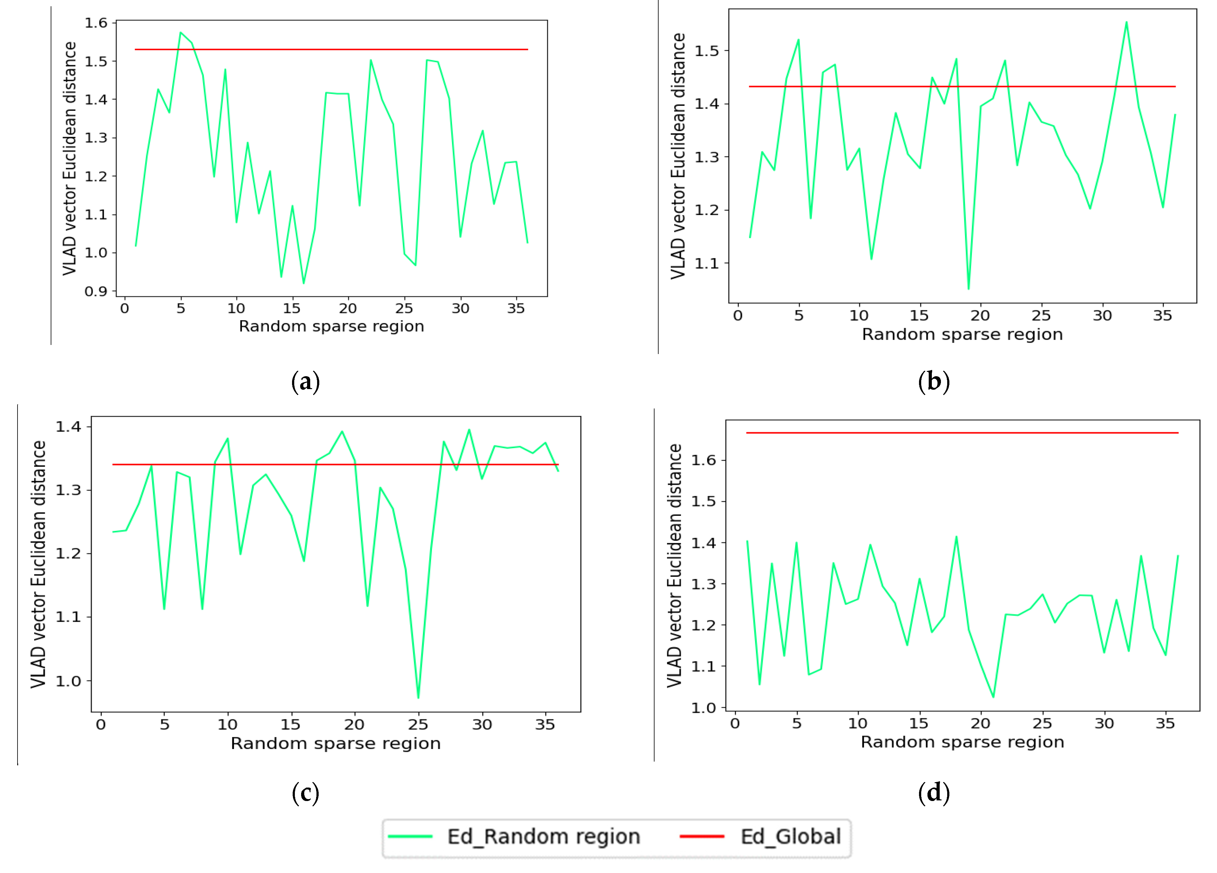
3.3. Detection of Feature-Sparse Regions and Measurement of Similarity

The SD-ME algorithm uses a feature-sparse region detector to detect feature-sparse regions in the UAV and satellite images, and then uses an adaptive feature thresholding algorithm to re-extract their features, thereby enhancing the matching process. Here, we validated the SD-ME algorithm on the four image pairs shown in Figure 4. The initial matches found using SuperGlue and SuperPoint for these images are shown in Figure 6.

Figure 6 shows that the SuperGlue + SuperPoint combination performed reasonably well on the UAV–satellite image pairs. However, very few matching points were found in the texture-sparse regions (e.g., vegetation, water bodies, and fields), which makes it difficult to utilize these results to globally and uniformly calibrate UAV images. The image feature maps of image pairs a–d have been visualized in Figure 7 to illustrate how globally consistent texture differentiation and feature detection thresholds affect feature extraction and descriptors in feature-sparse regions.

Figure 7 shows that variations in gradient are large in texturally dense regions (houses and roads) but small in texturally sparse regions (vegetation, water bodies, and farmland). Nonetheless, changes in gradient are still detectable even in texture-sparse regions. Due to the use of globally consistent texture differentiation and feature detection thresholds, the features of texture-sparse regions will be “masked” by those of texture-dense regions. As the former has very few matching points, the global distribution of matching points will become heterogeneous.

SD-ME was used to extract features from feature-sparse regions in the four UAV images shown in Figure 4, based on the initial matches found using SuperPoint and SuperGlue, with S = 256. The feature-sparse regions that were detected using the feature-sparse region detector were independently stored in a linked list. To create an intuitive view of the results, the feature-sparse regions were agglomerated, as shown in Figure 8.

As shown in Figure 8, the feature-spare region detector was able to acquire reliable feature-sparse regions. However, it is critical for the feature-sparse regions to have strict one-to-one correspondences for successful feature extraction and matching. Since different feature-sparse regions will have extremely low feature similarity, the validity of the results obtained by the feature-sparse region detector was tested by computing the feature similarity of the paired regions.

The local features in each region must be agglomerated to measure feature similarity. To this end, the Vector of Locally Aggregated Descriptors (VLAD) was used to aggregate the local descriptors of the feature-sparse regions [28]. The VLAD algorithm is a classic image search algorithm. In this algorithm, a codebook for a number of visual words is first trained using k-means clustering and each local descriptor is associated to its closest codebook centroid. The differences between all features and their centroids are accumulated to obtain d-dimensional vectors that each correspond to a visual word in the codebook, and concatenating these vectors then yields the VLAD vector of the image.

The UAV and satellite images tend to have low feature similarity due to ground object differences and nonlinear radiation distortions. Nonetheless, their feature similarities will still be globally consistent; in other words, the VLAD vector similarities of paired feature-sparse regions will be consistent with the VLAD vector similarity of the image pair as a whole [29]. In contrast, non-pairing feature-sparse regions will have a much lower VLAD vector similarity than the image pair. In this experiment, similarity was measured vis-à-vis the Euclidean distance of the VLAD vector. The longer the distance, the lower the similarity, and vice versa [30]. The Euclidean distance between vectors $V_1=\left(x_1,x_2,\dots ,x_d\right)$ and $V_2=\left(y_1,y_2,\dots ,y_d\right)$ is given by Equation (8):

$$Ed=\sqrt{{{\displaystyle \sum }}_{i=1}^d{\left(x_i-y_i\right)}^2}$$

(8)

The VLAD vector similarities of the paired feature-sparse regions acquired using the feature-sparse region detector were computed to confirm the one-to-one correspondence and local feature similarities of these paired regions. The computed feature similarities of the feature-sparse regions are shown in Figure 9.

In Figure 9, the horizontal axis represents the 36 randomly selected pairs of feature-sparse regions. The vertical axis shows the Euclidean distance between the VLAD vectors of the paired regions. Ed_a is the VLAD vector of the first image pair, and Ed_a_random is the VLAD vector of a randomly selected feature-sparse region from the first image pair. As shown in Figure 9, the feature-sparse regions usually have smaller VLAD vector Euclidean distances than that between the paired UAV and satellite images. This confirms that the feature-sparse regions extracted using the feature-sparse region detector have a strict one-to-one correspondence with their paired region.

3.4. Matching Experiment and Analysis

To test the performance of the SD-ME algorithm in the detection of feature-sparse regions and match augmentation, matching performance tests were performed on the SD-ME, SIFT, ContextDesc [31], and SuperGlue algorithms using the four image pairs shown in Figure 4. Several performance metrics were used to evaluate these algorithms. SIFT is a local feature descriptor that is affine-invariant and robust against interference. ContextDesc is a deep learning algorithm suitable for multimodal image matching and uses visual context from high-level image representation and geometric context from two-dimensional key point distribution to augment feature descriptors (such as DELF).

In this experiment, the number of correct matching points (P), accuracy of matching points (MA), and matching time (t) were used to compare the aforementioned matching algorithms. Correct matching points are defined as features whose positions in the to-be-matched and reference images are separated by a distance smaller than the threshold given by Equation (9). P is the number of matching points that satisfy this condition, and its value reflects the basic matching performance of the algorithm.

$$Correct\left(x\right):\sqrt{{\left(x_i-H{x}_{ i}^{\prime }\right)}^2+{\left(y_i-H{y}_{ i}^{\prime }\right)}^2} \le \epsilon$$

(9)

In this equation, H is the manually fitted affine transform of the two images, which is used in lieu of the real affine transform. If the affine-transformed feature point$\left(x_{ i}^{’},y_{ i}^{’}\right)$ is separated from$\left(x_i,y_i\right)$ by a distance smaller than ε (ε = 3 in this study), it is adjudged to be a correct matching point. Manual fitting was performed using a variety of matching algorithms followed by manual judgement to ascertain whether the match is correct. Areas not recognized by the matching algorithms were magnified for manual feature extraction. Consequently, 36 uniformly distributed matching points were selected for the fitting of the affine transform.

MA is the ratio of correct matching points to all matching points, which can reflect the successful matching performance of the algorithm.

The results of the three aforementioned algorithms and the SD-ME algorithm are shown in

Table 1. Comparison of matching test results.

Image Pair		1	2	3	4
P/correct matching points	SIFT	14	0	0	16
	ContextDesc	53	13	36	20
	SuperGlue	877	206	170	281
	SD-ME	1112	455	417	509
MA/%	SIFT	0.29	0	0	0.69
	ContextDesc	1.08	0.52	1.13	0.86
	SuperGlue	95.32	93.21	92.39	96.80
	SD-ME	93.21	70.76	72.15	72.61
t/s	SIFT	1.4	1.38	1.36	1.41
	ContextDesc	5.81	5.26	4.99	4.95
	SuperGlue	0.59	0.55	0.51	0.60
	SD-ME	1.28	1.21	1.12	1.12

.

Table 1 shows that the SIFT algorithm performed poorly, as it is not suitable for the matching of UAV and satellite images with nonlinear radiation distortions and large ground object differences. The ContextDesc algorithm found a reasonable number of matching points, but its accuracy (rate of correct matches) was poor, and its matching time was much greater than that of other matching algorithms. The SuperGlue algorithm performed reasonably well on these MSRSIs as it had a large number of matching points and had high accuracy. As the SD-ME algorithm is an augmentation of the SuperGlue algorithm, its matching time was slightly longer than that of SuperGlue. Nonetheless, it had the highest number of correct matching points. Furthermore, the matching points are uniformly distributed, and the matching results of the SD-ME algorithm are shown in Figure 10.

Figure 10 shows that the SD-ME algorithm is well-suited for the matching of UAV images to reference satellite images. The SD-ME algorithm succeeded in acquiring a large number of correct matching points by enhancing the initial matches found using SuperGlue. Compared to SuperGlue, SD-ME increased the number of correct matching points in each image pair by an average of 95.52%. Hence, the SD-ME algorithm has addressed the weakness of the SuperGlue algorithm in feature-sparse regions, as it was able to obtain an adequate number of reliable feature matching points in feature-sparse regions, which resulted in a uniform distribution of matching points. To test the uniformity of the SD-ME-enhanced results, the SD-ME algorithm was compared to the SuperGlue algorithm in terms of the uniformity of their matching point distribution.

The uniformity of distribution of the matching points was computed from their distributional uniformity in five different directions [32] by dividing the images in five directions into ten different regions, as shown in Figure 11.

Statistically speaking, if the matching point pairs are uniformly distributed in all five directions, the variance of the number of matching points in each direction should be small, and vice versa. The uniformity of the matching points is given by Equation (10), where the larger the value of U, the better the uniformity, and vice versa.

$$U=-\mathit{log}(\frac{{{\displaystyle \sum }}_{i=1}^{10}{(V_i-mean\left(V\right))}^2}{10})$$

(10)

In this equation, V is the regional statistical distribution vector, which is formed by combining the number of matching points in the 10 regions.

The steps for computing the distributional uniformity of the matching points are shown in Algorithm 2.

Algorithm 2. Computing Distributional Uniformity of the Matching Points

Step 1. Divide the image in 5 directions into 10 regions, as per Figure 11 Step 2. Compute the number of matching points in each region Step 3. Combine the number of matching points in the 10 regions to form the regional statistical distribution vector, V Step 4. Use Equation (10) to calculate the distributional uniformity of the matching points

The distributional uniformities of the matching points computed using the SD-ME and SuperGlue algorithms are shown in

Table 2. Distributional uniformity of SuperGlue and SD-ME matching points.

Image Pair	1	2	3	4
SuperGlue	−12.42215	−11.41827	−11.19921	−10.61661
SD-ME	−9.88986	−6.643	−7.005	−7.33263

.

Table 2 shows that in all four image pairs, the matching points of the SD-ME algorithm have higher distributional uniformity scores than the SuperGlue algorithm. Since uniformity was calculated as a logarithm that reflects on variance in five directions, the matching points of the SD-ME algorithm are significantly more uniform than those of the SuperGlue algorithm. This proves that the SD-ME algorithm successfully detected feature-sparse regions and augmented the matching process, which greatly improved the uniformity of the matching points.

4. Conclusion and Discussion

4.1. Conclusions

We proposed the SD-ME algorithm that augments SuperGlue with a feature-sparse region detector and adaptive feature thresholding, to address the difficulty of matching texture-sparse regions in satellite and UAV images. The SD-ME algorithm first detected feature-sparse regions for feature extraction, and then applied an adaptive threshold to the detected features. In this way, an adequate and uniform distribution of local features was obtained. Finally, the SuperGlue algorithm was used to produce reliable and robust matching results. Matching tests were performed on four difficult-to-match image pairs to test the efficacy of the SD-ME algorithm. The SIFT and deep learning-based ContextDesc performed poorly on these image pairs, but the SD-ME algorithm performed well on all four pairs. Compared to the SuperGlue algorithm, the SD-ME algorithm captured a considerably larger number of correct matching points, especially in feature-sparse regions. Therefore, the SD-ME algorithm successfully addressed the weaknesses of the SuperGlue algorithm in texture-sparse regions.

4.2. Discussion

In addition to augmenting SuperGlue, the other contribution of the SD-ME algorithm is that its feature-sparse region detector and adaptive feature thresholding algorithm is expected to be applied to most CNN-based feature matching algorithms, in other image matching applications. Although the feature-sparse region detector and matching enhancement algorithm will slightly increase the matching time, this will be compensated by a marked improvement in matching efficacy. Therefore, further research will focus on improving computational efficiency to improve the matching efficacy while minimizing the computer time.

References

1. Tu, H.; Zhu, Y.; Han, C. RI-LPOH: Rotation-invariant local phase orientation histogram for multi-modal image matching. Remote Sens. 2022, 14, 4228. [Google Scholar] [CrossRef]
2. Yan, L.; Fei, L.; Chen, C.; Ye, Z.; Zhu, R. A multi-view dense matching algorithm of high resolution aerial images based on graph network. Acta Geod. Cartogr. Sin. 2016, 45, 1171–1181. [Google Scholar] [CrossRef]
3. Zhang, Y.; Wan, Y.; Shi, W.; Zhang, Z.; Li, Y.; Ji, S.; Guo, H.; Li, L. Technical framework and preliminary practices of photogrammetric remote sensing intelligent processing of multi-source satellite images. Acta Geod. Cartogr. Sin. 2021, 50, 1068–1083. [Google Scholar]
4. Cui, S.; Xu, M.; Ma, A.; Zhong, Y. Modality-free feature detector and descriptor for multimodal remote sensing image registration. Remote Sens. 2020, 12, 2937. [Google Scholar] [CrossRef]
5. Lowe, G. Sift-the scale invariant feature transform. Int. J. 2004, 2, 2. [Google Scholar] [CrossRef]
6. Ke, Y.; Sukthankar, R. PCA-SIFT: A more distinctive representation for local image descriptors. In Proceedings of the 2004 IEEE Computer Society Conference on Computer Vision and Pattern Recognition, CVPR 2004, Washington, DC, USA, 27 June–2 July 2004. [Google Scholar]
7. Morel, J.M.; Yu, G. ASIFT: A new framework for fully affine invariant image comparison. SIAM J. Imaging Sci. 2009, 2, 438–469. [Google Scholar] [CrossRef] [Green Version]
8. Bay, H.; Ess, A.; Tuytelaars, T.; Van Gool, L. Speeded-up robust features (SURF). Comput. Vis. Image Underst. 2008, 110, 346–359. [Google Scholar] [CrossRef]
9. Rublee, E.; Rabaud, V.; Konolige, K.; Bradski, G. ORB: An efficient alternative to SIFT or SURF. In Proceedings of the 2011 International conference on computer vision, Barcelona, Spain, 6–13 November 2011; pp. 2564–2571. [Google Scholar] [CrossRef]
10. Yang, J.B.; Fan, D.Z.; Yang, X.B.; Ji, S.; Lei, R. Deep learning based on image matching method for oblique photogrammetry. J. Geo-Inf. Sci. 2021, 23, 1823–1837. [Google Scholar] [CrossRef]
11. Yao, Y.X.; Zhang, Y.J.; Wan, Y.; Liu, X.; Guo, H. Heterologous images matching considering anisotropic weighted moment and absolute phase orientation. Geomat. Inf. Sci. Wuhan Univ. 2021, 46, 1727–1736. [Google Scholar] [CrossRef]
12. Yu, Q.; Ni, D.; Jiang, Y.; Yan, Y.; An, J.; Sun, T. Universal SAR and optical image registration via a novel SIFT framework based on nonlinear diffusion and a polar spatial-frequency descriptor. ISPRS J. Photogramm. Remote Sens. 2021, 171, 1–17. [Google Scholar] [CrossRef]
13. LI, J.; Hu, Q.; AI, M. RIFT: Multi-modal image matching based on radiation-variation insensitive feature transform. IEEE Trans. Image Process. 2020, 29, 3296–3310. [Google Scholar] [CrossRef]
14. Yan, L.; Wang, Z.Q.; Ye, Z.Y. Multimodal image registration algorithm considering grayscale and gradient information. Acta Geod. Cartogr. Sin. 2018, 47, 71–81. [Google Scholar] [CrossRef]
15. Dusmanu, M.; Rocco, I.; Pajdla, T.; Pollefeys, M.; Sivic, J.; Torii, A.; Sattler, T. D2-net: A trainable CNN for joint description and detection of local features. In Proceedings of the IEEE/CVF Conference on Computer Vision and Pattern Recognition, Virtual Event, 15–20 June 2019; IEEE: New York, NY, USA. [Google Scholar] [CrossRef]
16. Efe, U.; Ince, K.G.; Alatan, A. Dfm: A performance baseline for deep feature matching. In Proceedings of the IEEE/CVF Conference on Computer Vision and Pattern Recognition, Virtual Event, 19–25 June 2019; IEEE: New York, NY, USA. [Google Scholar] [CrossRef]
17. Noh, H.; Araujo, A.; Sim, J.; Weyand, T.; Han, B. Large-scale image retrieval with attentive deep local features. In Proceedings of the IEEE International Conference on Computer Vision, Venice, Italy, 22–29 October 2017; IEEE: New York, NY, USA; pp. 3456–3465. [Google Scholar] [CrossRef]
18. Lan, C.Z.; Lu, W.J.; Yu, J.M.; Xu, Q. Deep learning algorithm for feature matching of cross modality remote sensing images. Acta Geod. Cartogr. Sin. 2021, 50, 189–202. [Google Scholar] [CrossRef]
19. DeTone, D.; Malisiewicz, T.; Rabinovich, A. Superpoint: Self-supervised interest point detection and description. In Proceedings of the IEEE Conference on Computer Vision and Pattern Recognition Workshops, Salt Lake City, UT, USA, 18–22 June 2018; IEEE: New York, NY, USA; pp. 224–236. [Google Scholar] [CrossRef]
20. Sarlin, P.E.; DeTone, D.; Malisiewicz, T.; Rabinovich, A. Superglue: Learning feature matching with graph neural networks. In Proceedings of the IEEE/CVF Conference on Computer Vision and Pattern Recognition, Online, 16–18 June 2020; IEEE: New York, NY, USA; pp. 4938–4947. [Google Scholar] [CrossRef]
21. Sun, J.; Shen, Z.; Wang, Y.; Bao, H.; Zhou, X. LoFTR: Detector-free local feature matching with transformers. In Proceedings of the IEEE/CVF Conference on Computer Vision and Pattern Recognition, Montreal, QC, Canada, 11–18 October 2021; pp. 8922–8931. [Google Scholar] [CrossRef]
22. Simonyan, K.; Zisserman, A. Very deep convolutional networks for large-scale image recognition. arXiv 2014. [Google Scholar] [CrossRef]
23. Shelhamer, E.; Long, J.; Darrell, T. Fully convolutional networks for semantic segmentation. IEEE Trans. Pattern Anal. Mach. Intell. 2016, 39, 640–651. [Google Scholar] [CrossRef] [PubMed]
24. Alkhatib, W.; Rensing, C.; Silberbauer, J. Multi-label text classification using semantic features and dimensionality reduction with autoencoders. In Proceedings of the International Conference on Language, Data and Knowledge, Nicosia, Cyprus, 27–29 September 2017; Springer: Cham, Germany, 2017; pp. 380–394. [Google Scholar] [CrossRef]
25. Shi, W.; Caballero, J.; Huszár, F.; Totz, J.; Aitken, A.P.; Bishop, R.; Rueckert, D.; Wang, Z. Real-time single image and video super-resolution using an efficient sub-pixel convolutional neural network. In Proceedings of the IEEE Conference on Computer Vision and Pattern Recognition, 2016, Las Vegas, NV, USA, 27–30 June 2016; pp. 1874–1883. [Google Scholar] [CrossRef] [Green Version]
26. Mao, W.D.; Wang, M.J.; Zhou, J.; Gong, M. Minglun Gong Semi-dense Stereo Matching using Dual CNNs. In Proceedings of the IEEE Winter Conference on Applications of Computer Vision, Waikoloa Village, HI, USA, 3–8 January 2019; pp. 1588–1597. [Google Scholar] [CrossRef] [Green Version]
27. Cuturi, M. Sinkhorn Distances: Lightspeed Computation of Optimal Transport. Adv. Neural Inf. Process. Syst. 2013, 26, 2292–2300. [Google Scholar] [CrossRef]
28. Jégou., H.; Douze., M.; Schmid., C.; Pérez, P. Aggregating local descriptors into a compact image representation. In Proceedings of the IEEE Computer Society Conference on Computer Vision and Pattern Recognition, San Francisco, CA, USA, 13–18 June 2010; pp. 3304–3311. [Google Scholar] [CrossRef] [Green Version]
29. Qin, J.Q.; Lan, C.Z.; Cui, Z.X.; Zhang, Y.X.; Wang, Y. A Reference Satellite Image Retrieval Method for Drone Absolute Positioning; Geomatics and Information Science of Wuhan University: Wuhan, China, 2020. [Google Scholar] [CrossRef]
30. Arandjelović, R.; Gronat, P.; Torii, A.; Pajdla, T.; Sivic, J. NetVLAD: CNN architecture for weakly supervised place recognition. In Proceedings of the IEEE Conference on Computer Vision and Pattern Recognition, Las Vegas, NV, USA, 27–30 June 2016; pp. 5297–5307. [Google Scholar] [CrossRef] [Green Version]
31. Luo, Z.X.; Shen, T.W.; Zhou, L.; Zhang, J.H.; Yao, Y.; Li, S.W.; Fang, T.; Quan, L. ContextDesc: Local descriptor augmentation with cross-modality context. In Proceedings of the IEEE/CVF Conference on Computer Vision and Pattern Recognition (CVPR), Long Beach, CA, USA, 18–24 June 2019; IEEE: New York, NY, USA; pp. 2527–2536. [Google Scholar] [CrossRef] [Green Version]
32. Zhu, H.F.; Zhao, C.H. An Evaluation Method for the uniformity of image feature point distribution. Daqing Norm. Univ. 2010, 30, 9–12. [Google Scholar] [CrossRef]
Figure 1. Flow chart of the SD-ME algorithm.
Remotesensing 14 06214 g001
Figure 2. Detection of feature-sparse regions: (a) initialize detector, (b) first partitioning, (c) K-th partitioning, and (d) stop partitioning.
Remotesensing 14 06214 g002
Figure 3. The adaptive thresholding algorithm.
Remotesensing 14 06214 g003
Figure 4. Experimental images: (a) image pair a, (b) image pair b, (c) image pair c, and (d) image pair d.
Remotesensing 14 06214 g004
Figure 5. Matching performance with different values of S: (a) number of matching points, (b) computer time of the matching process (matching time), and (c) number of matches per unit time.
Remotesensing 14 06214 g005
Figure 6. Initial matches found by SuperGlue: (a) image pair a, (b) image pair b, (c) image pair c, and (d) image pair d. Note: the yellow dots are the initial matches found by SuperGlue.
Remotesensing 14 06214 g006
Figure 7. Visualization of feature maps: (a) image pair a, (b) image pair b, (c) image pair c, and (d) image pair d.
Remotesensing 14 06214 g007
Figure 8. Results of the feature-sparse region detector: (a) image pair a, (b) image pair b, (c) image pair c, and (d) image pair d.
Remotesensing 14 06214 g008
Figure 9. Similarity of paired feature-sparse regions: (a) image pair a, (b) image pair b, (c) image pair c, and (d) image pair d.
Remotesensing 14 06214 g009
Figure 10. Matching results of the SD-ME algorithm: (a) image pair a, (b) image pair b, (c) image pair c, and (d) image pair d. Note: the yellow dots are the initial matches found by the SuperGlue algorithm, and green lines are the augmented results.
Remotesensing 14 06214 g010
Figure 11. Division of an image in five directions: (a) horizontal, (b) vertical, (c) 45°, (d) 135°, and (e) center and periphery.
Remotesensing 14 06214 g011