Abstract
Photon-counting LiDAR can obtain long-distance, high-precision target3D geographic information, but extracting high-precision signal photons from background noise photons is the key premise of photon-counting LiDAR data processing and application. This study proposes an adaptive noise filtering algorithm that adjusts parameters according to the background photon count rate and removes noise photons based on the local mean Euclidean distance. A simulated photon library that provides different background photon count rates and detection probabilities was constructed. It was then used to fit the distribution relationship between the background photon count rate and the average KNN (K-Nearest Neighbor) distance ( = 2–6) and to obtain the optimal denoising threshold under different background photon count rates. Finally, the proposed method was evaluated by comparing it with the modified density-based spatial clustering (mDBSCAN) and local distance-based statistical methods. The experimental results show that various methods are similar when the background noise rate is high. However, at most non-extreme background photon count rate levels, the F of this algorithm was maintained between 0.97–0.99, which is an improvement over other classical algorithms. The new strategy eliminated the artificial introduction of errors. Due to its low error rates, the proposed method can be widely applied in photon-counting LiDAR signal extraction under various conditions.
1. Introduction
Photon-counting LiDAR is one of the advanced technologies in the field of laser detection that emerged in the late 1990s [1]. Relying on the ability to detect extremely weak echo, the photon-counting technology can record response events with only a few photon signals, enabling it to have high repetition frequency and long-distance detection capabilities under micro-pulse conditions. The laser single pulse energy is reduced, increasing the laser repetition frequency and the point cloud density. It has been successfully applied to airborne mapping, 3D imaging [2,3], and satellite Earth Observation [4,5]. For instance, the Advanced Topographic Laser Altimeter System (ATLAS) and the photon-counting LiDAR laser altimetry carried by the Ice, Cloud, and Land Elevation Satellite-2 (ICESat-2), successfully launched by the United States on 15 September 2018 [6], has demonstrated great potential in bathymetry estimation, ice monitoring, and forest cover surveys [7,8,9,10]. The high-sensitivity sensor enables most of the returned photons to be detected, but due to the influence of atmospheric scattering and dark counting, a large number of noise photons are covered in the vicinity of the real signal photons. The noise photons are prominent during the day and are greatly affected by the background of the sun, which is a challenge for the application of data products in remote sensing. Therefore, to determine the properties of these photons and implement the separation accurately, some representative photon denoising strategies have been developed.
The most basic point cloud denoising algorithm is based on the distance correlation histogram of echo photon events of several adjacent laser pulses [11]. The along-track distance and elevation are equally divided into many bins of the same size. The properties of photons can then be determined by applying the law of large numbers and counting the probability of photon events within these bins. This approach assumes that noise is randomly distributed within each bin while the signal photons are clustered into several bins, so that the peaks of the histogram represent the approximate location of the signal. However, the changeable terrain may cause severe aliasing between the signal bin and the noise bin, which cannot show the expected performance in a complex situation.
Previous studies have proposed several denoising algorithms for photon-counting LiDAR data. The classical denoising algorithms can be classified into three categories: raster image processing-based, density-based spatial clustering of applications with noise (DBSCAN), and localized statistics-based algorithms.
(1) The raster-based image processing method [12] needs to interpolate the point cloud data into an image and then use the image processing method for denoising. There is, however, a loss of precision when interpolating to images, negating the data advantage of photon-counting LiDAR. (2) The density statistics approach alleviates the reliance on a persistent probability distribution of equally probable background photons within each bin. Density clustering algorithms can find photon clusters of arbitrary shapes in noisy data. The algorithm requires manual input of two parameters: eps (the radius of the neighborhood photon P) and MinPts (the minimum number of points within the given neighborhood) [13]. These input parameters could introduce errors and affect the accuracy of the algorithm. Moreover, the algorithm has limited accuracy in dealing with complex terrains. Zhang and Kerekes et al. [14] proposed modifying the search area from a circle to an ellipse and increasing the weight in the horizontal direction. Huang et al. [15] also proposed an automatic denoising algorithm for photon clouds based on particle swarm optimization. Hao et al. [16] extended the density-based spatial clustering algorithm to 3D point cloud, which can be performed in 3D cells, calculate the point cloud density in 3D space, and set a threshold for denoising. Herzfeld et al. [17] proposed using the radial basis function (RBF) to calculate the weighted density as an adaptive threshold for denoising. In general, the density-based spatial clustering algorithm can remove part of the noise, but it is not effective when dealing with uneven surfaces, such as steep slopes, and is very sensitive to input parameters. At the same time, the background photon count rate dynamically changing along the track is not considered, which reduces the accuracy of the algorithm. (3) The localized statistics-based algorithms mainly use a series of local statistical parameters, including point density, feature vector, and Euclidean distance to obtain the frequency distribution histogram and select the threshold to eliminate noise [7,10,18,19,20]. Xiao et al. [20] proposed a denoising algorithm based on the Bayesian decision theory, which deduced the probability distribution function of the KNN distance (the distance between the query point and its th nearest neighbor) and calculated the difference between the signal and the noise. The photonic point cloud denoising algorithm based on local statistical parameters has good denoising ability, but the denoising effect is subject to the selection of statistical parameter thresholds. This method can effectively remove noise, but the denoising accuracy is mainly affected by the value of the threshold and , and the threshold is also affected by the background photon count rate, laser foot point, slope, and other factors. Therefore, how to accurately quantify the threshold and value still needs further research.
In this study, a detailed analysis of the parameter design is carried out because of the complexity of the parameter definition, based on the KNN algorithm. With this framework, the influence of the selection range of in the KNN distance on the denoising results is quantitatively analyzed, and the threshold for different background photon levels is adaptively adjusted so that the algorithm can still be used under the condition of the dynamically changing high background photon count rate. The framework for the study consists of two steps: (1) Establish a complete numerical analysis model to quantitatively estimate the distance to KNN between signal photons and noise photons, and accurately reconstruct their histogram distribution functions. (2) Normalize the distance between adjacent footprints and fit a function of the critical threshold of the KNN distance and the background photon count rate. The algorithm threshold will adaptively update based on the above fitting function and background noise level, which largely avoids the well-known defect of manual parameter adjustment in generalized, local clustering methods. Furthermore, a complete simulation system was built to evaluate and verify the theoretical feasibility of this algorithm and the proposed framework from different perspectives. Finally, we applied this framework to homemade UAV (Unmanned Aerial Vehicle) LiDAR data and the ICESat-2 data under intense daytime background noise.
2. Theoretical Analysis and Numerical Simulation
2.1. KNN Based Denoising Principle
The denoising principle is shown in Figure 1. The Euclidean distance between the signal and the noise with their nearest neighbors is significantly different. The echo signal photons are confined within the pulse width, so the distance between the query point and neighboring points is less than the defined distance threshold. While the noise photons are randomly distributed in the 2D profile point cloud, the distance will be significantly larger than the distance threshold. Signal and noise can be classified clearly according to Euclidean distance differences. The denoising algorithm is a classification problem; it classifies the photon events we measure as signal or noise photons.
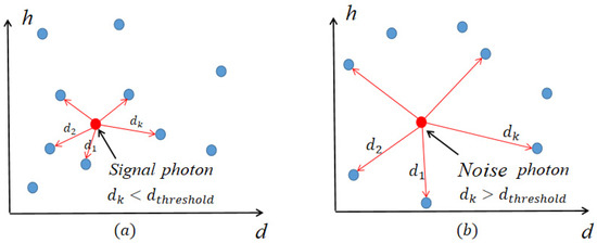
Figure 1.
Schematic diagram of KNN-based denoising. (a) Schematic diagram of the distribution of the signal photon and its nearest neighbors. (b) Schematic diagram of the distribution of the noise photon and its nearest neighbors.
The KNN algorithm classifies photon events based on the Euclidean distance. First, it needs to calculate the distance between each query point and its neighbors :
where represents the query point and represents the th closest point to the query point. As shown in Figure 1, when the distance from the th point is short, the query point is more likely to be a signal photon; otherwise, it is generally defined as noise. Therefore, the KNN algorithm needs to determine two core parameters: and the threshold of distance.
In addition, during intense solar background, the distribution of noise photon events is very dense, and the Euclidean distance of the noise will be relatively small, so the noise photon events can be misidentified as signals. Therefore, the threshold design must adaptively adjust to the noisy photon events.
In this work, two main parameters affect the KNN-based algorithm:
- (I)
- Determine kth: the query point and its kth nearest neighbors.
Determining the value of for photon events in profile is an essential part of the KNN filtering process. Excellent extraction performance needs to adopt an appropriate value, and a low value means increased random errors. Similarly, an excessively high value of causes distant and irrelevant samples to affect the results, weakening the centrality advantage of the clustering method.
- (II)
- Threshold: based on denoising.
The algorithm calculates the average distance between the photon and its nearest points as the criterion, so the threshold is the direct basis for distinguishing the signal from the noise. For signal photons, the signal photon will be confined to the width of the echo pulse and will be closer to other neighboring points on the two-dimensional profile point cloud. Considering this characteristic, the Euclidean distance between signal photons obtained by adjacent pulses is much lower than noise. Therefore, they have an optimal critical threshold, so the signals are distinguishable. Unfortunately, most of these methods rely on unintelligently adopting an empirical strategy or artificial selection based on histograms, introducing human error.
All in all, the value of and the threshold selection are related to the laser repetition frequency, the background photon count rate, and the moving speed of the light spot on the ground. Consequently, we first generated a labeled artificial photon database according to the characteristics of the photon Poisson distribution. The quantitative research of the simulated echo signal of KNN distance distribution is carried out.
2.2. Photon Events Generation
To evaluate this algorithm, this paper first designed a flow to generate a 2D profile, point cloud data of the echo “signal” of the LiDAR. The horizontal axis is the distance of the laser foot point along the track and the vertical axis is the height. The laser repetition frequency and the spot movement speed determine the horizontal distance between the adjacent laser pulse. Hence, the noise simulation only needs to consider two parameters: the distance between the centers of the adjacent pulses laser footprints and the background photon count rate.
In the photon-counting LiDAR system, the Poisson distribution can approximate the detection probability of the single-photon detector. For the signal with the average count rate , within τ time, the average number of photons is , and in this time range, the probability of detecting photons is as follows, which can derive from [21]:
Thus, the probability of no photons detected is:
The probability of detecting a photon is:
The process of generating a simulated signal is shown in Figure 2. First, the count rate of noise and signal photons should be determined. The background can be considered constant over short-time scales, so the background noise count rate is uniformly distributed along the time-of-flight. The flight time of the echo pulse is divided into multiple even bins and the width of each bin is estimated using the time resolution of the LiDAR. This study is based on the temporal resolution (64 ps) of the homemade UAV (Unmanned Aerial Vehicle) LiDAR. As the calculated probability is the probability that the number of photons in each bin is greater than or equal to one, the smaller the bin width setting, the greater the probability of a single photon in each bin. Hence, a small bin width is selected to ensure that the number of photons in each bin is less than or equal to 1. The detection probability was calculated from the photon background count rate based on Equation (3). The background photons obey the Poisson distribution and the simulated noise photons in the bin corresponding to a single laser pulse are generated based on the detection probability. Thus, the noise photons corresponding to each pulse are generated as shown in Figure 2b, where the abscissa is the pulse signal and the ordinate is the flight time.
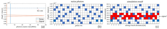
Figure 2.
Schematic diagram of simulation signal generation process. (a) Schematic diagram of signal and noise photon count rate as a function of flight altitude. (b) Schematic diagram of the noise photon corresponding to each pulse—the blue points are noise photons. (c) Simulation of the two-dimensional profile diagram, where the blue points are noise photons and the red points are signal photons.
Signal and noise are generated similarly, but the signal photon echo is confined in echo pulse width. After the single echo pulse is evenly divided into several bins along the flight time, the signal photon count rate is determined based on the detection probability of the echo signal. A random Poisson distribution can be generated to be the signal photon. At the same time, it should be noted that the signal has a certain broadening and the echo signal exhibits a Gaussian distribution.
Furthermore, convert the abscissa of the noise and the signal to distance along the track. The LiDAR system parameters determine the distance between the adjacent laser pulse foot points. The K-distance model will be changed due to the different distance between adjacent footprints. In order to obtain the suitable algorithm parameters for other various systems, the footprint distance of the simulation model is fixed. When applying this algorithm to the process point cloud collected by other systems, the distance between adjacent footprints should first be scaled proportionally. After comprehensively considering the parameters of the homemade UAV LiDAR and ICESat-2, the distance between laser pulses is defined as 0.1 m and the pulse width is 10 microseconds. After converting the ordinate to elevation through time-of-flight, the simulated 2D profile point cloud is obtained by combining the signal and noise.
The noise photon events are simulated by changing the background photon count rate and the distance between the center of adjacent footprints. Thereafter, the background noise with the same characteristics, but different background photon count rates collected by the single-photon LiDAR system, can be obtained by a two-dimensional Poisson distributed random number algorithm.
The signal and noise have the same horizontal and vertical grid width, while the echo beam and the transmit beam have the same Gaussian cross-section. Different detection probabilities are used to reverse the average signal photon number for different objects with different reflectivity. The echo signal model with a Gaussian distribution was simulated accordingly to study the denoising ability of the algorithm under different detection probabilities. The simulation results of signals with different detection probabilities are shown in Figure 3 and Figure 4.
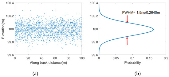
Figure 3.
Signal simulation results without noise (p = 0.25). (a) Two-dimensional scatter plot of signal simulation results. (b) When p = 0.25, the detection probability distribution of photons arriving at different altitudes, and its FWHM = 1.5 ns/0.2640 m.
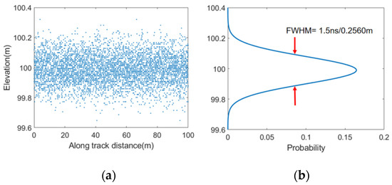
Figure 4.
Signal simulation results without noise (p = 0.55). (a) Two-dimensional scatter plot of signal simulation results. (b) When p = 0.55, the detection probability distribution of photons arriving at different altitudes, and its FWHM = 1.5 ns/0.2560 m.
Aimed at the background photon count rate, which is mostly in the range of 20 MHz, this study generates simulated background noises from 0.5 to 20 MHz at every 0.5 MHz. The signal detection probabilities range from 0.01 to 1 and generate 50 signal photons with different detection probabilities. The 2D profile point cloud of the simulated signal is shown in Figure 5:
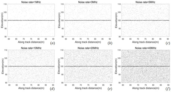
Figure 5.
Results from noise photon events and signal photon events (p = 0.55). (a) Background photon count rate is 1 MHz. (b) Background photon count rate is 3 MHz. (c) Background photon count rate is 5 MHz. (d) Background photon count rate is 10 MHz. (e) Background photon count rate is 20 MHz. (f) Background photon count rate is 40 MHz.
2.3. KNN Distribution of Noise Events
For this study, the simulation noise under the background photon count rate of 5 MHz is selected for quantitative research and description. From the mean value of ( = 2–6), the neighboring points of the Euclidean distance histogram distribution of the noise, shown in Figure 6, indicate a nonsymmetrical Gaussian distribution. On the left side of the peak, the signal increased rapidly with distance; in contrast, the right side of the peak decreased exponentially with distance. Therefore, it can be fitted by the product form of the exponential function and the power functions’ product forms. The probability density function of the distribution is:
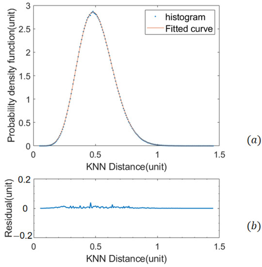
Figure 6.
Distribution model of noise (background photon counts rate = 5 MHz). (a) The neighboring points of the Euclidean distance histogram distribution of the noise (b) Residuals between the fitted results and the true results.
Hence, for a background photon count rate of 5 MHz, ; ; ; . The function fit is very close to the statistical results, which showed that the residual is less than 0.05, accounting for about 1.67% of the peak value.
Since different background photon count rates will lead to different distribution models of noise, the threshold value needs to be adaptively selected according to background conditions.
2.4. Optimization of k Parameter
In terms of value, the localized statistics-based algorithms calculate the distance and the average value of the distance between the query point and the neighboring points. The value is defined as 50, which is derived through empirical judgment, meaning quantitative studies have not been conducted [22,23,24]. Different values of directly affect how much neighborhood the algorithm operates in, which determines how many points the nearest neighbors around the photon will participate in the decision. This study quantitatively analyzed the selection of different values to determine the optimal range of .
The threshold was designated as 0.1%, and the average of points from i to j was chosen for calculating the F value under different combinations to analyze the effect of the algorithm quantitatively. Before conducting a quantitative study, three evaluation parameters need to be introduced for evaluating an algorithm’s denoising ability and precision: recall R, precision P, and F value are required to quantitatively describe the denoising ability of the algorithm [14]. The R represents the ratio of the number of correctly extracted effective photons to the total number of original photon signals. P represents the ratio of the number of correctly extracted effective photons to the total number of extracted photons. The F value represents the harmonic average of the recall rate and the precision rate. The larger the F number, the better the separation effect is. Among them, TP, FP, and FN represent the number of photon signals correctly identified, the number of noise photon point clouds that are wrongly classified into signal photon point clouds, and the number of photon signals that are not correctly identified, respectively.
Figure 7 shows the F-number distribution of the algorithm for different ( = i–j). As for the range of values, i and j continue to increase and distant irrelevant photons participate in the decision-making, consequently decreasing the algorithm’s precision. Finally, when = 2–6, the F-number of the algorithm is the highest and the denoising effect has the highest performance. The optimal k = 2–6 is the result at the background photon-counting rate of 5 MHz. If the LiDAR has a higher background photon-counting rate, a slightly larger k should be better.
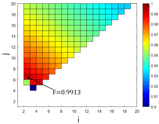
Figure 7.
Influence of different values on F (background photon counts rate = 5 MHz).
2.5. Threshold Model
It is necessary to count the cumulative probability distribution of the histogram distribution of the noise distribution since the threshold needs to reject most of the noise photons. In low background photon count rate conditions, the R of the signal is very high and does not change with minimal threshold changes, so the threshold setting is relatively strict to ensure the high accuracy of the algorithm. However, the signal’s recall rate and accuracy rate should be considered more comprehensively in the case of a higher background photon count rate. Therefore, when the background photon count rate and the threshold are fitted, two rejection regions are considered, respectively 99.9% and 90%, and the thresholds under different rejection regions are obtained.
The location of the threshold is affected by the distance between the background photon count rate and the laser foot point. Therefore, because the background photon count rate dynamically changes along the track, as does the distance between the adjacent laser foot points of different photon-counting LiDAR systems, the threshold should be adaptively calculated at the detection level to avoid the artificial introduction of errors. Due to the influence of solar radiation and surface reflection, the background photon count rate in the horizontal direction of the observed data is heterogeneous. If the change of the background photon count rate is not considered, and the threshold is directly defined as a constant, the noise will be misjudged as photons where the background photon count rate is high, and the recall rate of the signal will be affected where the background noise count rate is low. Therefore, in processing the actual data, it is necessary to calculate the background photon count rate in the grid corresponding to each beam for the dynamically changing background radiation intensity and adaptively obtain the threshold value according to the distance between adjacent lasers. Based on the simulated noise signal, the function between the threshold and the background photon count rate is studied after the normalization of the LiDAR footstep interval (0.01 m was selected for this study due to the characteristics of different LiDAR systems). The threshold value can be calculated by bringing the background photon count rate into the fitting function for the dynamically changing background photon count rate in processing real signals. Hence, the fitting relationship between the background photon count rate and the threshold under different rejection regions is obtained from the two rejection regions (99.9% and 90%) as shown in Figure 8. The fitting result is shown in Figure 9:
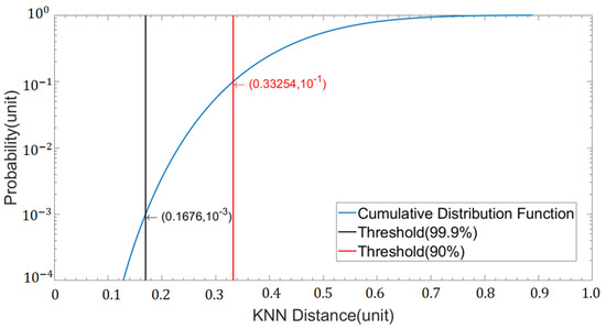
Figure 8.
The cumulative probability distribution to determine the threshold position (background photon counts rate = 5 MHz).
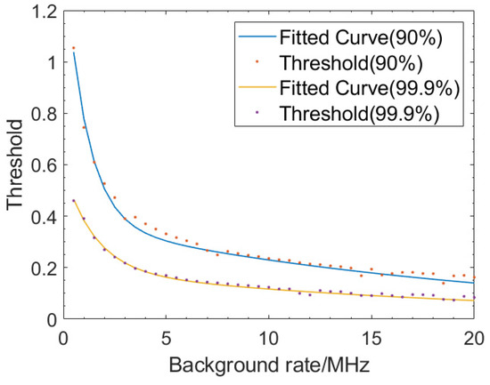
Figure 9.
Model rejecting 99.9% and 90% probability distribution location.
Use the power function to fit the background photon count rate and the threshold. The fitting function adopts:
where is the background photon count rate. When is the threshold, in case of rejection, regions equal 99.9%,.
In case of rejection, regions equal 90%, .
As the count rate changes, a scale factor () is defined as a smooth step function related to the background photon count rate as shown in Figure 10, which can tune different rejection domains based on their background photon count rate. For strong background cases, we selected a relatively loose threshold at the 90% probability distribution point to reduce signal loss. As a comparison, the threshold at 99.9% probability distribution point is used under the weak background conditions. A scale factor q that varies with the background photon-counting rate is used for the transition areas between strong and weak backgrounds.
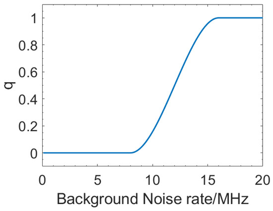
Figure 10.
Smooth step function related to the background photon count rate.
With an increasing background photon count rate, the contradiction between the recall rate and the accuracy rate is constantly balanced. For instance, at the background photon count rate of 8 to 16 MHz, the threshold selection is iteratively relaxed as the background photon count rate increases. The final threshold selection formula:
where is the scale factor that is changed with the background. is the threshold in case of rejection regions equal to 99.9%, is the threshold in case of rejection regions equal to 90%.
When processing real signals, after normalizing the step size, the background photon count rate is brought in according to the fitting function formula for the adaptive selection of the threshold.
When = 2–6, the histogram distribution model of noise and signal is shown in Figure 11, which has various distributions, so the threshold can be denoised accordingly.
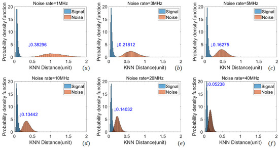
Figure 11.
Distribution of signal and noise histograms (p = 0.55). (a) Background photon count rate is 1 MHz. (b) Background photon count rate is 3 MHz. (c) Background photon count rate is 5 MHz. (d) Background photon count rate is 10 MHz. (e) Background photon count rate is 20 MHz. (f) Background photon count rate is 40 MHz.
2.6. Optimal Parameter of the Denoising Algorithm
The following processes were formulated to calculate the parameters of the denoising algorithm in different LiDARs, since they have different repetition frequencies and footprint intervals. The main flow of the framework is as follows:
- Generation of a 2D profile point cloud: the abscissa is the distance along the track and the ordinate is the height;
- Normalizing the distance between the laser feet (set to 0.01 m in this study);
- Construction of a K-D tree to improve search efficiency;
- Calculation of the average distance between the photon and its nearest neighbor k photons based on Equation (1);
- Calculation of the background photon count rate corresponding to each laser pulse. The background photon count rate that varies along the track is brought into the fitting Equation (9) to calculate the corresponding threshold;
- Determine the relationship between the average value of the distances of the nearest k points corresponding to each point and the threshold value. If it is less than the threshold value, it is determined as a valid signal photon. Otherwise, it is a noise photon.
3. Results
Three statistical evaluation indicators were selected to verify the denoising ability of the algorithm: recall R, precision P, and F value. mDBSCAN parameter selection was consistent with the literature [14], and the threshold was set to four times the average point density. The KNN algorithm [22] selects the classic = 50, and the threshold is selected as the distance of twice the standard deviation of the noise distribution histogram.
The background noise count rate is from 1 to 15 MHz, and the detection probability is 0.15, 0.25, and 0.55 for simulated noise and signal to test the denoising ability of the three algorithms under different conditions, respectively.
According to Table 1, mDBSCAN has a passable denoising ability under a high background photon count rate. The original KNN algorithm will be affected by the increase of the background photon count rate and the recall and precision, which will decrease with the increase of the background photon count rate. As the background photon count rate calculates the threshold, the precision of our algorithm is less restricted by the background photon count rate. It can still maintain high precision and ensure the recall of the signal at a higher background photon count rate. Compared with available algorithms, the F can be improved. In a high-noise environment with a background photon count rate of 13 MHz and a detection probability of 0.55, the recall of the traditional density-based clustering algorithm can reach 1.0000. However, the precision can only reach 0.8294 due to the high background noise. Under the same conditions, the precision of the KNN after the parameter optimization algorithm is significantly improved and can reach 0.9532. At the same time, this algorithm has great advantages for the background photon count rate that changes dynamically along the track.

Table 1.
Three statistical indicators of simulated data with three noise rates based on the modified DBSCAN algorithm, the original KNN algorithm, and the KNN after parameter optimization.
4. Discussion
4.1. Optimal Parameter of the Denoising Algorithm
In this study, a photon-counting LiDAR system was built, and its structure is shown in Figure 12.
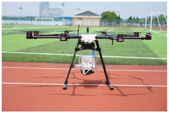
Figure 12.
Instrument illustration.
The laser radar transmitting system emits a linearly polarized laser with a wavelength of 523 nm, single pulse energy of 200 nJ, a pulse width of 1 ns, and a laser repetition frequency of up to 500 kHz. The LiDAR uses a mirror to perform conical scanning. The angle between the motor’s rotation axis and the incident laser is 45°; the normal direction of the mirror is 7.5° to the motor’s rotation axis, achieving a conical scan with a maximum width of ±15°. The effective diameter of the receiving telescope is 10 mm and the receiving field of view is 2 mrad. The detector has a quantum efficiency of 18% at 532 nm, a TDC (Time-to-Digital Converter) time resolution of 64 ps, and a corresponding distance resolution of 0.0096 m. Furthermore, a narrow-band filter with a bandwidth of 0.5 nm is set in the LiDAR to suppress the influence of solar background radiation. During daytime observation, an additional 10% transmittance-neutral filter is added to the receiving system to reduce the influence of intense solar background radiation. The final system weighs no more than 6 kg and consumes no more than 50 W.
The orbit height of ICESat-2 [25] is about 500 km, the inclination angle is 92°, the repetition period is 91 days, and each period has 1387 orbits. The ATLAS system is equipped with two lasers, which emit 532 nm laser pulses at a repetition rate of 10 kHz with a pulse width of 1.5 ns, and obtains overlapping spots with an interval of about 0.7 m along the track and a diameter of 17 m. The main parameters of the homemade Lidar and ICESat-2 are shown in Table 2.
Table 2.
Main specifications of the system.
In this experiment, the scanning mode was selected as the conical scanning mode. Unlike the linear scan structure, the laser beam of the conical scan system maintains an approximately fixed angle of incidence. The conical scanning structure installs a mirror in front of the laser, adjusting the incident angle of the laser beam between the normal line of the mirror and the horizontal line of the laser, and the angle between the mirror and the rotation axis, so that the laser beam is at a certain angle. The laser pinpoint will form an elliptical trajectory when the mirror rotates at high speed. The angle of the mirror can be counted by fixing the encoder on the drive motor shaft. The distance between the corresponding adjacent laser foot points is 0.0034 m.
4.2. Denoising Results for Photon-Counting LiDAR Data
The tidal flat near Fisherman’s Wharf in the Fengxian District, Shanghai, was selected for the homemade LiDAR experiment. The location has prominent geomorphological features, so it was suitable for verifying the detection performance of the airborne LiDAR system. The background photon count rate is mainly between 0.1 and 1.5 MHz. The raw data were projected to a two-dimensional elevation profile, where the horizontal axis is the distance along the laser track and the vertical axis is the height.
In ICESat-2, the data [26] were selected with high background photon count rate at 15.26.44 pm in the Sahara Desert near the equator. The average background photon count rate is as high as 2.84 MHz, and the maximum background photon count rate can reach 18.4435 MHz. The denoising ability under the condition was evaluated.
When denoising the instrument data, the background photon count rate corresponding to each laser pulse is calculated and then brought into the fitting function to obtain the threshold value. After that, the distance to the KNN corresponding to each photon is subtracted from the threshold value. If the result is greater than zero, it is reserved for the signal photon; otherwise, the noise needs to be filtered out.
Figure 13 shows the processing result of the homemade LiDAR, while Figure 14 shows the processing result of the ICESat-2. (a) The original 2D cross-sectional point cloud image; (b) The background photon count rate along the track direction. It can be seen that the background photon count rate is distributed unevenly along the track direction, from 0.05 to 0.45 MHz; (c) The two-dimensional image of the threshold minus the query point difference. The part greater than zero is reserved for the signal. The range between signal and noise is quite different. (d) The image after denoising. A good denoising effect was achieved.
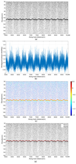
Figure 13.
(a) Original homemade LiDAR data. (b) Background photon counts rate. (c) Threshold minus the KNN distance of query points. (d) Denoised results.
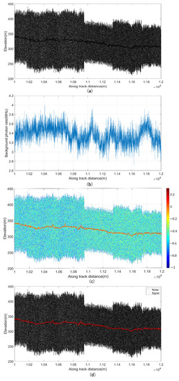
Figure 14.
(a) Original ICESat-2 data. (b) Background photon counts rate. (c) Threshold minus the KNN distance of query points. (d) Denoised results.
To evaluate the accuracy of the denoising algorithm, a dataset including both signal and noise photons was generated at the Poisson distribution model of the photons. The benefit of this approach is that the label of each simulated photon event is unambiguous. Of course, the simulated photon events does not consider the influence from the non-ideal properties of the detector and acquisition system, such as the dead time and after pulse effects. When the background photon-counting rate is extremely strong, the simulated data will deviate with the actual situations.
5. Conclusions
In this study, a 2D profile point cloud data of the LiDAR’s echo “signal” was generated using simulations based on probability distribution functions. The database created from this simulation was used to study the selection method of the two parameters that influence different background photon count rates on the threshold after normalizing the distance between different laser foot points. By selecting the position that automatically adjusts based on the background photon count rate, to reject 90% to 99.9% of noise as threshold, the relational expressions are fitted, and the denoising ability of the algorithm is verified in the simulation data. The observation data with a high background photon count rate dynamically changing along the track, counted the background photon count rate at each laser pulse. The optimal threshold was also adaptively calculated, thereby avoiding the artificial introduction of errors while balancing the R and P of the algorithm. Under the condition of the background photon count rate that changes drastically along the track, the algorithm has a gratifying denoising performance. Future work should be dedicated to applying our algorithm to more scenarios and evaluating the algorithm comprehensively.
Author Contributions
Conceptualization, R.M., W.K., T.C., R.S. and G.H.; Writing—original draft, R.M.; Writing—review & editing, W.K.; Project administration, R.S. and G.H. All authors have read and agreed to the published version of the manuscript.
Funding
This research was funded in part by the Shanghai Municipal Science and Technology Major Project No. 2019SHZDZX01, Innovation Program for Quantum Science and Technology of Ministry of Science and Technology of China No. 2021ZD0301400, National Natural Science Foundation of China No. 61875219, Youth Innovation Promotion Association, Chinese Academy of Sciences, Shanghai Rising-Star Program No. 22QA1410500, and Innovation Foundation of Shanghai Institute of Technical Physics, Chinese Academy of Sciences No. CX-308.
Conflicts of Interest
The authors declare no conflict of interest.
References
- Degnan, J.J.; Mcgarry, J.F.; Zagwodzki, T.W.; Dabney, P.W.; Chu, A. Design and Performance of a 3D Imaging Photon-Counting Microlaser Altimeter Operating From Aircraft Cruise Altitudes Under Day or Night Conditions. In Laser Radar: Ranging and Atmospheric Lidar Techniques III; SPIE: Bellingham, WA, USA, 2002; Volume 4546, pp. 1–10. [Google Scholar]
- Li, Z.P.; Ye, J.T.; Huang, X.; Jiang, P.Y.; Cao, Y.; Hong, Y.; Yu, C.; Zhang, J.; Zhang, Q.; Peng, C.Z.; et al. Single-Photon Imaging Over 200 km. Optica 2021, 8, 344–349. [Google Scholar] [CrossRef]
- Jiang, P.Y.; Li, Z.P.; Xu, F.H. Compact Long-Range Single-Photon Imager with Dynamic Imaging Capability. Opt. Lett. 2021, 46, 1181–1184. [Google Scholar] [CrossRef] [PubMed]
- Dabney, P.; Harding, D.; Abshire, J.; Huss, T.; Zheng, Y. The Slope Imaging Multi-polarization Photon-Counting Lidar: Development and Performance Results. In Proceedings of the 2010 IEEE International Geoscience and Remote Sensing Symposium, Honolulu, HI, USA, 25–30 July 2010; IEEE: Piscataway, NJ, USA, 2010; pp. 653–656. [Google Scholar]
- Degnan, J.; Wells, D.; Machan, R.; Leventhal, E. Second generation airborne 3D imaging lidars based on photon counting. In Advanced Photon Counting Techniques II; Becker, W., Ed.; SPIE: Bellingham, WA, USA, 2007; Volume 6771, p. N7710. [Google Scholar]
- Markus, T.; Neumann, T.; Martino, A.; Abdalati, W.; Brunt, K.; Csatho, B.; Farrell, S.; Fricker, H.; Gardner, A.; Harding, D.; et al. The Ice, Cloud, and Land Elevation Satellite-2 (ICESat-2): Science Requirements, Concept, and Implementation. Remote Sens. Environ. 2017, 190, 260–273. [Google Scholar] [CrossRef]
- Nie, S.; Wang, C.; Xi, X.; Luo, S.; Li, G.; Tian, J.; Wang, H. Estimating the Vegetation Canopy Height Using Micro-pulse Photon-Counting LiDAR Data. Opt. Express 2018, 26, A520–A540. [Google Scholar] [CrossRef] [PubMed]
- Albright, A.; Glennie, C. Nearshore Bathymetry from Fusion of Sentinel-2 and ICESat-2 Observations. IEEE Geosci. Remote Sens. Lett. 2020, 99, 1–5. [Google Scholar] [CrossRef]
- Chen, Y.; Le, Y.; Zhang, D.; Wang, Y.; Qiu, Z.; Wang, L. A Photon-Counting LiDAR Bathymetric Method Based on Adaptive Variable Ellipse Filtering. Remote Sens. Environ. 2021, 256, 112326. [Google Scholar] [CrossRef]
- Zhu, X.; Nie, S.; Wang, C.; Xi, X.; Hu, Z. A Ground Elevation and Vegetation Height Retrieval Algorithm Using Micro-Pulse Photon-Counting Lidar Data. Remote Sens. 2018, 10, 1962. [Google Scholar] [CrossRef]
- Brunt, K.M.; Neumann, T.A.; Walsh, K.M.; Markus, T. Determination of Local Slope on the Greenland Ice Sheet Using a Multibeam Photon-Counting Lidar in Preparation for the ICESat-2 Mission. IEEE Geosci. Remote Sens. Lett. 2013, 11, 935–939. [Google Scholar] [CrossRef]
- Magruder, L.A.; Wharton, M.; Stout, K.D.; Neuenschwander, A.L. Noise Filtering Techniques for Photon-Counting Ladar Data. In Laser Radar Technology and Applications XVII; SPIE: Bellingham, WA, USA, 2012; Volume 8379, p. 24. [Google Scholar]
- Ester, M.; Kriegel, H.P.; Sander, J.; Xu, X. A Density-Based Algorithm for Discovering Clusters in Large Spatial Databases with Noise; AAAI Press: Palo Alto, CA, USA, 1996. [Google Scholar]
- Zhang, J.; Kerekes, J. An Adaptive Density-Based Model for Extracting Surface Returns From Photon-Counting Laser Altimeter Data. IEEE Geosci. Remote Sens. Lett. 2014, 12, 726–730. [Google Scholar] [CrossRef]
- Huang, J.; Xing, Y.; You, H.; Qin, L.; Tian, J.; Ma, J. Particle Swarm Optimization-Based Noise Filtering Algorithm for Photon Cloud Data in Forest Area. Remote Sens. 2019, 11, 980. [Google Scholar] [CrossRef]
- Hao, T.; Swatantran, A.; Barrett, T.; Decola, P.; Dubayah, R. Voxel-Based Spatial Filtering Method for Canopy Height Retrieval from Airborne Single-Photon Lidar. Remote Sens. 2016, 8, 771. [Google Scholar] [CrossRef]
- Herzfeld, U.C.; Trantow, T.M.; Harding, D.; Dabney, P.W. Surface-Height Determination of Crevassed Glaciers-Mathematical Principles of an Autoadaptive Density-Dimension Algorithm and Validation Using ICESat-2 Simulator (SIMPL) Data. IEEE Trans. Geosci. Remote Sens. 2017, 55, 1874–1896. [Google Scholar] [CrossRef]
- Gwenzi, D.; Lefsky, M.A.; Suchdeo, V.P.; Harding, D. Prospects of the ICESat-2 laser altimetry mis-sion for savanna ecosystem structural studies based on airborne simulation data. ISPRS J. Photogramm. Remote Sens. 2016, 118, 68–82. [Google Scholar] [CrossRef]
- Herzfeld, U.C.; Mcdonald, B.W.; Wallin, B.F.; Neumann, T.A.; Markus, T.; Brenner, A.; Field, C. Algorithm for Detection of Ground and Canopy Cover in Micropulse Photon-Counting Lidar Altimeter Data in Preparation for the ICESat-2 Mission. IEEE Trans. Geosci. Remote Sens. 2014, 52, 2109–2125. [Google Scholar] [CrossRef]
- Wang, X.; Pan, Z.; Glennie, C. A Novel Noise Filtering Model for Photon-Counting Laser Altimeter Data. IEEE Geosci. Remote Sens. Lett. 2016, 13, 947–951. [Google Scholar] [CrossRef]
- He, W.; Sima, B.; Chen, Y.; Dai, H.; Chen, Q.; Gu, G. A Correction Method for Range Walk Error in Photon Counting 3D Imaging LIDAR. Opt. Commun. 2013, 308, 211–217. [Google Scholar] [CrossRef]
- Shaobo, X.; Cheng, W. XiXiaoHuan; LuoShe Weeks; Zeng Hongcheng, ICESat-2 Airborne Test Point Cloud Filtering and Vegetation Height Inversion. J. Remote Sens. 2014, 18, 1199–1207. [Google Scholar]
- Yiteng, X.; Guoyuan, L.; Chunxia, Q.; Yucai, X. Single Photon Laser Data Processing Technique Based on Terrain Correlation and Least Squares Curve Fitting. Infrared Laser Eng. 2019, 48, 148–157. [Google Scholar] [CrossRef]
- Syed, N.; Zhang, Y.; Tong, X.; Weiming, Y.; Peng, D. Denoising and Filtering Algorithm for single-photon LiDAR data. Navig. Control. 2020, 19, 67–76. [Google Scholar]
- Martino, A.J.; Neumann, T.A.; Kurtz, N.T.; Mclennan, D. ICESat-2 Mission Overview and Early Performance. Sens. Syst. NextGener. Satell. 2019, XXIII, 11151. [Google Scholar]
- Neumann, T.A.; Brenner, A.; Hancock, D.; Robbins, J.; Saba, J.; Harbeck, K.; Gibbons, A.; Lee, J.; Luthcke, S.B.; Rebold, T. ATLAS/ICESat-2 L2A Global Geolocated Photon Data, Version 5. [Indicate Subset Used]; NASA National Snow and Ice Data Center Distributed Active Archive Center: Boulder, CO, USA, 2021. [Google Scholar] [CrossRef]


Publisher’s Note: MDPI stays neutral with regard to jurisdictional claims in published maps and institutional affiliations. |
© 2022 by the authors. Licensee MDPI, Basel, Switzerland. This article is an open access article distributed under the terms and conditions of the Creative Commons Attribution (CC BY) license (https://creativecommons.org/licenses/by/4.0/).