Abstract
Floating-algae detection plays an important role in marine-pollution monitoring. The surveillance cameras on ships and shores provide a powerful way of monitoring floating macroalgae. However, the previous methods cannot effectively solve the challenging problem of detecting Ulva prolifera and Sargassum, due to many factors, such as strong interference with the marine environment and the drastic change of scale. Recently, the instance-segmentation methods based on deep learning have been successfully applied to many image-recognition tasks. In this paper, a novel instance-segmentation network named AlgaeFiner is proposed for high-quality floating-algae detection using RGB images from surveillance cameras. For improving the robustness of the model in complex ocean scenes, the CA-ResNet is firstly proposed by integrating coordinate attention into the ResNet structure to model both the channel- and position-dependencies. Meanwhile, the Ms-BiFPN is proposed by embedding the multi-scale module into the architecture of BiFPN to strengthen the ability of feature fusion at different levels. To improve the quality of floating-algae segmentation, the Mask Transfiner network is introduced into the AlgaeFiner to obtain the high-quality segmentation results. Experimental results demonstrate that the AlgaeFiner can achieve better performance on floating-algae segmentation than other state-of-the-art instance-segmentation methods, and has high application-value in the field of floating-macroalgae monitoring.
1. Introduction
The large-scale outbreaks of floating algae have become a worldwide ecological issue of the marine environment, recently. The wild breeding of floating algae, blocking the sunlight on the sea surface and the competition for nutrition with other ocean life, will affect the marine ecological structure. The rotting of a large number of seaweeds will cause severe pollution to the quality of the sea water, stacked along the coasts to destroy the natural environment of beaches [1]. Therefore, the disaster events involving floating macroalgae are harmful for the protection and development of marine resources, and have a significant impact on the economic industries such as aquaculture, fishery, maritime transportation and coastal tourism [2,3,4].
In recent years, the frequent outbreak of green tide and gold tide in the East China Sea is caused by two categories of floating algae—Ulva prolifera and Sargassum, which has the characteristics of short, explosive cycle and a large influence area [5,6,7]. Therefore, it is necessary to conduct real-time monitoring and early warning for floating algae. Furthermore, the accurate extracting and distinguishing of the floating algae could provide a reliable basis for the analysis, prevention, and comprehensive governance of disasters, to reduce economic costs and environmental disasters. Therefore, a variety of ways, such as remote-sensing satellite [8,9,10,11,12,13,14,15,16], synthetic-aperture radar (SAR) [17,18,19], unmanned aerial vehicles (UAV) [20,21,22,23,24], and the surveillance cameras on ships and shores [25,26,27], are applied to monitor floating algae.
In the past decades, a lot of floating-algae detection methods based on traditional image-processing algorithms have been researched. These methods, using threshold segmentation and image transformation, have the advantages of effective feature-extraction and low computing cost. Pan et al., proposed a two-step method to reduce the computational complexity of N-FINDR, based on spectral unmixing, and this model could estimate the green-algae area efficiently from the Geostationary Ocean Color Imager (GOCI) [28]. Wang et al., quantified the area coverage of Sargassum from Moderate Resolution Image Spectroradiometer (MODIS)-data in the western central Atlantic, based on the alternative floating algae index (AFAI) to detect the red-edge reflectance of floating algae [29]. Wang et al., introduced a trainable, nonlinear reaction– diffusion denoising framework to handle non-algae influence, and used the Floating Algae Index (FAI) to detect Sargassum from MSI images [30]. Ody et al., introduced the standard to describe various sizes of Sargassum, and compared the ability to detect Sargassum between in situ and remote-sensing observations (MODIS, VIIRS, OLCI and MSI) in the northern Tropical Atlantic [31]. Shen et al., proposed the new index factors based on the polarimetric characteristics of green tides in both the amplitude- and phase-domain, to detect green-macroalgae blooms from quad-pol RADARSAT-2 SAR images [32]. Ma et al., monitored the spatiotemporal trend of Ulva prolifera effectively, based on SAR and MODIS data in the Yellow Sea in 2021 [33]. Using the RGB cameras on ship-borne UAVs, Jiang et al., proposed a new floating algae index, calculating the difference in green reflectance from the baseline for red and blue bands, to extract green tide in the Yellow Sea, effectively [34]. Xu et al., introduced the normalized green–red difference index to detect the initial biomass of green tide accurately, from UAV and Sentinel-2A images [35].
The traditional methods for floating-algae segmentation based on image processing require a complex process of artificial-feature design, and cannot achieve the segmentation accurately under different weather conditions (such as sunny, cloudy or windy). With the great progress of deep learning recently, convolutional neural networks (CNNs), generative adversarial network (GAN) and transformer have been successfully applied in the fields of image segmentation [36] and object detection [37], as they have the advantages of extracting useful features automatically. Therefore, extensive research has been conducted on floating-algae detection using deep learning methods in recent years [38,39,40,41,42,43]. From the UAV hyperspectral imagery, Hong et al., introduced four different CNN frameworks (ResNet-18, ResNet-101, GoogLeNet, and Inception v3) to estimate the vertical distributions of the harmful algae, and gradient-weighted class-activation mapping was used to adopt the representative features [44]. Wang et al., proposed a green-tide detection framework based on a binary CNN-model and Superpixels extracted via energy-driven sampling (SEEDS) for high-resolution UAV images [45]. To monitor the distribution of Sargassum along the French Caribbean Sea, Valentini et al., adopted MobileNet-V2 architecture on the super-pixel regions extracted from the images captured by smartphone cameras [26]. A Sargassum-detection method was introduced, based on CNN and RNN from MODIS imagery collected along the Mexican Caribbean coastline [46]. To overcome the lower detection-limit of different sensors and the complex environment, Wang et al., introduced the VGGUnet network to extract Sargassum macroalgae, based on the high-resolution satellite images from multi-sensors such as MSI, OLI, WV and DOVE [47]. Cui et al., combined a semantic-segmentation network based on U-Net with super-resolution reconstruction to extract green tides accurately from low-resolution MODIS images, pre-trained from high-resolution GF1-WFV data [48]. Gao et al., introduced the U-Net method to design a green-algae detection framework from both MODIS and SAR data in the Yellow Sea [49]. Jin et al., proposed a GAN with a squeeze-and-excitation attention mechanism to detect green tide at different scales automatically from MODIS images in the Yellow Sea [50]. Arellano-Verdejo et al., introduced the Pix2Pix GAN semantic-segmentation architecture to monitor the Sargassum-coverage map from the photographs acquired by mobile devices along the beaches [27]. Song et al., proposed a cyanobacteria-detection model based on the transformer network, to extract the boundary of cyanobacterial blooms accurately in complex environments from UAV-multispectral images [51].
The object-detection methods can locate and classify objects in images, and do not concern the classification of each pixel. The faster R-CNN network, a classic model in object-detection methods, has achieved good results in the fields of high-precision, multi-scale and small-target detection [52]. The YOLOv7 is a current state-of-the-art network which surpasses a lot of known object-detectors in both speed and accuracy [53]. Nevertheless, these object-detection methods cannot obtain the accurate boundary of each object. The semantic-segmentation methods can effectively classify each pixel according to category, and obtain the accurate mask-boundary of each object. A new high-quality building-extraction method named the sparse-token transformer (STT) is proposed, to represent the building as a set of ‘sparse’-feature vectors in their feature space by introducing the ‘sparse-token sampler’, which can reduce computational complexity in the transformer [54]. A simple segmentation-method is proposed, even if only a few training images are provided, and can serve as an instrument for semantic segmentation, especially in the setup when labeled data is scarce [55]. However, the semantic-segmentation methods still have shortcomings in dealing with objects in the same category, because these methods only capture the target of different categories and cannot distinguish the individual algae in the same category. The instance-segmentation method can integrate object detection and semantic segmentation into a unified architecture, which can simultaneously detect and segment the individual object in the same category [56]. Therefore, it is meaningful to detect the floating algae based on the instance-segmentation algorithms.
As a pioneering work of the instance-segmentation method, the Mask R-CNN [57] has achieved great success in the field of image recognition. However, as the resolution of the feature maps fed into the mask-segmentation stage is very low, Mask R-CNN makes it difficult to obtain the accurate mask-boundaries of floating algae. The potential error-segmented pixels can be detected and refined in the Mask Transfiner by building a multi-level hierarchical-point quadtree, and the multi-head self-attention block will be applied to predict highly accurate segmentation-masks [58]. However, the architecture of ResNet in the Mask Transfiner makes it difficult to deal with the complex and changeable environment on the sea surface.
In this paper, we propose a high-quality instance-segmentation network for floating-algae detection based on the Mask Transfiner model named AlgaeFiner. To improve the anti-interference ability of ResNet in complex marine-scenes, the coordinate attention (CA) [59] mechanism is introduced into the ResNet structure, to extract the long-range dependencies in both the channel- and position-dimension. However, the CA is an embeddable block, which cannot directly extract features but has the ability of learning the internal relationship of features. Therefore, the CA mechanism is an auxiliary module which only works with other feature extractors. Meanwhile, compared with other attention mechanisms, CA can improve the performance of the model with lower computational-complexity, and is very suitable for the real-time requirements of the floating-algae-detection task. In addition, considering the huge scale difference of floating algae, the Multi-scale Bi-directional Feature-Pyramid Network (Ms-BiFPN) is proposed, based on the Bi-directional Feature-Pyramid Network (BiFPN) [60]. The Ms-BiFPN can make full use of the information at different scales and reduce the information loss in the highest-level feature maps, by integrating adaptive spatial-fusion (ASF) [61] before the operation of max-pooling in BiFPN. Finally, we adopt the surveillance RGB-images captured from the cameras on ships and shores as the input for our model, and it has the advantage of lower deployment-cost and wide monitoring-range for floating-algae detection. The main contributions of our AlgaeFiner are follows:
(1) A novel backbone named CA-ResNet is proposed, to enhance the robustness ability of the model by integrating the coordinate-attention mechanism into the ResNet structure.
(2) The Ms-BiFPN is proposed, to efficiently utilize the responses at different levels in the feature pyramid by introducing the BiFPN structure; the feature information-loss can be reduced by integrating the ASF module before the max-pooling operation.
(3) A transformer-based method named Mask Transfiner is introduced to improve the segmentation quality of floating algae.
The rest of the paper is organized as follows. Section 2 describes the specific implementation details of AlgaeFiner, consisting of the encoder module, the region-proposal network, the Mask Transfiner module, the decoder module, the loss function and the dataset. Section 3 shows extensive experiment results and the analysis of different methods, including evaluation metrics, experimental setups, the main results and the ablation study. The discussion is presented in Section 4 and the conclusion is summarized in Section 5.
2. Methods and Datasets
As shown in Figure 1, the AlgaeFiner consists of the encoder, the region proposal network (RPN), the Mask Transfiner and the decoder. In the encoder, the CA-ResNet and Swin-Transformer are both available for configuration, to build up the hierarchical-feature pyramids at different scales. The Ms-BiFPN is proposed, to narrow the semantic gaps between the low-level and high-level features. The region proposal network will be applied on the output of Ms-BiFPN to generate the potential bounding boxes of each target. In the Mask Transfiner, the point quadtree will be established to detect the potential segmented regions at different levels, and a transformer-based approach is introduced to encode and correct the point quadtree for mask refinement. In the decoder, the box-detection branch is used to predict the position and category information of each bounding box, and the accurate segmentation area of the target can be obtained in the mask-segmentation branch.
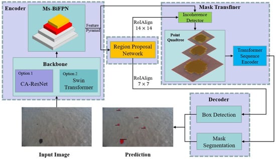
Figure 1.
The architecture of AlgaeFiner.
2.1. Encoder
The segmentation environment of floating algae is changeable and complex, compared with other image-recognition tasks. Figure 2 shows a huge difference in object features in images under different weather conditions. Some interference factors that do not exist in the training set may appear in the actual detection environment, and thus the encoder module should have strong robustness and anti-interference in the floating-algae detection task. In addition, due to the limited view of one camera, multiple cameras must be used simultaneously to monitor the whole sea area, which requires the encoder module to have a better performance without too much computational cost.
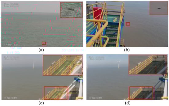
Figure 2.
The environmental variety for the floating-algae detection task. (a,b) show the floating algae in windy weather and calm weather, respectively. (c,d) show the detection conditions in sunny weather and cloudy weather, respectively.
2.1.1. CA-ResNet
The feature-extraction backbone plays an important role in the image-recognition tasks, because the robustness of features determines the performance of the model. ResNet is often used as the backbone network because of the advantages of its simple structure, fast inference-speed and no reduction of network performance due to the identity-mapping mechanism [62]. However, the ResNet cannot learn the long dependencies of images, and thus it is difficult to cope with the complex environment. Recently, the coordinate attention model has been proposed for mobile networks, by embedding the positional information into channel attention, which can help the model attend large regions with only a small computational overhead [59].
By integrating CA into the ResNet structure, a new backbone named CA-ResNet is proposed in this paper, to improve the feature-extraction ability of floating algae, and its architecture is shown in Figure 3.
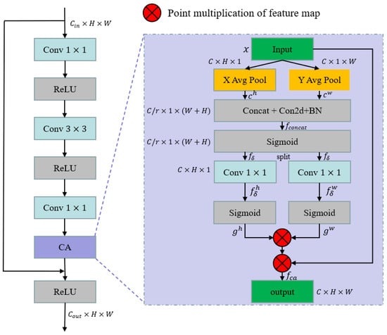
Figure 3.
The architecture of CA-ResNet in one block. ‘X Avg Pool’ and ‘Y Avg Pool’ represent the 1D horizontal global-pooling and 1D vertical global-pooling, respectively. r is the reduction ratio of channels.
Compared with the conventional bottleneck structure of ResNet, the CA-ResNet integrates the CA module before the operation of shortcut connection. Firstly, two spatial-pooling kernels (C, H, 1) or (C, 1, W) are used in parallel, to encode the position dependencies of the input features, , along the horizontal coordinate, , and the vertical coordinate, . Secondly, the and the will be concatenated in the spatial dimension to obtain the information fusion result, , and a non-linear activation operation, , will be used to encode the attention map, , in both the horizontal and vertical directions. The calculations are as follows:
where represents the convolution, is the concatenation operation and BN represents the batch normalization function.
Thirdly, is split into two separate tensors, and , and another individual Conv is applied to change the number of channels to the number of output channels. Finally, the sigmoid function is used separately on the and to calculate the correlation of the attention weights and , and the final output of the CA block, , can be calculated as follows:
2.1.2. Ms-BiFPN
As there is no unified definition on the size of floating algae, we introduce the size definition in the COCO dataset [63]. The COCO dataset is a large-scale public dataset, widely used for tasks such as object detection, semantic segmentation and instance segmentation, and has a very high application-value in the field of computer vision. The large, medium and small floating algae can be defined as follows: small size (), medium size () and large size () [63]. We visualize the floating algae of these different sizes, in Figure 4.
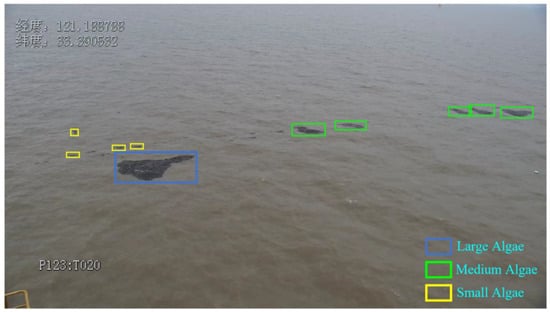
Figure 4.
The visualization of large, medium and small size floating algae.
For the fixed-position camera, the scales of floating algae will change dramatically, according to the distance from the camera. As shown in Figure 5, the targets closer to the camera tend to have a large size and strong feature-responses, while the targets far away from the camera tend to have a small size and weak feature-responses. Therefore, it is of great significance for the floating-algae detection task to utilize features under different scales, and the architecture of the modern object-detector is based on the following rules:
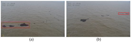
Figure 5.
The scale variety for the floating-algae detection task. (a) is the floating algae closer to the camera. (b) is the floating algae far from the camera.
- The multi-scale structure is better than the single-scale structure.
- The higher-level feature maps are more useful for detecting the large targets, while the lower-level feature maps focus on the small ones.
The conventional feature pyramid network (FPN) architecture is a top-down hierarchical network for performing information fusion on different scales, based on the feature pyramids, and its structure is shown in Figure 6a. However, the feature-fusion ability of traditional FPNs is limited by the one-way information flow. To strengthen the information exchange between different levels in the FPN, the BiFPN is proposed in [60], as shown in Figure 6b. The BiFPN replaces the conventional FPN structure with the top-down and bottom-up multi-level feature-fusion architecture, and the learnable weight-mechanism can help the model control the impact of feature responses on different scales. However, both the FPN and the BiFPN methods generate the lowest feature-map through the simple max-pooling operation. This method loses information with small responses, which may lead to the problem of missed detection in complex and highly disturbed environments. In order to overcome the shortcoming of BiFPN in floating-algae detection, Ms-BiFPN is firstly proposed in this paper, as shown in Figure 6c.
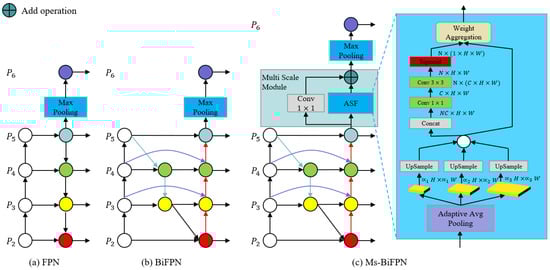
Figure 6.
The architecture of FPN, BiFPN and Ms-BiFPN. , and represent the coefficients of adaptive pooling, and the values are 0.1, 0.2 and 0.3, respectively, in this paper. N represents the number of scale factors used in adaptive pooling, and the value is 3.
The ASF is introduced in Ms-BiFPN to extract and maintain more spatial-context information in the highest-level feature maps. In ASF, we firstly use the adaptive average pooling2D operation on to generate three different context features: . Secondly, a Conv is performed on these features to reduce channels to the fixed number of 256, up-sampled to size (H, W) via bi-linear interpolation. Thirdly, the above three features are concatenated into the channel dimension, and a Conv and Conv are used sequentially to transform the number of channels from N*C to C and N, respectively. Fourthly, the sigmoid operation is applied to generate the fusion weights of three different spatial-feature maps at scales . Fifthly, the above three spatial-features are multiplied with the fusion weights to reduce the aliasing effect caused by up-sampling interpolation, and are accumulated to obtain the output of the ASF block . The calculation is as follows:
Finally, the highest-level feature map, , can be formulated as follows:
The {} will be used as input into the subsequent decoding network to obtain the bounding boxes and segmentation masks of each target.
2.2. Region Proposal Network
The RPN [52] will successively predict the potential bounding-boxes of the target on each feature-pyramid layer, and the detail of its structure is shown in Figure 7.
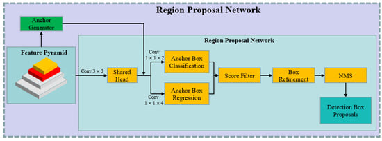
Figure 7.
The pipeline of RPN.
The predefined anchors of each pyramid layer are generated firstly in the anchor-generator block. Each pixel in the feature pyramid at different resolutions corresponds to three anchor frames with aspect ratios of 0.5, 1.0 and 2.0. Then, the shared head-block is used successively on each layer in the feature pyramid. The convolution results and the corresponding predefined anchors are fed into the box-classification branch and the box-regression branch, in parallel. In the anchor-box-classification branch, the network predicts the probability that the current anchor will belong to the foreground or the background. In the anchor-box-regression branch, the four offset values (, , and ) between the anchor box and the ground-truth box are predicted, and the calculations are as follows:
where and represent the offset of the x and y coordinates of the center point in the anchor box with respect to the ground truth. and are the offset of the width and height, respectively. and indicate the x and y coordinates of the center point of the ground-truth label. and indicate the width and heigh of the ground-truth label, respectively. and denote the predicted x and y coordinates of the anchor box’s center point, respectively. and indicate the predicted width and height of the anchor box, respectively.
Afterwards, the invalid anchor-boxes are filtered out in the score-filter block, in accordance with the score threshold, and the potential anchor boxes are refined in the box-refinement block, to ensure that all boxes do not exceed the boundary of the image. Finally, non-maximum suppression (NMS) is used on the refined boxes to obtain the final ROI proposals at different resolutions in each feature-pyramid layer.
2.3. Mask Transfiner
In the floating-algae detection task, the segmentation quality of the model is the basic task of the subsequent analysis of floating algae. However, the structures of the previous instance-segmentation methods (such as Mask R-CNN) cannot obtain the satisfactory mask-boundary results, because low-resolution feature maps are used in these networks. To address this issue in the floating-algae segmentation, the Mask-Transfiner method is introduced in this paper for high-quality mask segmentation, based on the transformer structure. The Mask Transfiner firstly locates the potential error-regions predicted for the low-resolution feature map, and then restores the accurate mask-labels at high-resolution [58]. As shown in Figure 8, the Mask-Transfiner module consists of the following four blocks: the coarse-mask-head block, the incoherence-detection block, the node-encoder block and the sequence-encoder block.
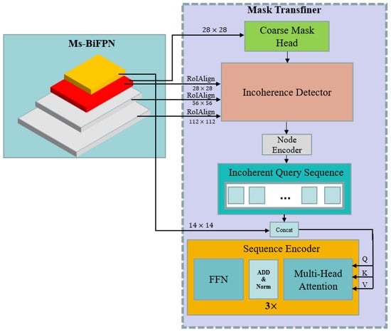
Figure 8.
The architecture of Mask Transfiner.
A coarse-mask head will be applied on the penultimate layer of the pyramid features to generate the initial coarse-mask labels with a size of .
As shown in Figure 9, the coarse-segmentation mask cannot be recovered by the up-sampling operation. The Mask Transfiner introduces the incoherent regions to identify the potential error-segmented pixels. Formally, the incoherent regions, , at scale L can be formulated as follows [58]:
where denotes the down-sampling by performing the ‘or’ operation in each neighborhood, and denotes the logical ‘exclusive or’ operation. and represent the nearest-neighbor up-sampling and down-sampling, respectively. is the binary ground-truth mask at scale level . If the original mask-value in differs from the reconstructions by at least one pixel in the next scale-level, L, the value in the corresponding position will be set to 1 in .
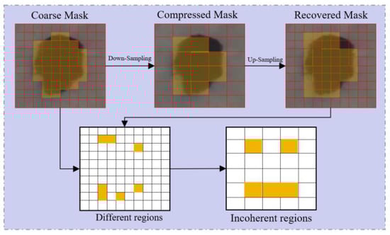
Figure 9.
The definition of incoherent regions.
Based on the above definition of incoherent regions, the incoherence-detection block [58] is introduced to locate and identify the potential error regions by constructing a multi-level, hierarchical quadtree. The higher-level feature maps (such as those with the size of ) will be up-sampled and fused with the neighboring lower-level feature maps (such as those with the size of ) sequentially, to detect the incoherent quadrant-points at different levels. Afterwards, the quadtree for all three levels will be reconstructed into the input-node sequence for the subsequent transformer-based architecture.
As each node in the input-node sequence only contains the information for potential error regions, the node-encoder block is applied to enrich the information by using the following cues [58]: (1) the region-specific and semantic information generated by the coarse-mask head. (2) The context information of surrounding neighboring points. (3) The relative-positional-encoding information to enrich the distance dependence in each level. (4) The coarsest-feature maps of the size of in Ms-BiFPN, to further enrich the semantic information of the incoherent-query sequence.
The incoherent-query sequence is fed into a 3-layer transformer-sequence encoder-block to perform both the spatial- and inter-scale-encoding operation. Each block consists of a multi-head self-attention and a fully connected feed-forward network.
As shown in Figure 10, the Mask-Transfiner method can achieve smoother and more accurate segmentation-boundaries in the Sargassum category than the Mask-R-CNN method under the same ResNet-101 backbone.
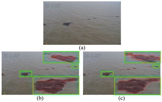
Figure 10.
The comparison between Mask R-CNN and Mask Transfiner. (a) is the source image. (b) is the Mask R-CNN result with ResNet-101. (c) is the Mask Transfiner result with ResNet-101. To better produce the performance of the network in the boundary area, we zoom in on the area in the green box.
2.4. Decoder
In order to unify the bounding boxes at different scales, the RoIAlign [57] method is proposed in Mask R-CNN, to generate feature maps of fixed sizes. The calculation of RoIAlign is as follows:
where the value of is assigned by 4, in this paper. The width and height of each bounding box are denoted as w and h, respectively. For the box- and mask-decoder heads, the bounding boxes with different resolutions are unified into the fixed sizes of and respectively, after the RoIAlign operation.
As shown in Figure 11, the box-detection branch predicts the final accurate category and position information of every bounding-box. The 2D-feature maps are firstly flattened into a 1D dimension, and fed into two parallel branches. The upper branch can predict the final exact position-coordinates of the target, and the lower branch can obtain the final classification-category of the target.
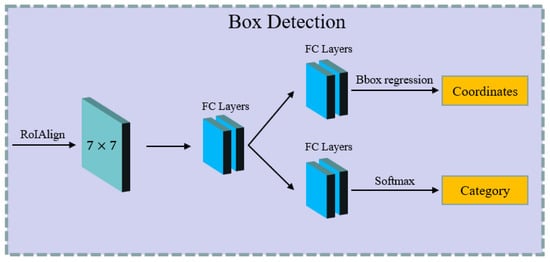
Figure 11.
The pipeline of the box-detection branch.
The architecture of the mask-segmentation branch is shown in Figure 12. In order to retain more details of the floating algae, the pooling size used in RoIAlign is . The segmentation-head branch uses four connected convolution- and ReLU-operations to filter the input-feature map, and the kernel size and stride in each convolution block are and 1, respectively. Then, the size of the feature map is increased to through the ConvTranspose2d operation. Afterward, a convolution-operation with output channels is applied to classify all pixels in the feature map. Finally, the probability feature-map is up-sampled to the original image size, to obtain the final segmentation results of the floating algae.
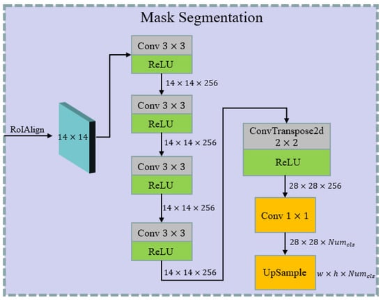
Figure 12.
The architecture of the mask-segmentation branch. indicates the number of classes. w and h represent the original image’s width and height, respectively.
2.5. Loss Function
A multi-task loss [58] is introduced into our AlgaeFiner during the training phase, formed as follows:
where the represents the bounding-box-position regression- and classification-losses from the box-detection head in the decoder. The box-position regression loss describes the error between the offset of the prediction bounding-boxes and the ground truth. The classification loss describes the error between the predicted category and the real category. The is the loss of the coarse-mask labels generated by the coarse-mask head, and it can also represent the loss value in the traditional instance-segmentation methods (such as Mask R-CNN). The and represent the predicted labels-loss for incoherent nodes and the incoherent region detection-loss in the Mask Transfiner module, respectively. The hyper-parameter values of are {1.0, 1.0, 1.0, 0.5} in this paper.
2.6. Datasets
In accordance with the location of the green-tide and gold-tide outbreak areas in the East China Sea in recent years, we collected the RGB-image data from the surveillance videos on ships and shores from 2020 to 2022. As shown in Table 1, we present 7 camera positions in Nantong and Yancheng in the Jiangsu sea area

Table 1.
Camera position for surveillance adopted in the East China Sea for our paper.
The dataset, including 3600 labeled RGB images with a resolution of 1920 × 1080, has two manually labeled categories of Ulva prolifera and Sargassum. We divided 3000 images from the dataset into training and testing, with 600 for testing.
3. Results
3.1. Evaluation Metrics
In this section, the following metrics: average precision (AP), average recall (AR) and average boundary precision () [64] will be used to evaluate the performance of our AlgaeFiner and other instance-segmentation models.
The AP and AR are the average values of precision (P) and recall (R), and can be calculated as follows:
where n represents the number of categories, and its value is 2 (Ulva Prolifera and Sargassum) in our paper. and indicate the precision and recall, respectively, for category i,. TP, FP and FN represent the true positive, the false positive and the false negative, respectively.
From (15), we can draw the following conclusions: (1) the higher the value of AP, the lower the false-detection rate of the model. (2) The higher the value of AR, the lower the missed-detection rate of the model.
However, the single AP and AR metrics make it difficult to accurately evaluate the segmentation quality of the mask boundary. The metric will be introduced in our paper to provide a more accurate analysis of algae-segmentation results. The [64] is calculated as follows:
where represents the set of pixels whose distance from the ground-truth mask is not greater than d, and represents the set of pixels whose distance from the prediction mask is not greater than d. The GT and Pre represent the ground-truth binary mask and the prediction binary mask, respectively; d is the pixel width of the boundary region, and its value is usually set to 0.5% of an image diagonal.
In addition, the following metrics and definitions will be used in our paper simultaneously, to analyze the performance of the model in segmenting the algae at different sizes, as shown in Table 2.
Table 2.
The definition of AP, AR and at different sizes.
Where , and represent the average precision, average recall and average boundary precision for the large size, respectively, and the other metric definitions for the medium and small sizes are the same as those for the large size.
3.2. Experimental Setups
The AlgaeFiner is implemented in the following environments: PyTorch v1.9.1, Detectron2 v0.5, CUDA v11.4 and cuDNN v11.4 on four NVIDIA TITAN RTX GPU with 24 GB memory. During the training phase, we use the random flip, center crop, image normalization and contrast variation as data-augmentation methods. The model configurations and the other training hyper-parameters are shown in Table 3. In the backbone configurations, the C-R50 + FPN indicates that the model selects the coordinate attention ResNet-50 (R50) as the feature-extraction backbone and FPN as the feature-fusion network. The meaning of other configurations in the backbone are the same as C-R50 + FPN. The Swin-T represents the Swin Transformer with a tiny backbone, and the meaning of Swin-B is same as Swin-T.
Table 3.
Model configurations and training hyper-parameters.
3.3. Evaluation of Model Performance
As shown in Figure 13, we use the AlgaeFiner with C-R101 and Ms-BiFPN as examples to analyze the changes of loss as described in Section 2.5, during the training phase. We chose the scatter diagram with dense sampling to see more details of the changes in the total loss. We used the broken line to describe the remaining losses. With the increasing iterations, all losses show an overall downward trend. Since the total number of categories of our floating-algae detection task is relatively small, the box-classification loss drops fastest and tends to become stable at approximately 20,000 iterations. Meanwhile, the descend speed of the coarse-mask loss is the slowest, and is still at a high level when the training stage is finished. This means that it is difficult for traditional instance-segmentation methods to obtain better mask results in the floating-algae detection task. By introducing the Mask Transfiner method in our AlgaeFiner, the refine-mask loss presents a smooth downward trend, and finally stabilizes at a lower value.
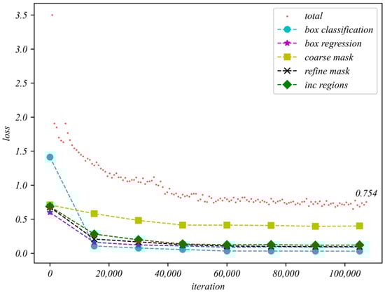
Figure 13.
The loss in the training phase based on the AlgaeFiner with C-R101 + Ms-BiFPN.
In this section, we will compare the performance of Mask R-CNN [57], Mask Transfiner [58] and our AlgaeFine on the above metrics under different configurations, as shown in Table 4, Table 5 and Table 6. The Mask R-CNN is the pioneer of the instance-segmentation method, and has achieved great success in many visual-recognition fields. The Mask Transfiner improves the segmentation accuracy effectively, based on the Mask R-CNN architecture. By comparing the above methods under different configurations, the performance evaluation of AlgaeFiner can be fully conducted.
Table 4.
Comparison performance of different models on AP.
Table 5.
Comparison performance of different models on AR.
Table 6.
Comparison performance of different models on .
In Table 4 and Table 5, we compare the performance of different models under the AP and AR metrics. Obviously, the AlgaeFiner with the Swin-B backbone can obtain better results, while the Mask R-CNN with the R50 backbone is relatively worse.
Compared to the Mask Tansfiner and AlgaeFiner under the Swin-B backbone in Table 4 and Table 5, the AlgaeFiner has a 2.62% and 1.87% improvement in the and , respectively, and a 4.11% and 4.73% improvement in the and , respectively. The improvement in the AR metrics is greater than that in the AP metrics, which means the missed-detection rate has been significantly reduced by replacing the conventional FPN module with the Ms-BiFPN module, under the same backbone network. Since both coordinate attention and the Ms-BiFPN are integrated into the AlgaeFiner, the performance improvement in the ResNet structure is higher than in the Swin Transformer architecture. For the ResNet-101 backbone, the AlgaeFiner has a 3.87% and 5.17% improvement in the and , respectively, when compared with the Mask R-CNN.
In Table 4 and Table 5, the AlgaeFiner with the Swin-B backbone can obtain the best performance in different algae sizes compared with other instance-segmentation methods. For small algae, the and decline significantly in the Mask Transfiner and Mask R-CNN. Meanwhile, compared with the and , the AlgaeFiner with the Swin-B backbone has only a 4.34% and 5.72% decline in the and , respectively. In addition, the segmentation performance of all models for medium and large algae-sizes are better than the average values.
Compared with the results of C-R101 and Swin-B in our AlgaeFiner, we can find that the Swin-B can reach the higher and in Table 4. This means the Swin Transformer backbone has a stronger anti-interference ability in the ocean than C-R101, by efficiently modeling the long-range dependencies of floating algae in images, which can reduce the rate of false segmentation in the complex marine-scenes. However, the C-R101 backbone has a 1.54% and 1.46% improvement in comparison with the Swin-B in the and , respectively, as shown in Table 5.
From Table 6, it is clear that all models have declined significantly in , compared with the . From the perspective of the results at different sizes, the performance for large and medium algae suffers the most performance degradation, which means the and find it difficult to accurately evaluate the performance of the model on medium and large algae. It is mainly because the Mask IoU method used on the AP metrics treats all pixels equally, resulting in less sensitivity to boundary quality at medium and large algae-size. Our AlgaeFiner with a C-R101 structure can obtain the best result (36.32%) for the small algae and the Swin-B structure can achieve the best results (53.23% and 27.75%) for the medium and large algae. Compared with the Mask R-CNN method, the Mask Transfiner and our AlgaeFiner can achieve a significant improvement on the metrics, because the error-segmentation pixels on the boundary are corrected by the Mask Transfiner module. Taking the R101 and C-R101 as examples, the Mask Transfiner and AlgaeFiner can obtain a 4.64% and 6.52% improvement, respectively, in , compared with the Mask R-CNN.
In Figure 14, Figure 15, Figure 16, Figure 17, Figure 18 and Figure 19, we visually compare the segmentation results of floating algae in different sample scenes. The meaning of (a)–(l) in the figures below are as follows: (a) is the source image, (b) is the ground truth, (c) is the AlgaeFiner with Swin-B, (d) is the AlgaeFiner with Swin-T, (e) is the AlgaeFiner with C-R101, (f) is the AlgaeFiner with C-R50, (g) is the Mask Transfiner with Swin-B, (h) is the Mask Transfiner with Swin-T, (i) is the Mask Transfiner with R101, (j) is the Mask Transfiner with R50, (k) is the Mask R-CNN with R101, and (l) is the Mask R-CNN with R50. The areas depicted in the green color represent the category of Ulva Prolifera and the yellow areas represent the category of Sargassum. The scene of Ulva Prolifera is shown in Figure 14, Figure 15 and Figure 16, and the scene of Sargassum is shown from Figure 17, Figure 18 and Figure 19. In addition, in order to better show the experimental details, we enlarged the areas of red and yellow boxes in the above section of each image.
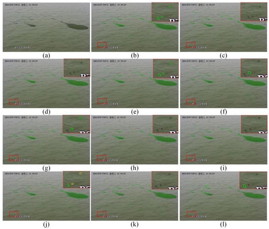
Figure 14.
The visual comparison of results of different models in scene 1.
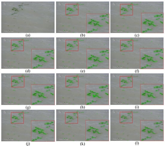
Figure 15.
The visual comparison of results of different models in scene 2.
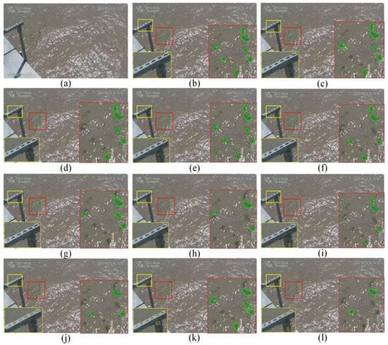
Figure 16.
The visual comparison of results of different models in scene 3.
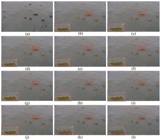
Figure 17.
The visual comparison of results of different models in scene 4.
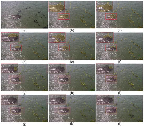
Figure 18.
The visual comparison of results of different models in scene 5.
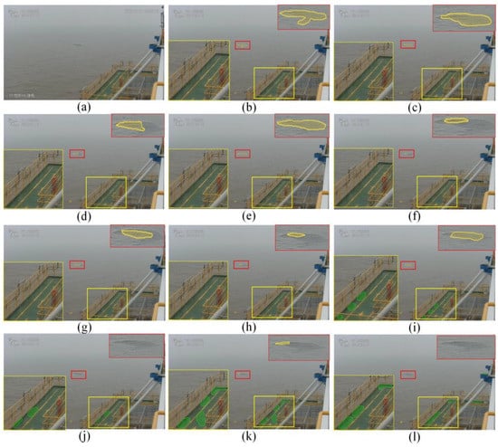
Figure 19.
The visual comparison of results of different models in scene 6.
Combined with the AR metrics in Table 3 and Figure 14c–f, we can see clearly that the AlgaeFiner based on the ResNet (C-R101 and C-R50) has a higher segmentation rate for small targets than the Swin Transformer architectures (Swin-B and Swin-T).
Compared with AlgaeFiner and Mask TransFiner (red box areas) in Figure 15 and Figure 17, the segmentation results of Mask R-CNN on the categories of Ulva Prolifera and Sargassum are coarse and incomplete. For the category of Sargassum of medium and large size in Figure 18k,l, the boundary-segmentation results of Mask R-CNN are contracted inward and are inaccurate, because the mask prediction is based on the features with low resolution. In Figure 18c–j, by introducing the quadtree mask-transfiner module, the potential error-boundary pixels can be refined in the features with high resolution, so that the boundary-segmentation accuracy of the Mask Transfiner and AlgaeFiner are greatly improved.
In addition, all methods based on the ResNet (R101 and R50) structures, including Mask Transfiner and Mask R-CNN, have false detection in the yellow-box areas in Figure 16 and Figure 19, because of the existence of some strong interference areas with similar features to the floating algae, in the scenes. In order to overcome the problem of false detection in complex scenes, the coordinate-attention mechanism is introduced in our AlgaeFiner to capture the long-range dependencies in both the channel- and position-dimension, which can help the ResNet structure model to study the feature representation of algae effectively and accurately. Therefore, our AlgaeFiner with the C-R101 and C-R50 backbone has less false-detection of floating algae, even if there are some similar targets on the ocean.
Comparing the red-box areas in Figure 18, it is obvious that all models have the problem of missed detection because of the reflection interference of strong sunlight. On the one hand, the sunlight changes the features of floating algae, leading to the missed detection in the model. On the other hand, from the perspective of large-algae segmentation, due to the huge information loss in the highest-level feature maps, the problem of missed detection in models with FPN structures is more serious than in models with Ms-BiFPN structures. For the floating-algae-segmentation task, the performance of large algae mainly depends on the highest-level feature map. However, both FPN and BiFPN have the problem of feature-response loss, because of the max-pooling operation. By replacing the FPN with the Ms-BiFPN, the performances of big algae segmentation in AlgaeFiner are superior to those of other models, as see in Figure 18c–f.
3.4. Ablation Study
3.4.1. Impact of Input Resolution
To further discuss the influence of input-image resolution on the performance of floating-algae segmentation in our proposed networks, we compare the variation metrics under different input-resolutions, in Table 7.
Table 7.
The variation of , , and inference time under different resolutions.
With the resolution increasing, the AR metrics under different configurations are all improved, which means the image resolution has a great impact on the missed detection. However, the AP metrics show a trend of rising first and then declining. Specifically, when the input resolution is improved from 960 × 540 to 1920 × 1080, the of Swin-B is increased by 4.66% () and the C-R101 is increased by 2.42% (). When the input resolution is improved from 1920 × 1080 to 3840 × 2160, both the and are decreased for all configurations. The Swin-B has a 1.17% () and 0.85% decline (), respectively, and the C-R101 has a 0.71% () and 1.36% () decline, respectively.
This indicates that the improvement in resolution cannot successfully reduce the false detection of the model. With the increase in input resolution, the size of the feature pyramid will also be enlarged. This is favorable for the improvement of AR metrics, because some weak responses can be retained in the feature maps with high resolution. However, it is also unfavorable for AP metrics, as some interference responses will still be retained in the high-semantic-feature maps with high resolution, and these responses may be discarded in the high-semantic-feature maps with low resolution. These interference responses will eventually lead to the increases in the false-detection rate, thus resulting in the decline of AP metrics.
Meanwhile, the inference time of our model will be increased dramatically with the improvement of input resolution, as shown in Table 7. The inference time based on the ResNet structure is obviously higher than that based on the Swin-Transformer structure. For the resolution of 1920 × 1080, the inference time of C-R101 is twice that of Swin-B, while the C-R101 has only a 1.39% and 0.39% decline in the and , respectively. Considering the performance and speed under different configurations and resolutions, the AlgaeFiner based on the C-R101 backbone is the best choice for the floating-algae detection task under the input resolution of 1920 × 1080.
3.4.2. Impact of the Coordinate Attention
The coordinate-attention module is a lightweight attention-mechanism, which is used to help the model to solve the problem of “what” and “where” in the image. In this section, we will further discuss the impact of coordinate attention. Based on our AlgaeFiner architecture, we replaced the Coordinate ResNet with the conventional ResNet, and the comparison results are shown in Table 8.
Table 8.
The comparison of , , and under different backbones.
By removing the coordinate attention mechanism in the ResNet structure, the AP and AR metrics all decline in the R50 and R101 structures. Compared with the C-R101 structure, the R101 has a 3.42% and 3.58% decline in the and , respectively, and the and also decline by 0.61% and 0.92%, respectively. Obviously, the decline ratio of AP metrics is greater than that of AR metrics. After removing the coordinate attention mechanism, the AlgaeFiner with the conventional ResNet can only capture the local relations (such as color- or shape-relation), which will lead to the problem of false detection in complex scenes. As shown in the yellow areas in Figure 20, due to the similarity with the Sargassum category (such as color and shape), the R50 and R101 will detect the rusty railings as Sargassum.
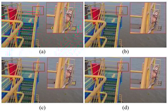
Figure 20.
The comparison of ResNet and Coordinate ResNet in AlgaeFiner. (a) is the AlgaeFiner with R50, (b) is the AlgaeFiner with C-R50, (c) is the AlgaeFiner with R101, (d) is the AlgaeFiner C-R101.
3.4.3. Impact of the Ms-BiFPN
In instance-segmentation methods, it is important for the performance of the model to make full use of features under different scales. In this section, we will compare the influence of the Ms-BiFPN, BiFPN and FPN modules.
From Table 9, it is clear that the Ms-BiFPN can obtain the best results in all AP and AR metrics, compared with the other two fusion-strategies. Meanwhile, the influence of fusion strategies on AR metrics is greater than on the AP metrics. Taking the C-R101 as an example, the and have improved by 3.75% (%) and 4.37% (%), respectively, by replacing the FPN with the BiFPN. However, when we replace the BiFPN with the Ms-BiFPN, the improvement in the AR metrics (, ) is not significant. This is because the improvement in Ms-BiFPN is mainly reflected in the large algae sizes rather than in the average level. In Figure 21, based on the C-R101 structure, we compare the AP and AR results of the above three different fusion-strategies for every definition of algae size.
Table 9.
The comparison of , , and under different feature-fusion strategies.
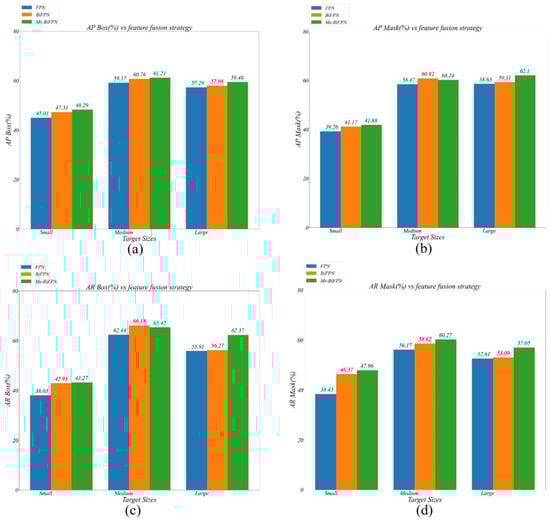
Figure 21.
The comparison of AP and AR metrics under different algae size: (a) are the results of AlgaeFiner in AP box under the different fusion strategies, (b) are the results of AlgaeFiner in AP mask under the different fusion strategies, (c) are the results of AlgaeFiner in AR box under the different fusion strategies, and (d) are the results of AlgaeFiner in AR mask under the different fusion strategies.
Both the BiFPN and the Ms-BiFPN can achieve a slight improvement on the FPN method in AP metrics. Compared with FPN in the AR metrics, the BiFPN can reach a better performance for the small and medium size, but it is difficult to obtain satisfactory results for the large size. Therefore, by replacing the single top-down hierarchical structure with a bidirectional cross-scale structure, the BiFPN can effectively improve the segmentation performance on small- and medium-sized algae. However, from the perspective of the large algae, the BiFPN has only a 0.48% and 0.36% improvement in the and , respectively, compared with the FPN method. It indicates that the loss of information in the top-level feature map has a crucial impact on the large-algae segmentation.
To further improve the segmentation performance of the model on large-sized algae, the Ms-BiFPN is proposed, replacing the max-pooling operation with the multi-scale module. In Figure 21, the performance for large algae has improved by 3.96% and 6.1% in the and respectively, compared with the BiFPN method.
4. Discussion
Our method, a novel deep-learning model named AlgaeFiner for floating-algae detection, integrates the object-detection task and the mask-segmentation task into a unified network, which can not only output the external bounding-box of each target, but also obtain the accurate segmentation-area within the same category. To reduce the interference of a complex marine-environment, a novel feature-extraction backbone named CA-ResNet is proposed, by integrating the coordinate-attention mechanism into the conventional ResNet structure. The long-range dependencies between different channels and positions can be modeled simultaneously, which can effectively reduce the false segmentation. Meanwhile, the computation performance of CA-ResNet can also satisfy the real-time requirements of marine monitoring. The Ms-BiFPN module is proposed for solving the problem of large-scale changing by embedding the multi-scale block into the BiFPN structure. The ASF block is integrated into the multi-scale module to extract more spatial-context information in the highest-level feature maps. The performance of large algae detection is greatly improved by replacing the conventional BiFPN structure with the Ms-BiFPN structure. The transformer-based module named Mask Transfiner is introduced to improve the boundary-segmentation quality of AlgaeFiner. A multi-level hierarchical-point quadtree is built to detect the potential error-segmented pixels in the coarse masks at different scales, and a multi-head self-attention block is applied to predict the final refined mask-labels.
From the experimental results, we find that the AlgaeFiner has achieved a relatively good performance for floating-algae segmentation under different real-application scenarios on the sea. We also take the interference of bad weather into account in evaluating our model, although this is not the focus point of our model. By collecting and analyzing the surveillance-video data on ships and shores in recent years, we summarize the following different situations in the floating-algae detection task: rainy, sun reflection, cloudy, foggy and wave. The results of AlgaeFiner in the above environments are shown in Figure 22 and Figure 23. In Figure 22d and Figure 23f,h, it is clear that the AlgaeFiner can perform well in some bad-weather scenes with obvious floating algae.
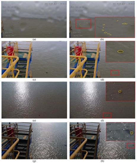
Figure 22.
The results of AlgaeFiner in rainy and sun reflection scenes: (a,c) are the rainy scene, and (e,g) are the sun-reflection scene, and (b,d,f,h) indicate the detection results of AlgaeFiner corresponding to the images (a,c,e,g).
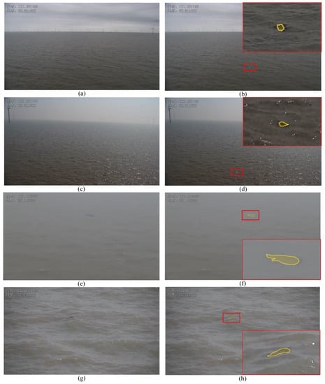
Figure 23.
The results of AlgaeFiner in cloudy, foggy and wave scenes: (a,c) are the cloudy scene, (e) is the foggy scene, (g) is the wave scene, and (b,d,f,h) are the results of the images (a,c,e,g).
However, in Figure 22b, due to the blur of the camera lens caused by raindrops, the detection performance of AlgaeFiner declined (missed detection). On the one hand, the rain occlusion leads to information loss in the feature-extraction phase, which cannot be solved by our proposed feature-extraction structure (CA-ResNet). On the other hand, although the Ms-BiFPN can improve the detection ability for small targets, the AlgaeFiner will still miss detection of the floating algae in the situation where the target feature is unobvious and there exists strong interference in the scene, simultaneously.
In Figure 22f,h and Figure 23b,d, although the AlgaeFiner has detected the floating algae targets, the areas-of-segmentation results are still incomplete and inaccurate. In these scenes, the feature responses extracted by our network are always weak, and the Mask Transfiner module cannot effectively improve the accuracy and integrity of mask-segmentation results under the weak feature-responses.
Above all, although our method considers the influence of different environmental factors, it still has some shortcomings in dealing with bad weather, due to the limited amount of marine-environment data. In a further study, on the one hand we will explore the robustness of our model under marine scenes of different weather conditions. On the other hand, we will further research the possibility of introducing spectral data into marine-pollution monitoring.
5. Conclusions
Floating-algae detection is a difficult research topic in the field of image recognition, due to the complexity of the sea environment. In this paper, we proposed a novel instance-segmentation network named AlgaeFiner for high-quality floating-algae detection based on the surveillance RGB-images captured from the cameras on ships and shores. The performance evaluation of different instance-segmentation methods at different real marine-scenes are performed.
For high-quality segmentation of floating algae, we introduce Mask Transfiner to locate the potential error pixels on a low-resolution feature map, and refine the accurate segmentation-regions at high-resolution. Meanwhile, we propose the CA-ResNet to extract the feature of floating algae effectively by building the long-range dependencies between different channels and positions at the same time. The Ms-BiFPN module is designed to control the impact of feature responses at different scales, using the multi-scale block, and achieving more spatial-context information using the ASF block.
The extensive experiment results show that our proposed AlgaeFiner can achieve better segmentation performance with a lower computation cost compared with other state-of-the-art instance-segmentation methods. The AlgaeFiner with the C-R101 and Ms-BiFPN configuration can achieve 45.39% and 48.63% in the AP_mask and AP_box, respectively, compared with other instance-segmentation methods. Therefore, our AlgaeFiner can achieve high application-value in the floating-algae monitoring task.
Author Contributions
Methodology, L.W.; software, L.Z.; validation, K.C.; formal analysis, Y.G.; data curation, K.C.; writing—original draft preparation, Y.Z.; writing—review and editing, L.W.; project administration, X.W. All authors have read and agreed to the published version of the manuscript.
Funding
This thesis is supported by the funding from the Key Laboratory of Marine Ecological Monitoring and Restoration Technologies, MNR: MEMRT202209, and funding from the Technology Innovation Center for Ocean Telemetry, Ministry of Natural Resources: 006.
Data Availability Statement
Not applicable.
Acknowledgments
The authors would like to thank the editors and the reviewers for their valuable suggestions.
Conflicts of Interest
The authors declare no conflict of interest.
References
- Anderson, C.R.; Moore, S.K.; Tomlinson, M.C.; Silke, J.; Cusack, C.K. Living with harmful algal blooms in a changing world: Strategies for modeling and mitigating their effects in coastal marine ecosystems. Coast. Mar. Hazards Risks Disasters 2015, 17, 495–561. [Google Scholar]
- Xiao, J.; Wang, Z.; Liu, D.; Fu, M.; Yuan, C.; Yan, T. Harmful macroalgal blooms (HMBs) in China’s coastal water: Green and golden tides. Harmful Algae 2021, 107, 102061. [Google Scholar] [CrossRef] [PubMed]
- Qi, L.; Hu, C.; Shang, S. Long-term trend of Ulva prolifera blooms in the western Yellow Sea. Harmful Algae 2016, 58, 35–44. [Google Scholar] [CrossRef] [PubMed]
- Ye, N.; Zhang, X.; Mao, Y.; Liang, C.; Xu, D.; Zou, J.; Zhuang, Z.; Wang, Q. ‘Green tides’ are overwhelming the coastline of our blue planet: Taking the world’s largest example. Environ. Res. 2011, 26, 477–485. [Google Scholar] [CrossRef]
- Xing, Q.G.; Wu, L.L.; Tian, L.Q.; Cui, T.W.; Li, L.; Kong, F.Z.; Gao, X.L.; Wu, M.Q. Remote sensing of early-stage green tide in the Yellow Sea for floating-macroalgae collecting campaign. Mar. Pollut. Bull. 2018, 133, 150–156. [Google Scholar] [CrossRef]
- Chen, Y.; Sun, D.; Zhang, H.; Wang, S.; Qiu, Z.; He, Y. Remote-sensing monitoring of green tide and its drifting trajectories in Yellow Sea based on observation data of geostationary ocean color imager. Acta Opt. Sin. 2020, 40, 0301001. [Google Scholar] [CrossRef]
- Lu, T.; Lu, Y.C.; Hu, L.B.; Jiao, J.N.; Zhang, M.W.; Liu, Y.X. Uncertainty in the optical remote estimation of the biomass of Ulva prolifera macroalgae using MODIS imagery in the Yellow Sea. Opt. Express 2019, 27, 18620–18627. [Google Scholar] [CrossRef]
- Hu, L.B.; Zheng, K.; Hu, C.; He, M.X. On the remote estimation of Ulva prolifera areal coverage and biomass. Remote Sens. Environ. 2019, 223, 194–207. [Google Scholar] [CrossRef]
- Cao, Y.Z.; Wu, Y.; Fang, Z.; Cui, X.; Liang, J.; Song, X. Spatiotemporal patterns and morphological characteristics of Ulva prolifera distribution in the Yellow Sea, China in 2016–2018. Remote Sens. 2019, 11, 445. [Google Scholar] [CrossRef]
- Xing, Q.G.; An, D.; Zheng, X.; Wei, Z.; Wang, X.; Li, L.; Tian, L.; Chen, J. Monitoring seaweed aquaculture in the Yellow Sea with multiple sensors for managing the disaster of macroalgal blooms. Remote Sens. Environ. 2019, 231, 111279. [Google Scholar] [CrossRef]
- Xing, Q.G.; Guo, R.; Wu, L.; An, D.; Cong, M.; Qin, S.; Li, X. High-resolution satellite observations of a new hazard of golden tides caused by floating Sargassum in winter in the Yellow Sea. IEEE Geosci. Remote Sens. Lett. 2017, 14, 1815–1819. [Google Scholar] [CrossRef]
- Xu, F.X.; Gao, Z.Q.; Shang, W.T.; Jiang, X.P.; Zheng, X.Y.; Ning, J.C.; Song, D.B. Validation of MODIS-based monitoring for a green tide in the Yellow Sea with the aid of unmanned aerial vehicle. J. Appl. Remote Sens. 2017, 11, 012007. [Google Scholar] [CrossRef]
- Shin, J.S.; Lee, J.S.; Jiang, L.H.; Lim, J.W.; Khim, B.K.; Jo, Y.H. Sargassum Detection Using Machine Learning Models: A Case Study with the First 6 Months of GOCI-II Imagery. Remote Sens. 2021, 13, 4844. [Google Scholar] [CrossRef]
- Cui, T.W.; Li, F.; Wei, Y.H.; Yang, X.; Xiao, Y.F.; Chen, X.Y.; Liu, R.J.; Ma, Y.; Zhang, J. Super-resolution optical mapping of floating macroalgae from geostationary orbit. Appl. Opt. 2020, 59, C70–C77. [Google Scholar] [CrossRef]
- Liang, X.J.; Qin, P.; Xiao, Y.F. Automatic remote sensing detection of floating macroalgae in the yellow and east china seas using extreme learning machine. J. Coast. Res. 2019, 90, 272–281. [Google Scholar] [CrossRef]
- Qiu, Z.F.; Li, Z.; Bila, M.; Wang, S.; Sun, D.; Chen, Y. Automatic method to monitor floating macroalgae blooms based on multilayer perceptron: Case study of Yellow Sea using GOCI images. Opt. Express 2018, 26, 26810–26829. [Google Scholar] [CrossRef]
- Geng, X.M.; Li, P.X.; Yang, J.; Shi, L.; Li, X.M.; Zhao, J.Q. Ulva prolifera detection with dual-polarization GF-3 SAR data. IOP Conf. Ser. Earth Environ. Sci. 2020, 502, 012026. [Google Scholar] [CrossRef]
- Wu, L.; Wang, L.; Min, L.; Hou, W.; Guo, Z.; Zhao, J.; Li, N. Discrimination of algal-bloom using spaceborne SAR observations of Great Lakes in China. Remote Sens. 2018, 10, 767. [Google Scholar] [CrossRef]
- Cui, T.W.; Liang, X.J.; Gong, J.L.; Tong, C.; Xiao, Y.F.; Liu, R.J.; Zhang, X.; Zhang, J. Assessing and refining the satellite-derived massive green macro-algal coverage in the Yellow Sea with high resolution images. ISPRS J. Photogramm. Remote Sens. 2018, 144, 315–324. [Google Scholar] [CrossRef]
- Kislik, C.; Dronova, I.; Kelly, M. UAVs in support of algal bloom research: A review of current applications and future opportunities. Drones 2018, 2, 35. [Google Scholar] [CrossRef]
- Jang, S.W.; Yoon, H.J.; Kwak, S.N.; Sohn, B.Y.; Kim, S.G.; Kim, D.H. Algal Bloom Monitoring using UAVs Imagery. Adv. Sci. Technol. Lett. 2016, 138, 30–33. [Google Scholar]
- Jung, S.; Cho, H.; Kim, D.; Kim, K.; Han, J.I.; Myung, H. Development of Algal Bloom Removal System Using Unmanned Aerial Vehicle and Surface Vehicle. IEEE Access 2017, 5, 22166–22176. [Google Scholar] [CrossRef]
- Kim, H.-M.; Yoon, H.-J.; Jang, S.W.; Kwak, S.N.; Sohn, B.Y.; Kim, S.G.; Kim, D.H. Application of Unmanned Aerial Vehicle Imagery for Algal Bloom Monitoring in River Basin. Int. J. Control Autom. 2016, 9, 203–220. [Google Scholar] [CrossRef]
- Cheng, K.H.; Chan, S.N.; Lee, J.H.W. Remote sensing of coastal algal blooms using unmanned aerial vehicles (UAVs). Mar. Pollut. Bull. 2020, 152, 110889. [Google Scholar] [CrossRef]
- Arellano-Verdejo, J.; Lazcano-Hernández, H.E. Collective view: Mapping Sargassum distribution along beaches. PeerJ Comput. Sci. 2021, 7, e528. [Google Scholar] [CrossRef]
- Valentini, N.; Yann, B. Assessment of a smartphone-based camera system for coastal image segmentation and sargassum monitoring. J. Mar. Sci. Eng. 2020, 8, 23. [Google Scholar] [CrossRef]
- Arellano-Verdejo, J.; Santos-Romero, M.; Lazcano-Hernandez, H.E. Use of semantic segmentation for mapping Sargassum on beaches. PeerJ 2022, 10, e13537. [Google Scholar] [CrossRef]
- Pan, B.; Shi, Z.; An, Z.; Jiang, Z.; Ma, Y. A novel spectral-unmixing-based green algae area estimation method for GOCI data. IEEE J. Sel. Top. Appl. Earth Obs. Remote Sens. 2016, 10, 437–449. [Google Scholar] [CrossRef]
- Wang, M.Q.; Hu, C.M. Mapping and quantifying Sargassum distribution and coverage in the Central West Atlantic using MODIS observations. Remote Sens. Environ. 2016, 183, 350–367. [Google Scholar] [CrossRef]
- Wang, M.; Hu, C. Automatic extraction of Sargassum features from sentinel-2 msi images. IEEE Trans. Geosci. Remote Sens. 2020, 59, 2579–2597. [Google Scholar] [CrossRef]
- Ody, A.; Thibaut, T.; Berline, L. From In Situ to satellite observations of pelagic Sargassum distribution and aggregation in the Tropical North Atlantic Ocean. PLoS ONE 2019, 14, e0222584. [Google Scholar] [CrossRef] [PubMed]
- Shen, H.; Perrie, W.; Liu, Q.; He, Y. Detection of macroalgae blooms by complex SAR imagery. Mar. Pollut. Bull. 2014, 78, 190–195. [Google Scholar] [CrossRef] [PubMed]
- Ma, Y.F.; Wong, K.P.; Tsou, J.Y.; Zhang, Y.Z. Investigating spatial distribution of green-tide in the Yellow Sea in 2021 using combined optical and SAR images. J. Mar. Sci. Eng. 2022, 10, 127. [Google Scholar] [CrossRef]
- Jiang, X.; Gao, M.; Gao, Z. A novel index to detect green-tide using UAV-based RGB imagery. Estuar. Coast. Shelf Sci. 2020, 245, 106943. [Google Scholar] [CrossRef]
- Xu, F.; Gao, Z.; Jiang, X.; Shang, W.; Ning, J.; Song, D.; Ai, J. A UAV and S2A data-based estimation of the initial biomass of green algae in the South Yellow Sea. Mar. Pollut. Bull. 2018, 128, 408–414. [Google Scholar] [CrossRef]
- Ronneberger, O.; Philipp, F.; Thomas, B. U-net: Convolutional networks for biomedical image segmentation. In Proceedings of the International Conference on Medical Image Computing and Computer-Assisted Intervention, Munich, Germany, 5–9 October 2015; pp. 234–241. [Google Scholar]
- Zhao, Z.Q.; Zheng, P.; Xu, S.; Wu, X. Object detection with deep learning: A review. IEEE Trans. Neural Netw. Learn. Syst. 2019, 30, 3212–3232. [Google Scholar] [CrossRef]
- Li, X.F.; Liu, B.; Zheng, G.; Ren, Y.; Zhang, S.; Liu, Y.; Zhang, B.; Wang, F. Deep-learning-based information mining from ocean remote-sensing imagery. Natl. Sci. Rev. 2020, 7, 1584–1605. [Google Scholar] [CrossRef]
- Wan, X.C.; Wan, J.H.; Xu, M.M.; Liu, S.W.; Sheng, H.; Chen, Y.L.; Zhang, X.Y. Enteromorpha coverage information extraction by 1D-CNN and Bi-LSTM networks considering sample balance from GOCI images. IEEE J. Sel. Top. Appl. Earth Obs. Remote Sens. 2021, 14, 9306–9317. [Google Scholar] [CrossRef]
- Kim, S.M.; Shin, J.; Baek, S.; Ryu, J.H. U-Net convolutional neural network model for deep red tide learning using GOCI. J. Coast. Res. 2019, 90, 302–309. [Google Scholar] [CrossRef]
- Guo, Y.; Le, G.; Li, X.F. Distribution Characteristics of Green Algae in Yellow Sea Using an Deep Learning Automatic Detection Procedure. In Proceedings of the 2021 IEEE International Geoscience and Remote Sensing Symposium IGARSS, Brussels, Belguim, 11–16 July 2021; pp. 3499–3501. [Google Scholar]
- Zhao, X.; Liu, R.; Ma, Y.; Xiao, Y.; Ding, J.; Liu, J.; Wang, Q. Red Tide Detection Method for HY–1D Coastal Zone Imager Based on U−Net Convolutional Neural Network. Remote Sens. 2021, 14, 88. [Google Scholar] [CrossRef]
- Yabin, H.U.; Yi, M.A.; Jubai, A.N. Research on High Accuracy Detection of Red Tide Hyperspecrral Based on Deep Learning CNN. Int. Arch. Photogramm. Remote Sens. Spat. Inf. Sci. 2018, 42, 3. [Google Scholar]
- Hong, S.M.; Baek, S.S.; Yun, D.; Kwon, Y.H.; Duan, H.; Pyo, J.C.; Cho, K.H. Monitoring the vertical distribution of HABs using hyperspectral imagery and deep learning models. Sci. Total Environ. 2021, 794, 148592. [Google Scholar] [CrossRef] [PubMed]
- Wang, S.K.; Liu, L.; Yu, C.; Sun, Y.; Gao, F.; Dong, J. Accurate Ulva prolifera regions extraction of UAV images with superpixel and CNNs for ocean environment monitoring. Neurocomputing 2019, 348, 158–168. [Google Scholar] [CrossRef]
- Arellano-Verdejo, J.; Lazcano-Hernandez, H.E.; Cabanillas-Teran, N. ERISNet: Deep neural network for Sargassum detection along the coastline of the Mexican Caribbean. PeerJ 2019, 7, e6842. [Google Scholar] [CrossRef]
- Wang, M.; Hu, C. Satellite remote sensing of pelagic Sargassum macroalgae: The power of high resolution and deep learning. Remote Sens. Environ. 2021, 264, 112631. [Google Scholar] [CrossRef]
- Cui, B.G.; Zhang, H.Q.; Jing, W.; Liu, H.F.; Cui, J.M. SRSe-net: Super-resolution-based semantic segmentation network for green tide extraction. Remote Sens. 2022, 14, 710. [Google Scholar] [CrossRef]
- Gao, L.; Li, X.F.; Kong, F.Z.; Yu, R.C.; Guo, Y.; Ren, Y.B. AlgaeNet: A Deep-Learning Framework to Detect Floating Green Algae From Optical and SAR Imagery. IEEE J. Sel. Top. Appl. Earth Obs. Remote Sens. 2022, 15, 2782–2796. [Google Scholar] [CrossRef]
- Jin, X.; Li, Y.; Wan, J.; Lyu, X.; Ren, P.; Shang, J. MODIS Green-Tide Detection with a Squeeze and Excitation Oriented Generative Adversarial Network. IEEE Access 2022, 10, 60294–60305. [Google Scholar] [CrossRef]
- Song, Z.; Xu, W.; Dong, H.; Wang, X.; Cao, Y.; Huang, P. Research on Cyanobacterial-Bloom Detection Based on Multispectral Imaging and Deep-Learning Method. Sensors 2022, 22, 4571. [Google Scholar] [CrossRef]
- Ren, S.Q.; He, K.M.; Girshick, R.; Sun, J. Faster r-cnn: Towards real-time object detection with region proposal networks. Adv. Neural Inf. Process. Syst. 2015, 28, 91–99. [Google Scholar] [CrossRef]
- Wang, C.Y.; Alexey, B.; Liao, H.Y.M. YOLOv7: Trainable bag-of-freebies sets new state-of-the-art for real-time object detectors. arXiv 2022, arXiv:2207.02696. [Google Scholar]
- Chen, K.; Zou, Z.; Shi, Z. Building extraction from remote sensing images with sparse token transformers. Remote Sens. 2021, 13, 4441. [Google Scholar] [CrossRef]
- Baranchuk, D.; Rubachev, I.; Voynov, A.; Khrulkov, V.; Babenko, A. Label-Efficient Semantic Segmentation with Diffusion Models. arXiv 2021, arXiv:2112.03126. [Google Scholar]
- Hafiz, A.M.; Ghulam, M.B. A survey on instance segmentation: State of the art. Int. J. Multimed. Inf. Retr. 2020, 9, 171–189. [Google Scholar] [CrossRef]
- He, K.M.; Gkioxari, G.; Dollar, P.; Girshick, R. Mask r-cnn. In Proceedings of the IEEE International Conference on Computer Vision, Cambridge, MA, USA, 22–29 October 2017; pp. 2961–2969. [Google Scholar]
- Ke, L.; Danelljan, M.; Li, X.; Tai, Y.W.; Tang, C.K.; Yu, F. Mask Transfiner for High-Quality Instance Segmentation. In Proceedings of the IEEE/CVF Conference on Computer Vision and Pattern Recognition, New Orleans, LA, USA, 19–24 June 2022; pp. 4412–4421. [Google Scholar]
- Hou, Q.; Zhou, D.; Feng, J. Coordinate attention for efficient mobile network design. In Proceedings of the IEEE/CVF Conference on Computer Vision and Pattern Recognition, Nashville, TN, USA, 19–25 June 2021; pp. 13713–13722. [Google Scholar]
- Tan, M.; Pang, R.; Le, Q.V. EfficientDet: Scalable and efficient object detection. In Proceedings of the IEEE/CVF Conference on Computer Vision and Pattern Recognition, Seattle, WA, USA, 13–19 June 2020; pp. 10781–10790. [Google Scholar]
- Guo, C.; Fan, B.; Zhang, Q.; Xiang, S.; Pan, C. AugFPN: Improving multi-scale feature learning for object detection. In Proceedings of the IEEE/CVF Conference on Computer Vision and Pattern Recognition, Seattle, WA, USA, 13–19 June 2020; pp. 12595–12604. [Google Scholar]
- He, K.; Zhang, X.; Ren, S.; Sun, J. Deep residual learning for image recognition. In Proceedings of the IEEE/CVF Conference on Computer Vision and Pattern Recognition, Las Vegas, NV, USA, 26 June–1 July 2016; pp. 770–778. [Google Scholar]
- Lin, T.Y.; Maire, M.; Belongie, S.; Hays, J.; Perona, P.; Ramanan, D.; Dollar, P.; Zitnick, C.L. Microsoft COCO: Common objects in context. In Proceedings of European Conference on Computer Vision, Zurich, Switzerland, 6–12 September 2014; pp. 740–755. [Google Scholar]
- Cheng, B.; Girshick, R.; Dollár, P.; Berg, A.C.; Kirillov, A. Boundary IoU: Improving object-centric image segmentation evaluation. In Proceedings of the IEEE/CVF Conference on Computer Vision and Pattern Recognition, Nashville, TN, USA, 19–25 June 2021; pp. 15334–15342. [Google Scholar]


Publisher’s Note: MDPI stays neutral with regard to jurisdictional claims in published maps and institutional affiliations. |
© 2022 by the authors. Licensee MDPI, Basel, Switzerland. This article is an open access article distributed under the terms and conditions of the Creative Commons Attribution (CC BY) license (https://creativecommons.org/licenses/by/4.0/).