Remote Sensing Extraction Method of Illicium verum Based on Functional Characteristics of Vegetation Canopy

Abstract

With the rapid development of remote sensing technology, researchers have attempted to improve the accuracy of tree species classifications from both data sources and methods. Although previous studies on tree species recognition have utilized the spectral and textural features of remote sensing images, they are unable to effectively extract tree species due to the problems of “same object with different spectrum” and “foreign object with the same spectrum”. Therefore, this study introduces vegetation functional datasets to further improve tree species classification. Using vegetation functional datasets, Sentinel-2 (S2) spectral datasets, and environmental datasets, combined with a Random Forest (RF) model, the classification of six types of land cover in Leye, Guangxi was completed and the planting distribution of Illicium verum in Leye County was extracted. Our results showed that the combination of vegetation functional datasets, S2 spectral datasets, and environmental datasets provided the highest overall accuracy (OA) (0.8671), Kappa coefficient (0.8382), and F1-Score (0.79). We believe that the vegetation functional datasets can enhance the accuracy of Illicium verum classification and provide new directions for tree species identification research. If vegetation functional datasets from more tree species are obtained in the future, we can extend them to the level of multiple tree species, and this approach may help to extract more information about forest species from remote sensing data in future studies.

1. Introduction

The effective description of forest tree species distribution is important to promote effective forest development and management while providing relevant information for recording forest resource inventories and monitoring forest ecosystems [1,2]. Traditional surveys of tree species type mainly adopt auxiliary field survey and forest mapping methods, which are usually regional and insufficient for distinguishing large geographical patterns [3]. Due to human error, the survey results may be unreliable and unable to meet the requirements of forestry departments and researchers involved in the extraction of forest information from remote sensing data [4]. By providing continuous spatial data of surface reflectance and structural features, remote sensing can extend the reach of field data, thereby reducing costs and improving efficiency [5,6]. Therefore, the use of remote sensing data to monitor the distribution of forest tree species has become a basic tool for forest resource management.

Classification methods play a decisive role in accurate land use and cover mapping. In this regard, machine-learning algorithms, such as the Support Vector Machine (SVM) and the Random Forest (RF), are central to tree species classification and useful for providing robust tree species classification methods [1,6,7,8,9,10,11,12,13,14]. Hence, such algorithms are commonly used as classifiers in vegetation classification. SVM is a binary classification model; its basic model is a linear classifier with the largest spacing defined in the feature space [9]. In the past two decades, RF [15] has attracted the attention of many scholars because of its excellent classification results and processing speed [16,17,18]. RF is a collection of classification trees. During prediction, RF averages the prediction of each decision tree to get the final classification [19]. Studies have shown that RF has the same performance as SVM in terms of classification accuracy and training time, however, RF requires fewer custom parameters than SVM, and is easy to define [16]. Studies have shown that RF gives excellent classification results in some specific cases of tree species classification [18,20,21]. Furthermore, RF classifiers are suitable for a large number of input variables since they are relatively unaffected by both collinearity and redundancy of features [22]. RF is widely used in the Google Earth Engine (GEE) to monitor land cover, including that of farmland, irrigated area, and pasture area [22], while also mapping major land cover dynamics [23] and crop type identification [24]. Several studies have shown that an RF classifier could effectively classify tree species [25,26,27].

Recent studies on tree species classification have used multiple types of remote sensing data, including multispectral, hyperspectral, and LiDAR data [1,28,29,30]. Michael et al. [31] proposed that microwave and optical imaging methods respond differently to different surface parameters. Therefore, in their experiments they used sentinel-1 and sentinel-2 to provide highly complementary information, further improving the accuracy of tree species classification. Most of the previous tree species recognition studies have used the spectral and texture features of remote sensing images, however, there remain bottlenecks in tree species classification [32,33]. Some scholars have shown that when the spectral and other features of tree species were highly similar, they could differentiate tree species according to the plants’ physiological parameters [34] which provided a new approach to alleviate the issues of “same object with different spectrums” and “same spectrum with different objects”.

Ferreira et al. [14] showed that while the concentration of non-pigment biochemical components in leaves may vary by plant species, the optical properties of leaves may vary with significant changes in absorption characteristics and the functional contributions of various characteristics of tree species in different stands to the forest ecosystem vary. Violle et al. [35] proposed using features only at the individual level, with features defined as any morphological, physiological, or phenological characteristics that can be measured at the individual level (ranging from cellular to organismal) without considering the environment or any other level. This definition implies that no information outside the individual (environmental factor), or any other organizational level (population, community, or ecosystem), is required to define a given feature. Violle et al. [36] also proposed that functional features of organisms refer to measurable morphological, physiological, phenological, or behavioral characteristics associated with their performance. Therefore, we can consider the fraction of photosynthetically active radiation (FPAR), canopy chlorophyll content, leaf area index, and nitrogen as functional characteristics of the vegetation. The characteristics of tree species in different stands have varying contributions to forest ecosystem functions. In this study, the vegetation functional datasets were introduced into the extraction process of tree species from remote sensing data. The vegetation functional datasets include FPAR, canopy chlorophyll content, and ecosystem functional characteristics such as carbon storage and evapotranspiration. At present, some common methods have been used to estimate biomass [4,37,38,39,40].

Tree species classification is theoretically based on image classification and recognition; however, a wide range of species identification research has been unable to capture the complex environment of China [41]. Perhaps, rather than focusing only on the improvement and optimization of algorithms at the research level, we can try to go back to the roots [41]. Illicium verum is a unique woody spice tree species found in tropical and subtropical regions and is mainly produced in the Guangxi Zhuang Autonomous Region, China, and possesses both ecologically and economically important value. Accurately obtaining the distribution range of Illicium verum is of great practical value to the development of the Illicium verum industry.

The research objectives of this paper are:

(1)

Compare the performance of SVM and RF in tree species classification.

(2)

Compare the influence of different feature combination schemes on image classification.

(3)

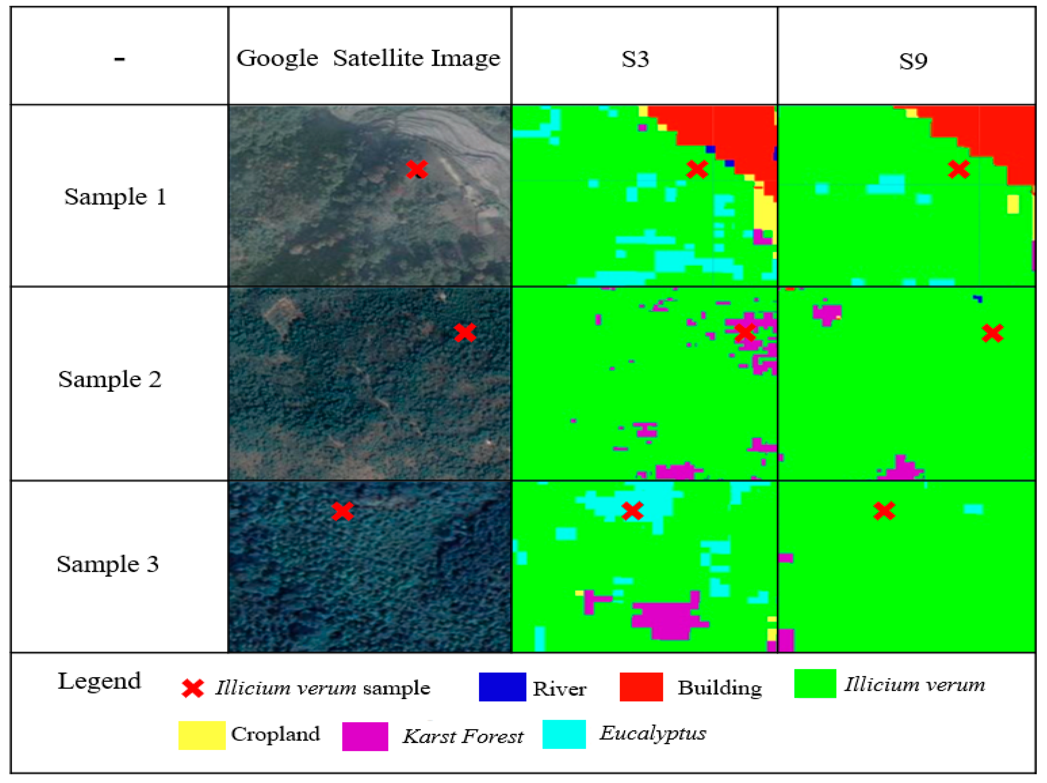
Find the best feature combination scheme to complete the extraction of Illicium verum in Leye County.

In this paper, we constructed a special feature set called the vegetation functional datasets, which were composed of the FPAR data and carbon storage data of Illicium verum in Leye County, Guangxi. Sentinel-2 data, environmental datasets, and vegetation functional datasets are combined to form an RF model to enhance the extraction of Illicium verum in Leye County, Guangxi. From another perspective, we proposed a new direction for enhancing tree species classification and validated the role of vegetation functional datasets for improving Illicium verum extraction. If functional datasets of vegetation from more tree species are obtained in the future, we can extend them to the level of multiple tree species and this approach may help to extract more information about forest species from the remote sensing data in future studies.

2. Materials and Methods

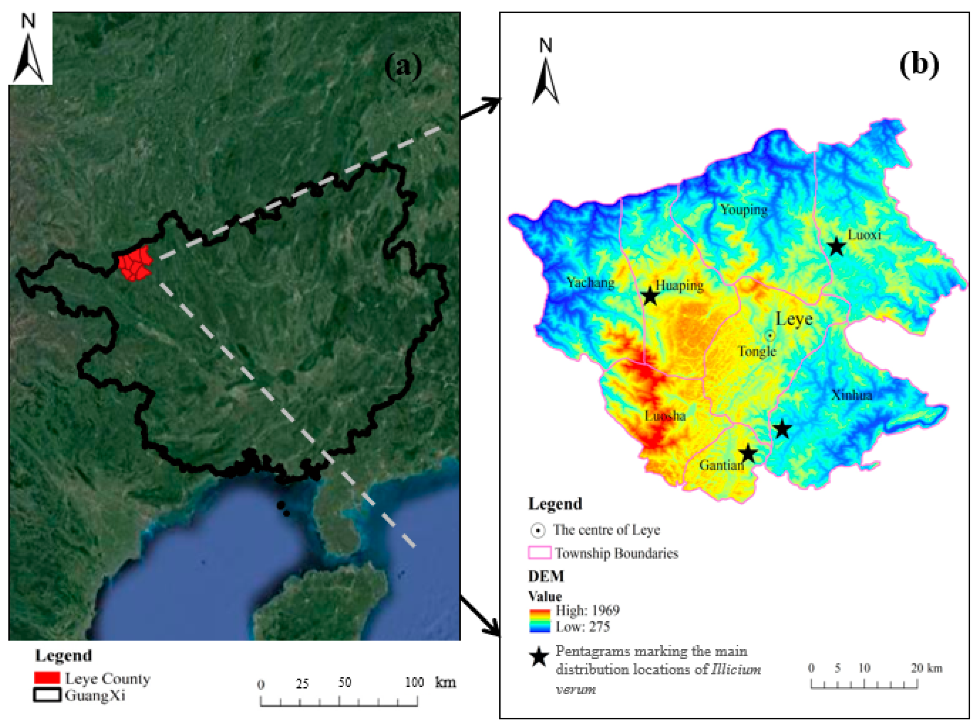
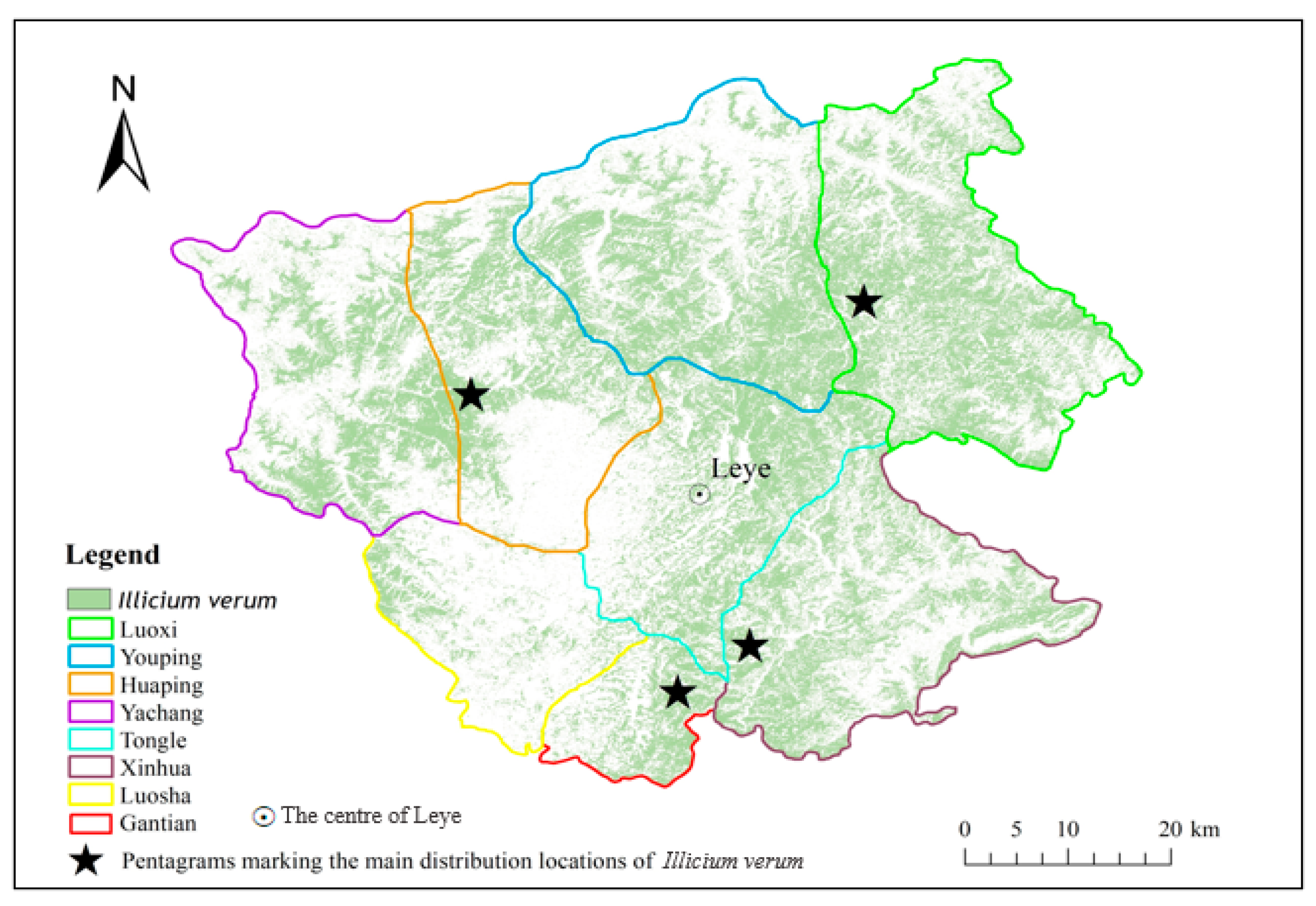
2.1. Study Area

As depicted in Figure 1a, Leye County, the study area, is in the northwest part of the Guangxi Zhuang Autonomous Region. The region is low lying in the north with an elevated terrain in the south (Figure 1b). The climate of the region is suitable for the growth of a variety of tree species.

Leye County is rich in forest resources, and its forest tree species mainly include Illicium verum, eucalyptus, and karst forest. Leye County has four townships and four towns, and the Illicium verum is mainly distributed in Luoxi, Huaping, Gantian, and Xinhua. Forty percent of Huaping is a karst forest. Xinhua has two rivers that run through the whole territory, and farmland is minly distributed on both sides of the river. Xinhua’s karst forest is in its southeast, accounting for about 12.0% of the town’s total area. Luoxi has a forest coverage rate of 80.2%. The forest coverage rate of Youping is 82.9%. Yachang is 95.0% mountainous, and suitable for a variety of crops. The town with the highest elevation in Guangxi is Tongle. Sixty-seven percent of Luoxi’s land is karst forest.

2.2. Experimental Data

2.2.1. Sentinel-1 Data and Sentinel-2 Data

The Sentinel-1 data was used in this study. The interferometric wide swath (IW) instrument mode with dual-band cross polarization (VV) and vertical transmit/horizontal receive (VH) was used. S1 data has a high spatial resolution of 10 m and a repeat cycle of 12 days. Derived from a dual-polarization C-band SAR instrument, this homogenous subset of the S1 data includes the S1 ground range detected (GRD) scenes, processed using the Sentinel-1 Toolbox to generate calibrated, orthocorrected backscatter coefficient (σ°) in decibels (dB) [19]. Alberto et al. [42] used C-band SAR backscatter to evaluate the accuracy of forest type and tree species classification and improved the tree species classification results by combining the VV and VH bands of Sentinel-1 data. Therefore, this paper introduces the dual-polarization band data of Sentinel-1 data to further improve the results of tree species classification.

The Sentinel-2 (S2) image has 13 spectral bands, including bands 2, 3, 4, and 8 having a spatial resolution of 10 m. Bands 5, 6, 7, 8A, 11, and 12 have a spatial resolution of 20 m. The spatial resolution of bands 1, 9, and 10 is 60 m. Based on previous research [43], this study selected bands 2, 3, 4, 5, 6, 7, 8, 8A, 11, and 12 (which are sensitive to tree species recognition) and resampled to 10 m spatial resolution, corrected by Sen2Cor atmospheric correction [44].

The S2A data was released on 28 March 2017, screening images with less than 20% cloud cover in the study area. At the same time, combined with the important time nodes of the tree growth period, the images from April to November were screened. Because April and June are the flowering seasons for many tree species, many trees are full of flowers in mid-July. September is the ripening period for most tree species in the study area and the leaves of the trees slowly fall from October to November. The time-series multispectral images are arranged in monthly order, providing phenological information and spectral temporal characteristics [45]. April to November of each year from 2017 to 2020 listed all S2A data that met cloud coverage requirements separately. There were 0 images in 2017 and 2018, 4 images in 2020, 5 images in 2021, and the most images in 2019 with 9 images. Therefore, this article selects 9 S2A data from April to November 2019 with less than 20% cloud cover. Next, the S2 time series images are fused into one image, and the multitype features of the S2 images are extracted to construct spectral datasets, environmental datasets, and vegetation functional datasets.

GEE provides data from over 40 years, including georeferenced and atmospheric corrected remote sensing data, where free data resources can be used for education, natural, and environmental research applications [46]. This study collected S1 and S2 data from 2019 via the GEE platform (https://earthengine.google.org/ (accessed on 23 July 2022)), covering the entire area of Leye County, Baise City, Guangxi.

2.2.2. Field Data

Field sampling data and image visual interpretation data were used as two types of ground reference data. In November 2020, samples of Illicium verum in the field in Leye County were collected (Figure 2a). The sampling standard selected the field sample plot as a square with a side length of 30 m, and the forest within 30 m around the sampling center was divided into the same tree species, and then the central forest was divided into sampling centers. Otherwise, the sample plot was abandoned and transferred to another suitable location so that the sample plot was composed of only one species [45]. Finally, the real time kinematics carrier phase difference technology was used to obtain the Illicium verum sample coordinates of the selected stand center, and the Illicium verum chest diameter and tree height data were recorded at the same time. Some of the field sampling centers for the Illicium verum were shown (Figure 3).

A total of about 1000 visually interpreted samples of six land cover types were obtained for follow-up experiments in Leye County, namely water, building, Illicium verum, karst forest, and eucalyptus, and the sample numbers of corresponding constituencies were 125, 200, 209, 201, 110, and 144, respectively. The reference data (ESRI shapefiles) was imported into GEE using the GEE Asset Management tool and determined the distribution of various types of samples in the study area using the GEE geometry tool (Figure 2b). Cross-validation of sample data for visual interpretation of images using field reference data and high spatial resolution Google Satellite images combined with texture features of different tree species. The RF and SVM classification models in GEE were used for training and the ratio of the training samples selected by the experiment to the test samples is 1:3.

2.3. Methods

In this study, a tree species classification method for enhanced extraction of Illicium verum from vegetation functional datasets was proposed. In order to explore the influence of multiple datasets on tree species classification, nine feature combination schemes were designed in this study (as shown in

Table 1. The feature subsets of various schemes.

ID of Schemes	Feature Subsets	Total Features
S1	S2 Data a + Vis b	17
S2	S2 Data + Vis + DEM c	18
S3	S2 Data + Vis + Environmental Datasets d	20
S4	S2 Data + Vis + Environmental Datasets + S1 Data e	22
S5	S2 Data + Vis + S1 Data	19
S6	S2 Data + Vis + FPAR f	18
S7	S2 Data + Vis + C f	18
S8	S2 Data + Vis + FPAR + C	19
S9	S2 Data + Vis + FPAR + C + Environmental Datasets	22

^a S2 data: Bands 2, 3, 4, 5, 6, 7, 8, 8A, 11, and 12 of Sentinel-2 data; ^b Vis: Normalized Difference Vegetation Index, Normalized Difference Water Index, Normalized Difference Built-up Index, Enhanced Vegetation Index, Ratio Vegetation Index, Normalized Difference Phenology Index and Red Edge Position Index. ^c Digital Elevation Model (DEM). ^d Environmental Datasets: DEM, slope, and aspect. ^e S1 data: VV and VH bands of Sentinel-1 data. ^f vegetation functional datasets: FPAR and carbon storage data(C).

), and the Illicium verum extraction in Leye County, Guangxi was completed by machine learning methods. The experiment mainly includes the following parts: (1) According to the S1 scheme, RF and SVM were used to compare the accuracy results of the experiment, and a fixed model was selected for the next experiment; (2) The influence of environmental datasets and S1 data on image classification was explored by using schemes S2–S5; (3) According to the schemes S6–S9, the influence of the vegetation function dataset on tree species classification was discussed, and the best feature combination scheme was found. The overall flow chart of this experiment has shown in Figure 4. S1–S9 in Figure 4 indicates the names of the nine schemes.

2.3.1. Vegetation Index Calculation

For the construction of the spectral datasets of vegetation indices, we selected the indices with high accuracy for tree species extraction: normalized difference vegetation index (NDVI), normalized difference water index (NDWI), normalized difference built-up index (NDBI), enhanced vegetation index (EVI), ratio vegetation index (RVI), normalized difference phenology index (NDPI) and red edge position index (REPI) (

Table 2. Summary table of vegetation indices selected in this experiment.

Index	Calculation	Characteristic and Reference
NDVI	$\frac{{\rho }_{NIR}-{\rho }_{RED}}{{\rho }_{NIR}+{\rho }_{RED}}$	Highly correlated with canopy leaf area index (LAI) and chlorophyll content, and used to characterize green vegetation [47].
NDWI	$\frac{{\rho }_{GREEN}-{\rho }_{NIR}}{{\rho }_{GREEN}+{\rho }_{NIR}}$	An indicator used to characterize and monitor changes in surface water content. For scattered in the mountain between the small ditch has a relatively good capture effect.
NDBI	$\frac{{\rho }_{SWIR}-{\rho }_{NIR}}{{\rho }_{SWIR}+{\rho }_{NIR}}$	To highlight the area of productive building land. NDBI is an effective index to extract urban land use information [48].
EVI	$2.5\left(\frac{{\rho }_{NIR}-{\rho }_{RED}}{{\rho }_{NIR}+6{\rho }_{RED}-7.5{\rho }_{BLUE}+1}\right)$	Helps to avoid the saturation problem of NDVI under high vegetation coverage and further reduces the influence of atmosphere and background [49].
RVI	$\frac{{\rho }_{NIR}}{{\rho }_{RED}}$	An indicator that is sensitive to high vegetation coverage area [50].
NDPI	$\frac{\left({\rho }_{NIR}-\left(0.74{\rho }_{RED}+0.26{\rho }_{swIR}\right)\right)}{\left({\rho }_{NIR}+\left(0.74{\rho }_{RED}+0.26{\rho }_{SwIR}\right)\right)}$	Helps to overcome the adverse effects of soil background heterogeneity, and has a high correlation with leaf water content due to the addition of short-wave infrared bands [51].
REPI	$705+35\left(\frac{\left({\rho }_{RED}+{\rho }_{RedEdge3}\right)∕2-{\rho }_{RedEdge1}}{{\rho }_{RedEdge2}-{\rho }_{RedEdge1}}\right)$	An indicator is sensitive to change of vegetation chlorophyll concentration, the widening of absorption characteristics due to the increase of chlorophyll concentration, and the movement of red edge to the long band direction [52].

). ρ_NIR, ρ_RED, ρ_BLUE, ρ_SWIR and ρ_RedEdgei ($i$ = 1, 2, and 3) represent the near infrared band, red band, green band, blue band, short-wave infrared band, and red edge (1, 2, and 3) band respectively.

2.3.2. Environmental Datasets

Spectral characteristics of tree species may vary geographically, making separation from other tree species using only satellite data more challenging. To account for this variability, studies often add environmental variables as auxiliary predictors to classification models [43]. Based on previous research [43], we adopted the DEM, slope, and aspect to construct the environmental datasets.

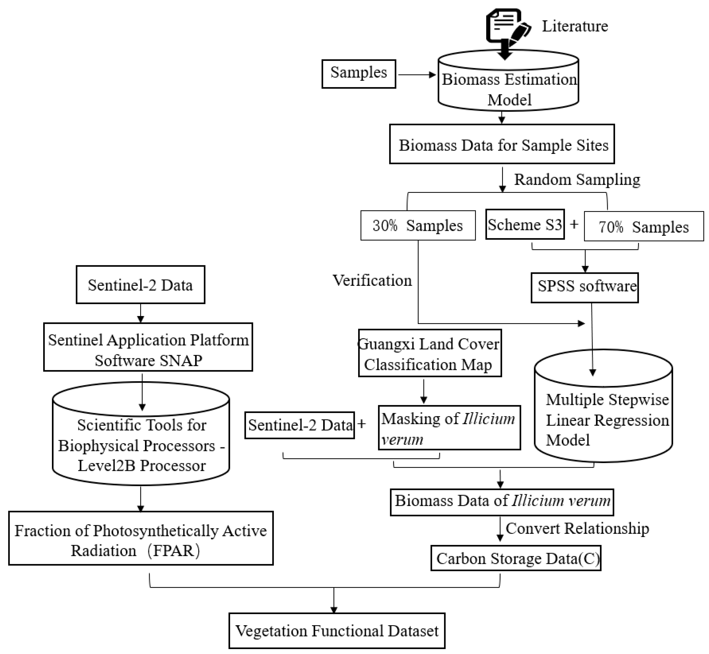
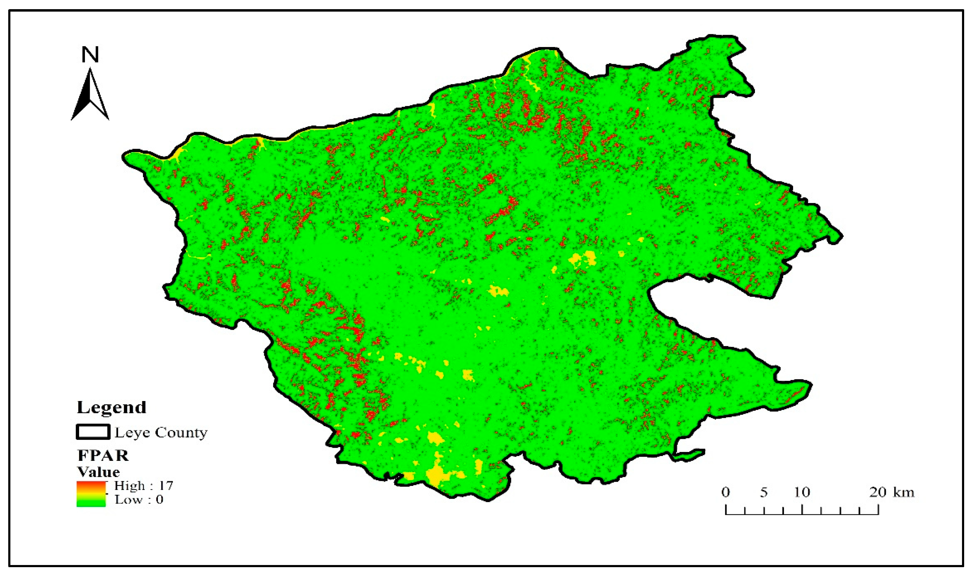
2.3.3. Vegetation Functional Datasets

This study attempts to introduce the vegetation functional datasets into the tree species extraction process. Among them, vegetation functional datasets can include FPAR, canopy chlorophyll content, carbon storage, and evapotranspiration data. However, in consideration of the accuracy and availability of the selected data, FPAR and carbon storage data were finally used as the vegetation functional datasets in this study. The detailed flow chart of vegetation functional datasets extraction is illustrated in Figure 5.

The radiation transfer model is constructed by the Sentinel application platform software biophysical processor, and the FPAR component is calculated and inverted from the S2 data to obtain the FPAR distribution in Leye County, Guangxi, as shown in Figure 6.

Based on the field survey data of Illicium verum and the biomass estimation model of Guangxi Illicium verum, the biomass of Illicium verum in the sample plot was estimated. The calculated biomass data were randomly sampled, and the biomass estimation model was established in SPSS software with 70% of the biomass data and remote sensing data. The remaining thirty percent is validation data to verify the accuracy of the model’s estimates. Then, using the remote sensing data and the biomass data obtained from the estimation model, the multiple stepwise regression model was constructed in the SPSS software. Finally, the biomass data of Illicium verum in Leye County was obtained. The estimated model of Guangxi Illicium verum biomass (Mg C/ha) in the literature is as follows [53], and D is the chest diameter of the Illicium verum.

$$W_T=0.206D^{2.277}$$

(1)

Finally, the carbon storage data of the Illicium verum in Leye County was obtained from the conversion relationship between biomass and carbon storage (Mg C/ha) [54]:

Carbon storage = biomass × 0.5

(2)

As listed in

Table 3. Summary table of carbon stock estimation models ^d.

Model	R	R2	Adjusted R2	Errors in Standard Estimates	Statistical Change
					R2 Variation	F Variation	Degrees of Freedom 1	Degrees of Freedom 2	Change in Significance F
A	0.675 a	0.456	0.452	0.12978	0.456	98.976	1	118	0.000
B	0.712 b	0.508	0.499	0.12401	0.051	12.235	1	117	0.001
C	0.726 c	0.527	0.515	0.12205	0.020	4.794	1	116	0.031

^a Predictive variables: (constant), B2; ^b Predictive variables: (constant), B2, SLOPE; ^c Predictive variables: (constant), B2, SLOPE, NDWI; ^d Dependent variable: carbon storage.

and

Table 4. Detailed parameter table of the carbon stock estimation model ^a.

Model		Unnormalized Coefficient		Normalization Coefficient	t	p-Value	Collinear Statistics
		B	stderr	Beta			Tolerance	VIF
A	constant	0.855	0.036		23.480	0.000
	B2	−0.680	0.068	−0.675	−9.949	0.000	1.000	1.000
B	constant	0.750	0.0046		16.329	0.000
	B2	−0.610	0.068	−0.606	−8.930	0.000	0.914	1.094
	SLOPE	0.226	0.065	0.237	3.498	0.001	0.914	1.094
C	constant	0.848	0.064		13.327	0.000
	B2	−0.665	0.072	−0.660	−9.266	0.000	0.803	1.246
	NDWI	−0.164	0.075	−0.155	−2.189	0.031	0.813	1.231
	SLOPE	0.251	0.065	0.264	3.886	0.000	0.885	1.129

^a Dependent variable: biomass.

, the best inversion model was model C, with a coefficient R² of 0.527, mean absolute error was 0.014399, mean absolute error was 0.024879, and root mean square error was 0.15732. Figure 7 has shown the efficacy of this fitting method. The final multiple stepwise regression model was:

Biomass = 0.848 − 0.665 × B2 + 0.251 × slope − 0.164 × NDWI

(3)

The model shows a statistically significant correlation between the biomass of Illicium verum and the B2 band, slope data, and NDWI data.

The carbon storage data of Illicium verum is shown in Figure 8. When the carbon storage data of Illicium verum was obtained, the value of other pixels was assigned the value 0, so as not to affect other categories. It was used as another component of the vegetation functional datasets.

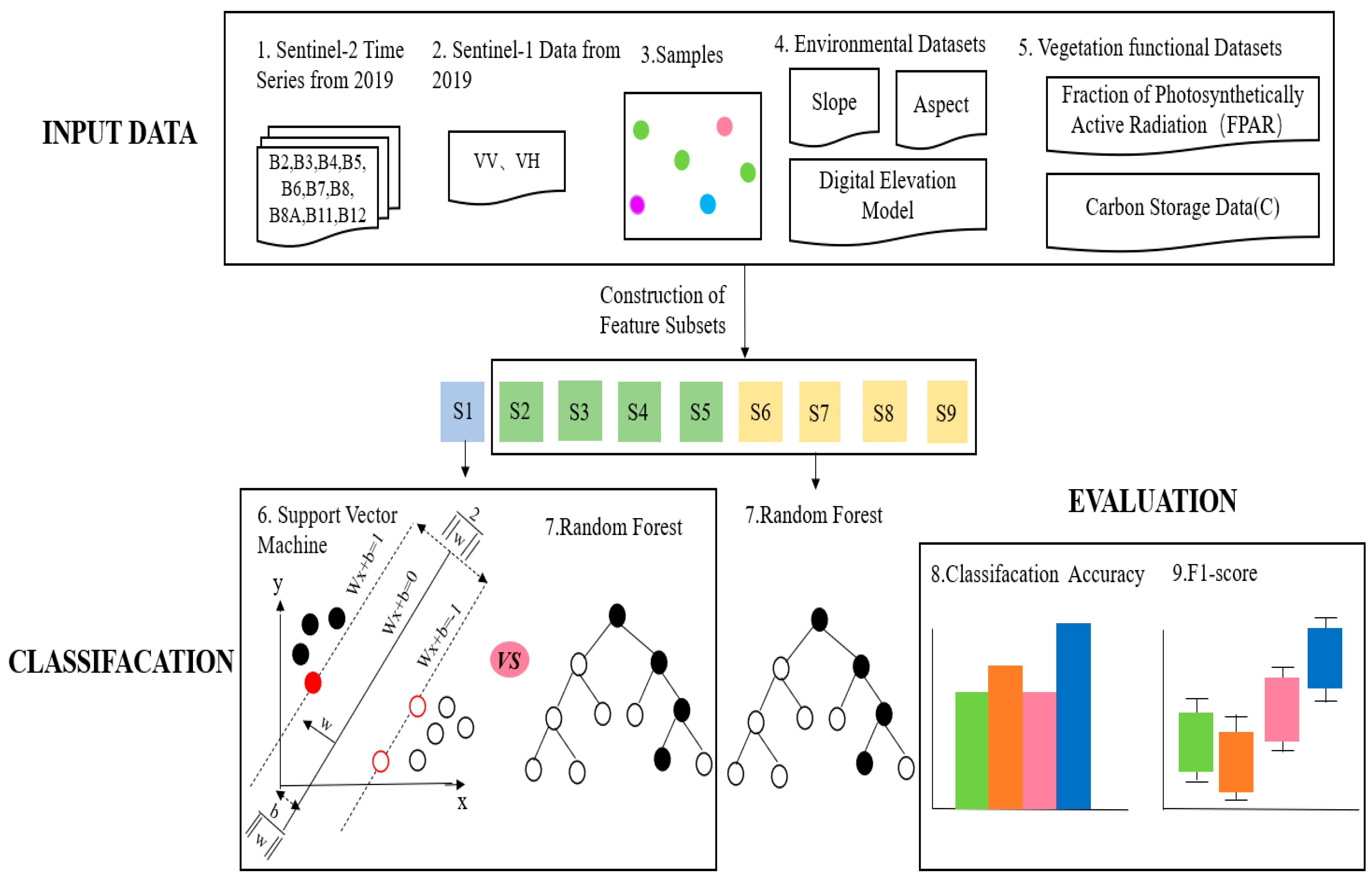
2.3.4. Random Forest Classifier and Support Vector Machine Classifier

The parameters of the RF and SVM were tested several times according to the actual situation in our study area and the final decision on each parameter was made. To make the single decision tree in RF better generalize the test data and prevent overfitting, the minimum size of the terminal node was set at 10 in GEE. In consideration of the balance between accuracy and calculation time, the number of decision trees was set to 100 in our study. SVM is a binary classification model whose basic model is a linear classifier that defines the maximum spacing in the feature space. In other words, the SVM algorithm is an optimization algorithm for solving convex quadratic programming. In this experiment, SVM parameters are set to default values. The same parameters were used in the model for different feature combinations to ensure that only the feature combinations were changing.

2.3.5. Accuracy Assessment

The quality of the experimental results used the OA and the Kappa coefficient to complete the evaluation of classification accuracy. OA is the ratio of the number of correctly classified samples to the total number of samples, and the ratio is between 0 and 1 [21]. The closer the ratio is to 1, the higher the accuracy of the classification result. TP is the positive sample correctly classified by the model; FN is the positive sample incorrectly classified by the model; FP is the negative sample incorrectly classified by the model; TN is the negative sample correctly classified by the model. The calculation formula is as follows.

$$OA=\frac{TP\times TN}{TP+FN+FP+TN}.$$

(4)

The Kappa coefficient is used to measure the agreement between the true categories and the categories predicted by the model. The higher the value of the Kappa coefficient, the higher the classification accuracy [21]. $p_0$ is the sum of the number of correctly classified samples in each category divided by the total number of samples, which is the overall classification accuracy. The calculation formula is as follows.

$$Kappa coefficient=\frac{p_0-p_e}{1-p_e}.$$

(5)

Suppose the true number of samples in each category is a1, a2, …, aC and the predicted number of samples in each category is b1, b2, …, bC. The total number of samples is n and $p_e$ is:

$$p_e=\frac{a1\times b1+a2\times b2+\cdots +ac\times bc}{n\times n}.$$

(6)

The F₁ score is a weighted average evaluation index, with a value range of [0, 1]. The closer the value is to 1, the higher the accuracy. In this study, by using different datasets to form a variety of models, the model with the better classification effect is selected. Then, the average of the F₁ score of the Illicium verum was calculated using the user accuracy (UA) and producer accuracy (PA) obtained from 10 experiments of the model. The F₁ score was used to evaluate the influence of each model on the extraction of Illicium verum. The calculation formula is as follows.

$$F_1 score=2\times \frac{PA\times UA}{PA+UA}.$$

(7)

3. Results

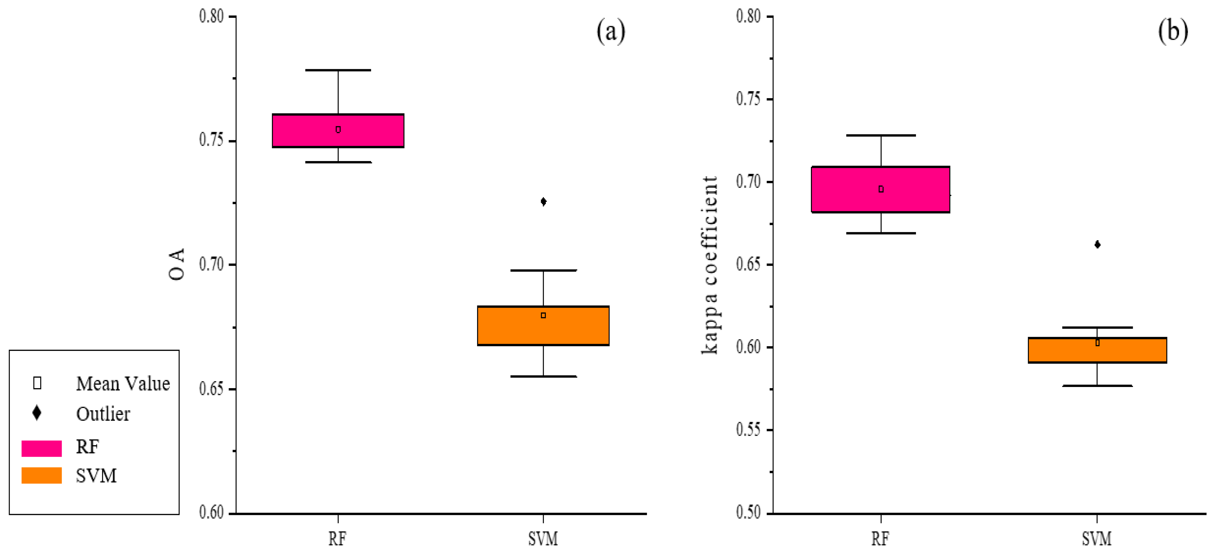
3.1. Comparison of RF and SVM Results

First, the S1 scheme, combined with the RF classifier, was used to obtain a preliminary land cover map of Leye County, Guangxi Zhuang Autonomous Region. To avoid accuracy anomalies in the classification process using RF, we did 10 replicates, with an average value of 0.7547 for OA and 0.6957 for the Kappa coefficient. At the same time, the S1 scheme was experimented with as an SVM classifier. At this point, the resulting OA was 0.6798 and the Kappa coefficient was 0.6032.

As shown in Figure 9, both from OA and Kappa coefficients, the classification accuracy of RF was greater than that of SVM. Thus, the RF classifier was used in the subsequent experiments of this study.

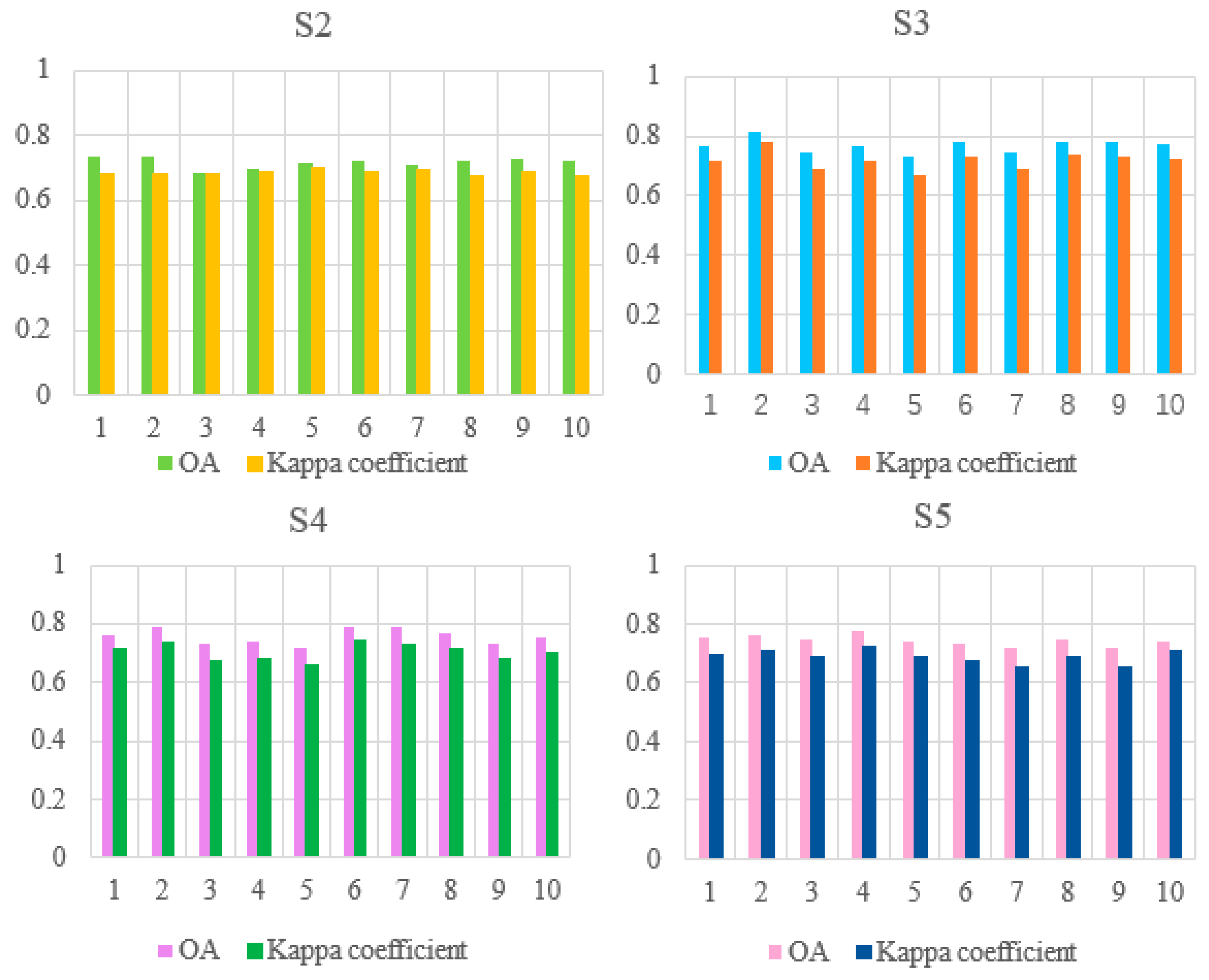
3.2. Impact of Environmental Datasets and Sentinel-1 Data on Classification Results

The RF classifier was constructed using schemes S2–S5 to complete the land cover classification of Leye County and the results obtained are shown in

Table 5. Classification Results for Schemes S2–S5.

ID of Schemes	Feature Subsets	Total Features	OA a	Kappa b
S2	S2 Data c+ VIs d+ DEM e	18	0.7368	0.6790
S3	S2 Data + VIs + Environmental Datasets f	20	0.7699	0.7190
S4	S2 Data + VIs+ Environmental Datasets +S1 Data g	22	0.7577	0.7021
S5	S2 Data + VIs + S1 Data	19	0.7434	0.6879

^a The OA value is the average of ten identical experiments. ^b The Kappa value is the average of ten identical experiments. ^c S2 Data: Bands 2, 3, 4, 5, 6, 7, 8, 8A, 11, and 12 of Sentinel-2 data; ^d VIs: Normalized Difference Vegetation Index, Normalized Difference Water Index, Normalized Difference Built-up Index, Enhanced Vegetation Index, Ratio Vegetation Index, Normalized Difference Phenology Index, and Red Edge Position Index. ^e Digital Elevation Model (DEM). ^f Environmental Datasets: DEM, slope, and aspect. ^g S1 data: VV and VH bands of Sentinel-1 data.

. Both the OA and Kappa values in the table are the average of the results obtained by RF after ten identical experiments. Among them, the highest OA and Kappa values were obtained using S3, the second highest results were obtained using S4, followed by S5, and the lowest OA and Kappa values were obtained by S2.

In ten experiments using each scheme, the OA and Kappa values are shown in Figure 10. S2–S5 means schemes 2 to 5.

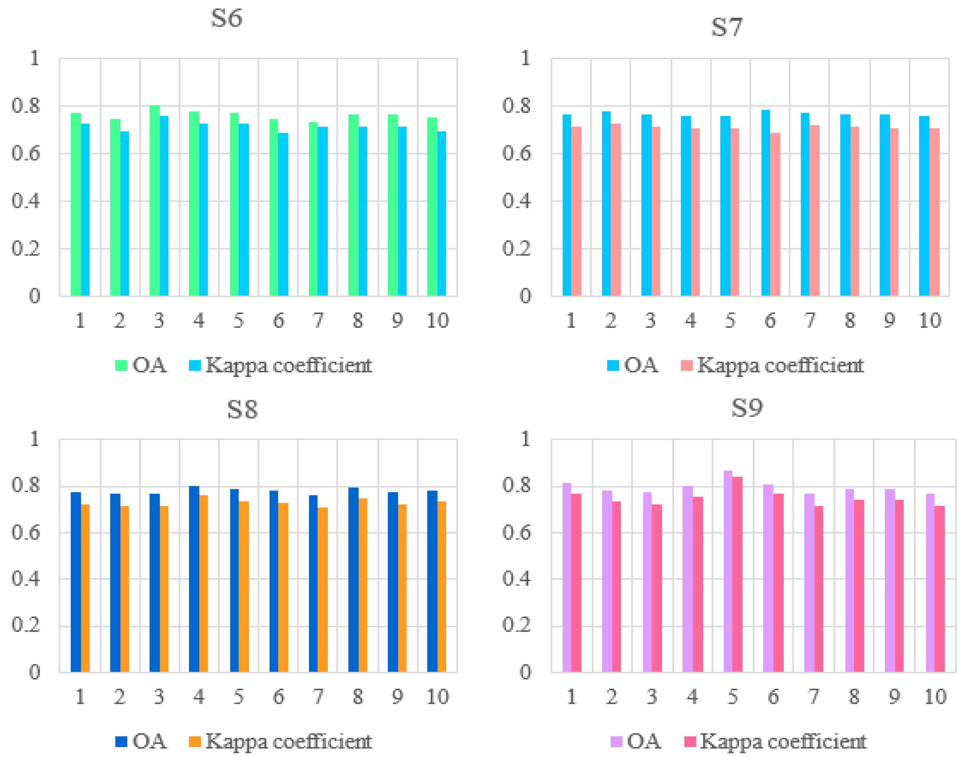
3.3. Effects of Vegetation Functional Datasets on Classification Results

The RF classifier was constructed using schemes S6–S9 to complete the land cover classification of Leye County, and the results obtained have shown in

Table 6. Classification Results for Schemes S6–S9.

ID of Schemes	Feature Subsets	Total Features	OA a	Kappa b
S6	S2 c Data + VIs d + FPAR	18	0.7651	0.7162
S7	S2 Data + VIs + C e	18	0.7676	0.7115
S8	S2 Data + Vis + FPAR +C	19	0.7774	0.7283
S9	S2 Data + VIs + FPAR + C + Environmental Dataset f	22	0.7953	0.7501

^a The OA value is the average of ten identical experiments. ^b The Kappa value is the average of ten identical experiments. ^c S2 Data: Bands 2, 3, 4, 5, 6, 7, 8, 8A, 11, and 12 of Sentinel-2 data; ^d VIs: Normalized Difference Vegetation Index, Normalized Difference Water Index, Normalized Difference Built-up Index, Enhanced Vegetation Index, Ratio Vegetation Index, Normalized Difference Phenology Index, and Red Edge Position Index. ^e C: Carbon storage data(C). ^f Environmental Datasets: DEM, slope, and aspect.

. Both the OA and Kappa values in the table were the average of the results obtained by RF after ten identical experiments. Among them, the highest OA and Kappa values were obtained using S9, the second highest results were obtained using S8, followed by S7, and the lowest OA and Kappa values were obtained by S6. The positive effects of the vegetation functional datasets in tree species classification were evidenced.

^a The OA value is the average of ten identical experiments. ^b The Kappa value is the average of ten identical experiments. ^c S2 Data: Bands 2, 3, 4, 5, 6, 7, 8, 8A, 11, and 12 of Sentinel-2 data; ^d VIs: Normalized Difference Vegetation Index, Normalized Difference Water Index, Normalized Difference Built-up Index, Enhanced Vegetation Index, Ratio Vegetation Index, Normalized Difference Phenology Index, and Red Edge Position Index. ^e C: Carbon storage data(C). ^f Environmental Datasets: DEM, slope, and aspect.

In ten experiments using each scheme, the OA and Kappa values have shown in Figure 11. S6–S9 means schemes 6 to 9.

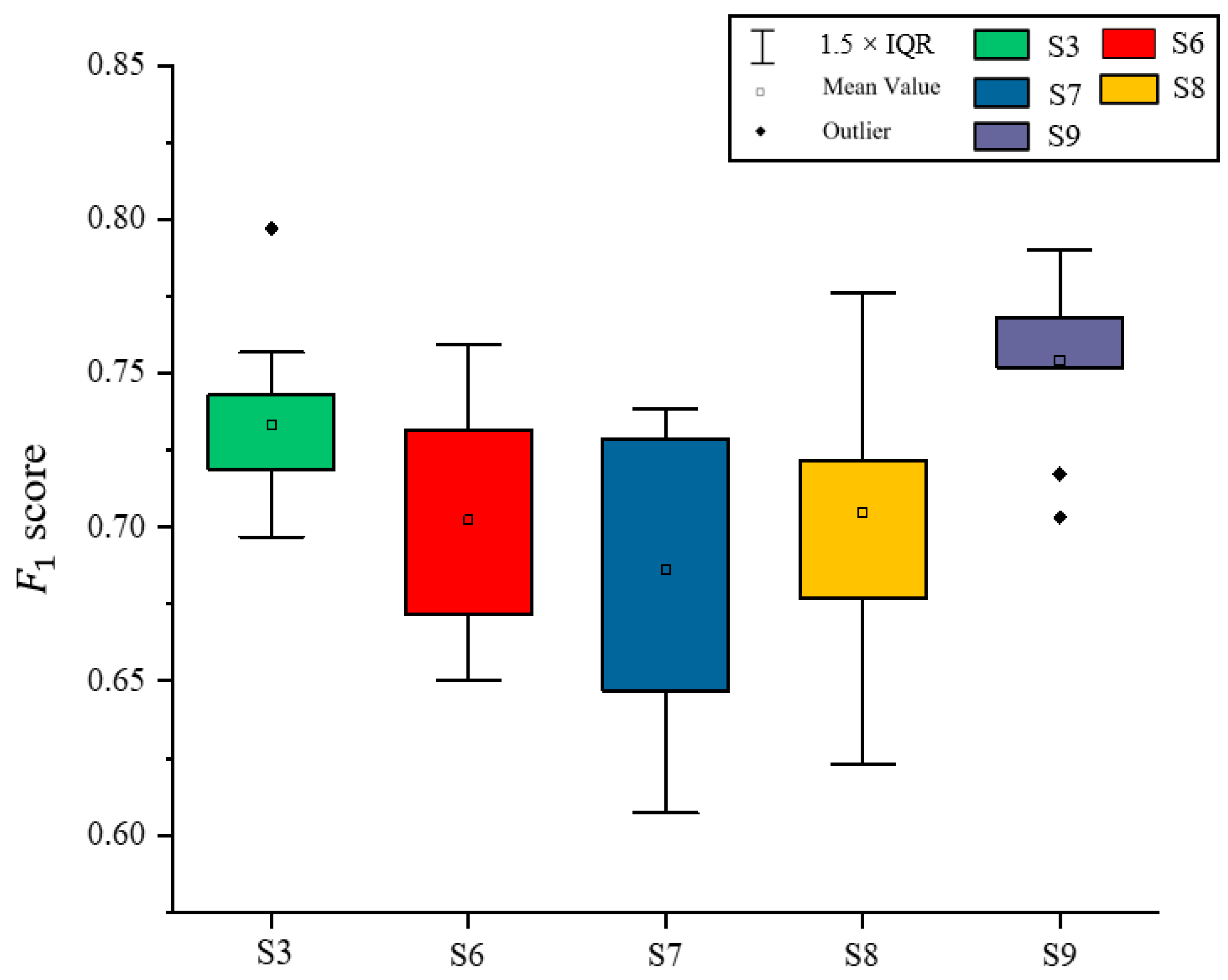
3.4. Effects of Environmental Datasets and the Vegetation Functional Datasets on Classification Results of Illicium verum

Based on the results of the experiments in Section 3.1, Section 3.2 and Section 3.3, the best classified S3 in Section 3.2 and all schemes in Section 3.3 were selected. The F₁ score on Illicium verum was calculated separately for each experiment completed by the model. As shown in Figure 12, the F₁ score was the highest when using scheme 9 to extract Illicium verum, indicating that the extraction effect of Illicium verum was the best at this time, and the highest F₁ score was 0.79.

Figure 13 has shown the distribution of the Illicium verum in Leye County extracted using S9. The positions of pentagrams in Figure 13 are consistent with the main planting distribution regions (Luoxi, Huaping, Gantian, and Xinhua) of Illicium verum in Leye County collected before the experiment.

To further explore the ability of the vegetation functional dataset for Illicium verum extraction, we selected the top two schemes for classification accuracy from the previous experiments for a detailed comparison of Illicium verum sample classification results. The details of Illicium verum extracted using S3 and S9 were compared based on the Illicium verum field survey sampling points and Google satellite imagery, as shown in Figure 14. In this case, the Google satellite images are all obtained at a scale of 1:1000.

The three sample plots in Figure 14 are from Luoxi, Huaping, and Gantian, where Illicium verum coverage is high. S3 was constructed from the S2 data, vegetation index, and environmental datasets, and S9 was constructed from the S2 data, vegetation index, environmental datasets and the vegetation functional datasets. It can be observed from Figure 14 that S9 is more robust and suited than S3 for the extraction of Illicium verum, and effectively reduce misclassification. It is further verified that the RF classification model constructed using the vegetation functional datasets positively affects the extraction of information on the Illicium verum from remote sensing data.

4. Discussion

From the experimental results in Section 3.1, RF has a higher OA and Kappa than SVM, so we know that RF performs more robustly than SVM for tree species classification in our experiments, which is consistent with the findings in most studies [21,25,26,27]. If the objects to be classified in the study area are complex, the study is prone to misclassification and omission. However, the RF classifier, with strong antioverfitting and generation abilities, is a suitable option for tree species identification and it can still give stable results even with more complex datasets [21].

There are differences in the results of each scheme for RF classification. As shown in Table 5 and Figure 10 (in Section 3.2.), the ranking of the individual schemes in terms of accuracy was S3 > S4 > S5 > S2. According to a preliminary analysis, the OA and Kappa coefficients obtained via S3 constructed with the environmental datasets were higher than those of the S2 (constructed with only one environmental variable), S4 (combined S1 data and environmental datasets), and S5 (constructed with S1 data only). At this point, S3 > S4 since the data content of S1 was in the redundant state of the experiment and cannot make more contributions to improve the classification accuracy.

S4 > S5 showed that the advantages of introducing environmental datasets for tree species classification were greater than those of the S1 data. When no environmental dataset is used, S5 > S2, which indicates that the S1 data can effectively improve the classification accuracy of tree species, however, the improvement in classification accuracy is better than that using only one environmental data. It can be seen from S3 > S2 that under the same circumstances, increasing the number of environmental datasets can more effectively improve the classification effect of tree species, and also verifies the positive effect of environmental datasets on tree species classification which is consistent with the research results of previous scholars [32].

The experiment showed that adding S1 data will cause data information redundancy and greatly reduce the classification effect. In other words, S1 data were prone to data redundancy during the classification process. Therefore, S1 data were not included in the final model construction. This is not to say that the S1 data do not promote tree species classification. On the contrary, we believe that the effect of S1 data on tree species classification needs further experimentation. As Alberto et al. [42] said, using only VH polarization images leads to higher species classification results compared to using VV or VH+VV. Therefore, in the future, we may further study the role of VV and VH bands of S1 data on tree species classification, respectively.

As can be seen from Table 6 in Section 3.3, after the introduction of vegetation functional datasets, the classification accuracy obtained using the four schemes was S9 > S8 > S7 = S6. As observed in Table 6 and Figure 11, compared with the experimental results in Section 3.1 and Section 3.2, S6 and S7 constructed RF models by introducing the vegetation functional datasets, which had positive effects on tree species extraction. There was little difference in the classification results obtained by the introduction of FPAR and carbon storage data. S8 > S6 and S7 showed that increasing the number of vegetation functional datasets can enhance the effectiveness of classification. Considering other vegetation functional datasets that have been explored by scholars [14,35,36], the next research can try to increase the number of vegetation functional datasets, such as canopy chlorophyll content and evapotranspiration data to improve the classification accuracy.

Moreover, S8 > S3 showed that the classification effect of S2 multiband data, combined with the vegetation functional datasets, was better than that of S2 multiband data combined with environmental datasets. This showed that the vegetation functional datasets were better than the environment datasets in improving the accuracy of tree species classification. From S9 > S8, we observed that adding environmental datasets to S8 can further improve the classification effect, and the improvement effect of environmental datasets and the vegetation functional datasets on classification accuracy was not suppressed by one more feature, which was different from the S1 data in Section 3.2. It indicated that the environmental datasets and the vegetation functional datasets are complementary.

S9 > S3 showed that S9 produced a better classification effect. This further indicated that increasing the vegetation functional datasets had a positive effect on the classification of tree species. In addition, compared with the combination of S2 data, environmental datasets, and S1 data, better classification results can be acquired by combining S2 data, environmental datasets, and the vegetation functional datasets. Therefore, we believe that the vegetation functional datasets have a higher positive effect on the classification of tree species.

Texture feature is also an important factor in tree species classification and plays a key role in spatial structure features. Studies have shown that the gray level co-occurrence matrix (GLCM) can effectively extract texture information [33,55]. So, in the next study, we will consider introducing texture features. As we all know, the growth cycles of different species vary. Different months in the same year show different phenological patterns. A number of studies have shown that the use of phenological characters can also improve the accuracy of tree species classification [43,46,56]. Therefore, our future studies will include phenological characteristics of Illicium verum to further improve the accuracy of classification.

As Illicium verum often exists in the form of a mixed forest, the experimental results are often accompanied by salt and pepper noise. Therefore, to further improve the classification accuracy of tree species, we propose the introduction of the object-oriented angle and LiDAR data to improve the extraction accuracy of tree species by providing multidirectional structural features. At the same time, LiDAR data can be collected at any time, regardless of the weather. LiDAR data can also be used to repair S2 data with high cloudiness, which can help us to obtain more S2 time series data and can also further increase the accuracy of the experimental results.

5. Conclusions

This study proposed a new method to enhance tree species classification and demonstrated that vegetation functional datasets can effectively improve the accuracy of Illicium verum classification. In this study, nine S2 images from 2019 were used to map six types of land cover in Leye County. Different schemes were constructed by combining different types of datasets. One of the schemes that yielded the best classification results was S9, which combined S2 multiband data with multiple vegetation indices, vegetation functional datasets, and environmental datasets. The best classification result obtained through 10 experiments was an OA of 0.8671 and a Kappa coefficient of 0.8382. The results showed that S9 containing the vegetation functional datasets had the highest Illicium verum extraction accuracy, with an F1 score of 0.79. We believe that the vegetation functional datasets can enhance the accuracy of Illicium verum classification and provide new directions for tree species identification research. If vegetation functional datasets from more tree species are obtained in the future, we can extend them to the level of multiple tree species and this approach may help to extract more information about forest species from remote sensing data in future studies.

References

1. Dalponte, M.; Bruzzone, L.; Gianelle, D. Tree species classification in the Southern Alps with very high geometrical resolution multispectral and hyperspectral data. In Proceedings of the 2011 3rd Workshop on Hyperspectral Image and Signal Processing: Evolution in Remote Sensing (WHISPERS), Lisbon, Portugal, 6–9 June 2011. [Google Scholar]
2. Waser, L.T.; Ginzler, C.; Kuechler, M.; Baltsavias, E.; Hurni, L. Semi-automatic classification of tree species in different forest ecosystems by spectral and geometric variables derived from Airborne Digital Sensor (ADS40) and RC30 data. Remote Sens. Environ. 2011, 115, 76–85. [Google Scholar] [CrossRef]
3. Schimel, D.S.; Asner, G.P.; Moorcroft, P. Observing changing ecological diversity in the Anthropocene. Front. Ecol. Environ. 2013, 11, 129–137. [Google Scholar] [CrossRef] [PubMed] [Green Version]
4. Liu, J.; Wang, X.; Wang, T. Classification of tree species and stock volume estimation in ground forest images using Deep Learning. Comput. Electron. Agric. 2019, 166, 105012. [Google Scholar] [CrossRef]
5. Turner, W.; Spector, S.; Gardiner, N.; Fladeland, M.; Sterling, E.; Steininger, M. Remote sensing for biodiversity science and conservation. Trends Ecol. Evol. 2003, 18, 306–314. [Google Scholar] [CrossRef]
6. Baldeck, C.A.; Asner, G.P.; Martin, R.E.; Anderson, C.; Knapp, D.E.; Kellner, J.R.; Joseph, W.S.; Lalit, K. Operational Tree Species Mapping in a Diverse Tropical Forest with Airborne Imaging Spectroscopy. PLoS ONE 2015, 10, e0118403. [Google Scholar] [CrossRef]
7. Ghosh, A.; Fassnacht, F.E.; Joshi, P.K.; Koch, B. A framework for mapping tree species combining hyperspectral and LiDAR data: Role of selected classifiers and sensor across three spatial scales. Int. J. Appl. Earth Obs. Geoinf. 2014, 26, 49–63. [Google Scholar] [CrossRef]
8. Piiroinen, R.; Heiskanen, J.; Maeda, E.; Viinikka, A.; Pellikka, P. Classification of Tree Species in a Diverse African Agroforestry Landscape Using Imaging Spectroscopy and Laser Scanning. Remote Sens. 2017, 9, 875. [Google Scholar] [CrossRef] [Green Version]
9. Ballanti, L.; Blesius, L.; Hines, E.; Kruse, B. Tree Species Classification Using Hyperspectral Imagery: A Comparison of Two Classifiers. Remote Sens. 2016, 8, 445. [Google Scholar] [CrossRef] [Green Version]
10. Ferreira, M.P.; Zortea, M.; Zanotta, D.C.; Shimabukuro, Y.E.; Filho, C. Mapping tree species in tropical seasonal semi-deciduous forests with hyperspectral and multispectral data. Remote Sens. Environ. 2016, 179, 66–78. [Google Scholar] [CrossRef]
11. Franklin, S.E.; Ahmed, O.S. Deciduous tree species classification using object-based analysis and machine learning with unmanned aerial vehicle multispectral data. Int. J. Remote Sens. 2018, 39, 5236–5245. [Google Scholar] [CrossRef]
12. Maschler, J.; Atzberger, C.; Immitzer, M. Individual Tree Crown Segmentation and Classification of 13 Tree Species Using Airborne Hyperspectral Data. Remote Sens. 2018, 10, 1218. [Google Scholar] [CrossRef] [Green Version]
13. Lu, D.; Weng, Q. A survey of image classification methods and techniques for improving classification performance. Int. J. Remote Sens. 2007, 28, 823–870. [Google Scholar] [CrossRef]
14. Ferreira, M.P.; Wagner, F.H.; Aragão, L.E.; Shimabukuro, Y.E.; de Souza Filho, C.R. Tree species classification in tropical forests using visible to shortwave infrared WorldView-3 images and texture analysis. ISPRS J. Photogramm. Remote Sens. 2019, 149, 119–131. [Google Scholar] [CrossRef]
15. Breiman, L. Random forests. Mach. Learn. 2001, 45, 5–32. [Google Scholar] [CrossRef] [Green Version]
16. Pal, M. Random forest classifier for remote sensing classification. Int. J. Remote Sens. 2005, 26, 217–222. [Google Scholar] [CrossRef]
17. Du, P.; Samat, A.; Waske, B.; Liu, S.; Li, Z. Random forest and rotation forest for fully polarized SAR image classification using polarimetric and spatial features. ISPRS J. Photogramm. Remote Sens. 2015, 105, 38–53. [Google Scholar] [CrossRef]
18. Belgiu, M.; Drăguţ, L. Random forest in remote sensing: A review of applications and future directions. ISPRS J. Photogramm. Remote Sens. 2016, 114, 24–31. [Google Scholar] [CrossRef]
19. You, N.; Dong, J. Examining earliest identifiable timing of crops using all available Sentinel 1/2 imagery and Google Earth Engine. ISPRS J. Photogramm. Remote Sens. 2020, 161, 109–123. [Google Scholar] [CrossRef]
20. Jafarian, Z.; Kargar, M.; Bahreini, Z. Which spatial distribution model best predicts the occurrence of dominant species in semi-arid rangeland of northern Iran? Ecol. Inform. 2019, 50, 33–42. [Google Scholar] [CrossRef]
21. Guo, Q.; Zhang, J.; Guo, S.; Ye, Z.; Deng, H.; Hou, X.; Zhang, H. Urban Tree Classification Based on Object-Oriented Approach and Random Forest Algorithm Using Unmanned Aerial Vehicle (UAV) Multispectral Imagery. Remote Sens. 2022, 14, 3885. [Google Scholar] [CrossRef]
22. Teluguntla, P.; Thenkabail, P.S.; Oliphant, A.; Xiong, J.; Gumma, M.K.; Congalton, R.G.; Yadav, K.; Huete, A. A 30-m landsat-derived cropland extent product of Australia and China using random forest machine learning algorithm on Google Earth Engine cloud computing platform. ISPRS J. Photogramm. Remote Sens. 2018, 144, 325–340. [Google Scholar] [CrossRef]
23. Azzari, G.; Lobell, D. Landsat-based classification in the cloud: An opportunity for a paradigm shift in land cover monitoring. Remote Sens. Environ. 2017, 202, 64–74. [Google Scholar] [CrossRef]
24. Zhang, X.; Wu, B.; Ponce-Campos, G.E.; Zhang, M.; Chang, S.; Tian, F. Mapping up-to-date paddy rice extent at 10 m resolution in china through the integration of optical and synthetic aperture radar images. Remote Sens. 2018, 10, 1200. [Google Scholar] [CrossRef] [Green Version]
25. Qin, H.; Zhou, W.; Yao, Y.; Wang, W. Individual tree segmentation and tree species classification in subtropical broadleaf forests using UAV-based LiDAR, hyperspectral, and ultrahigh-resolution RGB data. Remote Sens. Environ. 2022, 280, 113143. [Google Scholar] [CrossRef]
26. Plakman, V.; Janssen, T.; Brouwer, N.; Veraverbeke, S. Mapping species at an individual-tree scale in a temperate Forest, using Sentinel-2 images, airborne laser scanning data, and random Forest classification. Remote Sens. 2020, 12, 3710. [Google Scholar] [CrossRef]
27. Raczko, E.; Zagajewski, B. Comparison of support vector machine, random forest and neural network classifiers for tree species classification on airborne hyperspectral APEX images. Eur. J. Remote Sens. 2017, 50, 144–154. [Google Scholar] [CrossRef] [Green Version]
28. Zhang, B.; Zhao, L.; Zhang, X. Three-dimensional convolutional neural network model for tree species classification using airborne hyperspectral images. Remote Sens. Environ. 2020, 247, 111938. [Google Scholar] [CrossRef]
29. Axelsson, A.; Lindberg, E.; Reese, H.; Olsson, H. Tree species classification using Sentinel-2 imagery and Bayesian inference. Int. J. Appl. Earth Obs. Geoinf. 2021, 100, 102318. [Google Scholar] [CrossRef]
30. Wang, K.; Wang, T.; Liu, X. A Review: Individual Tree Species Classification Using Integrated Airborne LiDAR and Optical Imagery with a Focus on the Urban Environment. Forests 2019, 10, 1. [Google Scholar] [CrossRef] [Green Version]
31. Lechner, M.; Dostálová, A.; Hollaus, M.; Atzberger, C.; Immitzer, M. Combination of Sentinel-1 and Sentinel-2 Data for Tree Species Classification in a Central European Biosphere Reserve. Remote Sens. 2022, 14, 2687. [Google Scholar] [CrossRef]
32. Ewa, G.; David, F.; Katarzyna, O. Evaluation of machine learning algorithms for forest stand species mapping using Sentinel-2 imagery and environmental data in the Polish Carpathians. Remote Sens. Environ. 2020, 251, 7. [Google Scholar]
33. Deur, M.; Gašparović, M.; Balenović, I. Tree species classification in mixed deciduous forests using very high spatial resolution satellite imagery and machine learning methods. Remote Sens. 2020, 12, 3926. [Google Scholar] [CrossRef]
34. Götze, C.; Gerstmann, H.; Gläßer, C.; Jung, A. An approach for the classification of pioneer vegetation based on species-specific phenological patterns using laboratory spectrometric measurements. Phys. Geogr. 2017, 38, 524–540. [Google Scholar] [CrossRef]
35. Violle, C.; Navas, M.L.; Vile, D.; Kazakou, E.; Fortunel, C.; Hummel, I.; Garnier, E. Let the concept of trait be functional! Oikos 2007, 116, 882–892. [Google Scholar] [CrossRef]
36. Violle, C.; Reich, P.B.; Pacala, S.W.; Enquist, B.J.; Kattge, J. The emergence and promise of functional biogeography. Proc. Natl. Acad. Sci. USA 2014, 111, 13690–13696. [Google Scholar] [CrossRef] [PubMed] [Green Version]
37. Zhu, J.; Huang, Z.; Sun, H.; Wang, G. Mapping Forest Ecosystem Biomass Density for Xiangjiang River Basin by Combining Plot and Remote Sensing Data and Comparing Spatial Extrapolation Methods. Remote Sens. 2017, 9, 241. [Google Scholar] [CrossRef] [Green Version]
38. Bilous, A.; Myroniuk, V.; Holiaka, D.; Bilous, S.; See, L.; Schepaschenko, D. Mapping growing stock volume and forest live biomass: A case study of the Polissya region of Ukraine. Environ. Res. Lett. 2017, 12, 105001. [Google Scholar] [CrossRef] [Green Version]
39. Wang, Z.; Ma, Y.; Chen, P.; Yang, Y.; Fu, H.; Yang, F.; Raza, M.A.; Guo, C.; Shu, C.; Sun, Y.; et al. Estimation of Rice Aboveground Biomass by Combining Canopy Spectral Reflectance and Unmanned Aerial Vehicle-Based Red Green Blue Imagery Data. Front. Plant Sci. 2022, 13, 903643. [Google Scholar] [CrossRef]
40. Santi, E.; Paloscia, S.; Pettinato, S.; Fontanelli, G.; Mura, M.; Zolli, C.; Maselli, F.; Chiesi, M.; Bottai, L.; Chirici, G. The potential of multifrequency SAR images for estimating forest biomass in Mediterranean areas. Remote Sens. Environ. 2017, 200, 63–73. [Google Scholar] [CrossRef]
41. Hongwei, M.; Hai, L.; Shunbin, Y.; Wei, Z. Analysis and Prospect on the Application of Tree Species Classification Based on Forestry Remote Sensing. For. Resour. Manag. 2020, 3, 118. [Google Scholar] [CrossRef]
42. Udali, A.; Lingua, E.; Persson, H.J. Assessing Forest Type and Tree Species Classification Using Sentinel-1 C-Band SAR Data in Southern Sweden. Remote Sens. 2021, 13, 3237. [Google Scholar] [CrossRef]
43. Hemmerling, J.; Pflugmacher, D.; Hostert, P. Mapping temperate forest tree species using dense Sentinel-2 time series. Remote Sens. Environ. 2021, 267, 112743. [Google Scholar] [CrossRef]
44. Louis, J.; Debaecker, V.; Pflug, B.; Main-Knorn, M.; Gascon, F. SENTINEL-2 SEN2COR: L2A Processor for Users. In Proceedings of the Living Planet Symposium, Prague, Czech Republic, 9–13 May 2016. [Google Scholar]
45. Wan, H.; Tang, Y.; Jing, L.; Li, H.; Qiu, F.; Wu, W. Tree species classification of forest stands using multisource remote sensing data. Remote Sens. 2021, 13, 144. [Google Scholar] [CrossRef]
46. Venkatappa, M.; Sasaki, N.; Anantsuksomsri, S.; Smith, B. Applications of the Google Earth Engine and Phenology-Based Threshold Classification Method for Mapping Forest Cover and Carbon Stock Changes in Siem Reap Province, Cambodia. Remote Sens. 2020, 12, 3110. [Google Scholar] [CrossRef]
47. Han, Y.; Meng, J.; Xu, J. Soybean growth assessment method based on NDVI and phenological calibration. Trans. Chin. Soc. Agric. Eng. 2017, 33, 177–182. [Google Scholar] [CrossRef]
48. Madhusudhan, M.; Ambujam, N.K. An urban ecology approach to land-cover changes in the Adyar sub-basin: Comparative analysis of NDWI, NDVI and NDBI using remote sensing. Int. J. Environ. Sustain. Dev. 2021, 1, 1. [Google Scholar] [CrossRef]
49. Panigrahi, S.; Verma, K.; Tripathi, P. Review of MODIS EVI and NDVI Data for Data Mining Applications. In Data Deduplication Approaches: Concepts, Strategies, and Challenges; Academic Press: Cambridge, MA, USA, 2021; pp. 231–253. [Google Scholar] [CrossRef]
50. Zefeng, X.; Ying, L.; Rongxin, D.; Honglei, Z.; Bolin, F. Extracting Farmland Shelterbelt Automatically Based on ZY-3 Remote Sensing Images. Sci. Silvae Sin. 2016, 52, 11–20. [Google Scholar] [CrossRef]
51. Xu, D.; Wang, C.; Chen, J.; Shen, M.; Shen, B.; Yan, R.; Li, Z.; Karnieli, A.; Chen, J.; Yan, Y. The superiority of the normalized difference phenology index (NDPI) for estimating grassland aboveground fresh biomass. Remote Sens. Environ. 2021, 264, 112578. [Google Scholar] [CrossRef]
52. Qian, B.; Huang, W.; Ye, H. Inversion of winter wheat chlorophyll contents based on improved algorithms for red edge position. Nongye Gongcheng Xuebao/Trans. Chin. Soc. Agric. Eng. 2021, 36, 162–170. [Google Scholar] [CrossRef]
53. Zhenchuan, W.; Hu, D.; Tongqing, S.; Wanxia, P.; Fuping, Z.; Zhaoxia, Z.; Hao, Z. Allometric models of major tree species and forest biomass in Guangxi. Acta Ecol. Sin. 2015, 35, 4462–4472. [Google Scholar]
54. Jingyun, F.; Anping, C. Dynamic forest biomass carbon pools in China and their significance. Acta Bot. Sin. 2001, 43, 967–973. [Google Scholar]
55. Lin, X.; Peng, D.L.; Huang, G.S.; Wang, X.J. Object-oriented classification with multi-scale texture feature based on remote sensing image. Eng. Surv. Mapp. 2016, 25, 22–27. [Google Scholar] [CrossRef]
56. Valderrama-Landeros, L.; Flores-Verdugo, F.; Rodríguez-Sobreyra, R.; Kovacs, J.M.; Flores-de-Santiago, F. Extrapolating canopy phenology information using Sentinel-2 data and the Google Earth Engine platform to identify the optimal dates for remotely sensed image acquisition of semiarid mangroves. J. Environ. Manag. 2021, 279, 111617. [Google Scholar] [CrossRef] [PubMed]
Figure 1. Study area location distribution map: (a) Location map of Leye County, Guangxi using Google satellite imagery; (b) Digital Elevation Model of Leye County. Pentagrams were used to highlight the four areas in the study area with the largest area covered by Illicium verum, namely Luoxi, Huaping, Gantian, and Xinhua.
Remotesensing 14 06248 g001
Figure 2. (a) Distribution map of Illicium verum samples from field surveys (b) Distribution map of six types of land cover samples.
Remotesensing 14 06248 g002
Figure 3. Location map of sampling center of partial field Illicium verum.
Remotesensing 14 06248 g003
Figure 4. Flow chart of the overall experiment.
Remotesensing 14 06248 g004
Figure 5. Flowchart for building vegetation functional datasets.
Remotesensing 14 06248 g005
Figure 6. Distribution map of FPAR.
Remotesensing 14 06248 g006
Figure 7. Normal P-P plots of regression normalized residuals.
Remotesensing 14 06248 g007
Figure 8. Carbon storage (Mg C/ha) distribution map of Illicium verum in Leye County.
Remotesensing 14 06248 g008
Figure 9. Comparison of classification results of RF and SVM: (a) The OA comparison chart of the two models; (b) Kappa coefficient comparison chart of the two models.
Remotesensing 14 06248 g009
Figure 10. Map of OA and Kappa values for the performance of the models assembled from schemes 2 to 5 in ten experiments.
Remotesensing 14 06248 g010
Figure 11. Map of OA and Kappa values for the performance of the models assembled from schemes 6 to 9 in ten experiments.
Remotesensing 14 06248 g011
Figure 12. Comparative map of F1 score of Illicium verum extracted using different schemes.
Remotesensing 14 06248 g012
Figure 13. Distribution of Illicium verum in Leye County.
Remotesensing 14 06248 g013
Figure 14. Comparison of Illicium verum extraction details between S3 and S9 with Google Satellite Image.
Remotesensing 14 06248 g014