Abstract
The results of modernization of a mobile lidar for the airborne monitoring of the methane content in the atmosphere are presented. The modernization was carried out on the basis of in situ tests, several engineering solutions, and preliminary numerical simulations. The in situ tests showed a possibility of sounding background tropospheric methane concentrations along a 500 m surface path. During the modernization, the airborne lidar for methane monitoring was supplemented with an off-axis mirror collimator, which made it possible to reduce the divergence of laser radiation by a factor of 4. The overlapping function was simulated for a biaxial scheme of the mobile lidar with radii of the light-sensitive zone of the receiving optics of 0.1, 0.3, 0.5, 0.8 and 1 mm. The dimensions of the light-sensitive zone were found to provide complete coverage of the field of view of the telescope and a laser beam; the length of the “dead” zone was estimated when a laser beam propagated parallel to the optical axis of the telescope. Airborne methane monitoring in the atmosphere in the informative wavelength range (2916.55–2917 cm−1 on-line and 2915.00 cm−1 off-line) was numerically simulated for midlatitude and Arctic summer. Thus, on the basis of the work carried out, the design of the mobile airborne lidar is substantiated, which is to operate as a part of the Tu-134 “Optik” aircraft laboratory of IAO SB RAS and to perform methane monitoring vertically downwards. The airborne lidar was tested during test flights and the Arctic expedition in 2022. The first experimental results of lidar measurements of the averaged methane concentration vertically downwards from sounding altitudes of 2000–3000, 380, and 270 m were obtained for mid-latitude summer and Arctic summer.
1. Introduction
Methane (CH4) is one of the key organic substances in the atmosphere. The monitoring of its atmospheric concentrations and altitude distribution is increasing in importance because of its strong effect on the Earth’s climate [1]. The scientific problem of methane detection and monitoring of its content in the atmosphere, using spectroscopic techniques and sounding tools, is important in the context of knowledge about anthropogenic and natural factors of an increase in the total content of greenhouse gases on the planet, and their contribution to climate change. Mobile lidar systems capable of performing integral and spatially distributed methane measurements are essential to ensure operational environmental monitoring in remote regions where there is no measuring infrastructure.
There are four main methane absorption bands: near 1.65, 2.3, 3.3–3.4, and 7.7 µm [2]. The methane absorption bands near 1.65 and 3.3 µm are commonly used for laser remote sensing of methane, and sounding techniques are the most developed in these wavelength ranges. The airborne IPDA (Integrated-Path Differential Absorption) lidar [3], sTDLAS (Standoff Tunable Diode Laser Absorption Spectroscopy) system [4], ALMA (aerial laser methane assessment) system [5], and IPDA CHARM-F (CO2 and CH4 Remote Monitoring—Flugzeug) lidar [6] operate at the wavelength λ = 1.65 μm; the compact mid-infrared DIfferential Absorption Lidar (DIAL) [7], Airborne Natural Gas Emission Lidar (ANGEL) system [8], and CHARM—a helicopter-borne lidar system [9]—operate at the wavelengths λ = 3.3–3.4 µm.
At present, ground-based IPDA and DIAL laser systems for methane monitoring are well developed. For example, the design of a photodetector for a DIAL/IPDA system, which was used to measure CH4 at a wavelength of 1646 nm at distances from 3 to 9 km, has been reported [10]. A ground-based IPDA system was designed for night-time monitoring of H2O, CO2, and CH4; it operated in the wavelength range 1.60–1.65 μm (the working methane monitoring wavelength is 1645 nm); the methane sensing range is 2.75 km [11]. Using IPDA lidar, the concentration of methane with detection limits of 595 ppb·m is in the 3.1–3.5 μm spectral range at distances of 70 m [12]. Methane with detection limits of 50 ppb was measured in the 3.3–3.4 μm range at distances of 1 km from a mobile DIAL platform [13]. In the National Physical Laboratory (UK), sensors for atmospheric monitoring (in particular, greenhouse gases and volatile organic compounds) have been developed [14].
Additionally, airborne CH4 monitoring systems based on lasers with OPO in the near and mid-IR spectral regions have been developed. Measurements of the total methane content in the atmosphere in the 3–11 km altitude range using an onboard pulsed IPDA system were taken [15]. Based on the first experiments [15], the IPDA system was upgraded and described in [16]. The design of an airborne IPDA system for methane and carbon dioxide vertical profiling was developed [17]. This system is mounted onboard the German research aircraft laboratory HALO (High Altitude Lidar Observatory). Later on, that system was called CHARM-F (CO2 and CH4 Remote Monitoring—Flugzeug) [6]. A CoMet expedition (simultaneous measurements of CO2 and CH4 using an airborne IPDA system) was carried out [18]. In 2018, the CoMet 1.0 mission was carried out with research flights; it was focused on measuring greenhouse gases (CO2 and CH4) over Europe [19]. In particular, the flights took place over one of the most powerful sources of methane in the European Union—the Upper Silesian coal basin (southern Poland), where methane emissions from coal ventilation shafts were assessed [20,21,22]. In general, this project is aimed at the validation of greenhouse gas satellite measurements (such as Sentinel 5-P, GOSAT-2, and MERLIN [23,24,25]) and the development of new combined active and passive remote sensing techniques for measuring greenhouse gases from space. Additionally, using the HALO aircraft, IPDA-DIAL methane measurements has been implemented for the first time [26].
Thus, we can conclude that the study of greenhouse gases (in particular, methane) with the use of airborne equipment is extremely urgent, particularly due to the full coverage of tropospheric altitudes in experiments and applicability in hard-to-reach areas, but for the presented systems [15,16,17,18,19,20,21,22], access to the Russian sector of the Arctic is limited.
A stationary IR lidar has been designed at the Institute of Atmospheric Optics, Siberian Branch, Russian Academy of Sciences (IOA SB RAS), and upgraded to study the gas composition (in particular, methane) of the atmosphere. The results [27,28] made it possible to formulate the concept of a mobile IR lidar for monitoring methane and, subsequently, to develop an experimental prototype of a ground-based mobile IR lidar for monitoring methane along horizontal tropospheric paths [29].
The experience we gained during studies [27,28,29] made it possible to suggest engineering solutions, to upgrade the ground-based mobile methane monitoring lidar system, and to configure the airborne methane monitoring lidar system for vertical downward sensing.
This paper presents the modeling calculations of methane monitoring in the troposphere along a vertical downward aircraft board and the calculation of the lidar overlap function of the airborne lidar. Additionally, we present the results of the development and testing of a ground-based lidar for methane monitoring in the midlatitude summer and its modernization for airborne conditions on a Tu-134 “Optic” aircraft laboratory of the IAO SB RAS. The results of the experimental approbation of the airborne lidar for the conditions in the mid-latitude summer and Arctic summer are given.
Installation of the lidar system on the Tu-134 “Optik” aircraft laboratory of IAO SB RAS and its testing during flight expeditions in conditions of midlatitude summer and Arctic summer, along the route passing through the Vasyugan swamps and the Russian sector of the Arctic, will provide unique information for the lidar community on the study of methane content in the atmosphere.
2. Materials and Methods
2.1. Differential Absorption Method
To isolate the contribution of the absorption of individual atmospheric gases to the laser beam attenuation, the differential absorption method is usually used [30,31,32,33,34]. The differential absorption and scattering method consists of the use of two laser lines: near the center of the absorption line of a gas under study (on resonance, on-line) and in the wing of the absorption line (off resonance, off-line). Laser radiation undergoes molecular and aerosol absorption and scattering while propagating through the atmosphere. At the wavelengths specified, the radiation is absorbed with different intensities due to molecular absorption. To eliminate the aerosol attenuation effect, the laser lines are specified at the minimum possible space between each other, maintaining a possibility of resolving the difference in lidar signals due to molecular absorption. As a result, the concentrations of gases along sounding paths can be retrieved from the ratio of lidar signals.
In the differential absorption method, molecules and atmospheric aerosol are used as a distributed reflector, which allows the remote profiling of gas impurities with a spatial resolution of n × ΔR (ΔR = cτ/2, where c-speed of light = 3 × 10⁸ m/s, τ is the laser pulse duration 10 ns, and n > 2). Lidars based on this technique are called range-resolved DIfferential Absorption Lidars (DIALs). When implementing the path differential absorption technique (IPDA), a signal reflected or diffusely reflected from different topographic objects is recorded; special mirror reflectors or natural topographic objects (trees, buildings, and the Earth’s surface) can serve as topographic targets. This method allows for the estimation of the path-average gas concentrations in certain directions which correspond to the azimuth of topographic targets with high sensitivity. The gas concentration accuracy depends on the following parameters:
- -
- Lidar signal recording error;
- -
- Errors in gas absorption cross-section found experimentally or from HITRAN [35];
- -
- Information content of selected wavelength pairs inside (λon) and outside (λoff) an absorption line, for which a large differential absorption cross section , narrow spectral range Δλ = λon − λoff, and a few interfering gases are desirable;
- -
- Detector parameters (sensitivity).
Differential absorption sounding of trace atmospheric gases is based on the effect of resonance absorption of laser radiation within a selective absorption line of a gas under study. The gas concentration averaged over the spatial range ΔR is defined in this case by the equation [30]:
where and are the absorption cross-sections along a sounding path at the point R at frequencies inside (νon) and outside(νoff) the profile of the selective absorption line of the gas under study, which are preliminary calculated with the use of model altitude profiles of the meteo parameters P(νon, R), P(νoff, R), P(νon, R + ΔR), and P(νoff, R + ΔR) are the laser echo signals at the sounding frequencies νon and νoff from the points R and R + ΔR along the sounding path recorded by the lidar receiver.
The lidar signals are described with the laser ranging equation; in the single scattering approximation, it can be written as [30]:
where χ is the transmittance of the receiving optics of the lidar; P0 is the power of laser radiation sent from the lidar point R0; c is the speed of light; τ is the laser pulse duration; A0 is the effective area of the receiving optics; and are the volume coefficients of molecular and aerosol backscattering of laser radiation; and α(ν,R) is the profile of the radiation attenuation coefficient.
The path-average concentration can be obtained using the equation [36,37]:
where Δτg is the differential optical depth of a gas under study, L is the path length, Δki is the differential absorption coefficient of a gas, Pon and Poff are laser echo signals at the sensing frequencies νon and νoff, Eon and Eoff are the initial laser pulse energies, ρon and ρoff are the target albedos, and θA = Δτint + ΔτΣ are the differential optical depths that are caused by aerosol extinction and the absorption by other gases.
2.2. Theory of Lidar Overlap Function
For the correct interpretation of lidar sensing data, it is necessary to take into account all factors which can affect the final results of the retrieval of parameters under study. Therefore, during this work, we numerically simulated lidar sensing of methane in the troposphere. In particular, the lidar overlap function was calculated to determine additional requirements for the parameters of the receiving part.
Any lidar which is created to solve a specific problem should meet certain requirements; therefore, the choice of the transceiver geometry and estimation of its potential capabilities is an important step in designing works [38]. Let us consider the biaxial scheme of the lidar transceiver which is often used in practice (Figure 1).
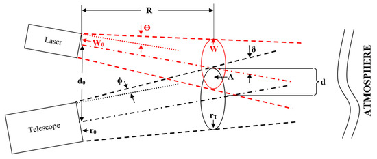
Figure 1.
Biaxial scheme of lidar, which shows the condition for partial overlap between the telescope field-of-view and a laser beam ( is the telescope radius; is the laser beam radius; is the distance between the laser beam and telescope centers; θ is the radiation divergence half-angle; rT is radius of the field of view of the optical receiving system in the plane of the object under study; W is radius of the laser pulse in the plane of the object under study; d is distance on the plane of the object under study between the points of intersection with the plane of the laser and telescope axes; and is half the divergence angle of the optical receiving system).
When radiation propagates through the atmosphere and lidar signals are recorded following this scheme, three cases are possible [39]:
The axes of the telescope and the laser in a lidar are spaced far apart, as the field of view of the receiving optics does not overlap the area illuminated by the laser in the plane of an object under study (Figure 2a), i.e., , if .
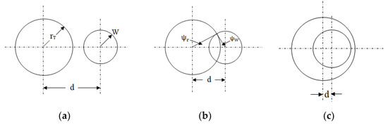
Figure 2.
Three cases of overlapping between the telescope field-of-view and a laser beam for a biaxial lidar: (a) no overlap; (b) partial overlapping; (c) complete overlapping (rT is the radius of the circular field of view; W is the radius of the circular region of laser illumination).
The distance between the axes of the telescope and the laser in a lidar is sufficiently small, so the area illuminated by the laser on the plane of an object under study completely or partially falls in the field-of-view of the receiving system (Figure 2c), i.e., if , then (the smaller of and ).
The distance between the axes of the telescope and laser in a lidar are within the range (Figure 2b from [39]).
Under these conditions, introducing dimensionless parameters [39]:
Assuming a homogeneous intensity distribution over the illumination area in the range R and taking into account the biaxial receiving system with the space d between the laser and the telescope optical axes, the geometrical factor can be considered a simple overlap function and written as [39,40]:
The overlap coefficient depends on the normalized length z, angular parameters θ, ϕ, and δ, and scale parameters A and D.
2.3. Ground-Based Mobile Lidar System
The first in situ tests of the mobile IR lidar for methane monitoring along surface horizontal paths were carried out in May–June 2021 [41]. The mobile lidar included an IR OPO laser system, Cassegrain telescope, photodetector (PD) VIGO, analog-to-digital converter (ADC) and personal computer (PC). The informative wavelengths (3428.428 nm on-line and 3431.708 nm off-line) were preliminarily found in the numerical simulation for the lidar and midlatitude summer conditions (the midlatitude summer model corresponds to the geographic coordinates and season of in situ measurements at the Fonovaya observatory of IAO SB RAS (Tomsk region) [42]). The lidar was also equipped with an alignment red laser (630 nm) coaxial with the on- and off-wavelengths of methane monitoring. The output pulse energy was ≤4.5 mJ at on- and off-line and the laser linewidth was ≤1.5 cm−1.
The optical scheme of the experiments and the lidar assembled and mounted at the experimental site are shown in Figure 3. At 50 m from the point of the experiment, there is a stationary post [42] for measuring various meteorological parameters of the atmosphere, including the Picarro gas analyzer. For checking the alignment of red (630 nm) and IR beams (3428.428 nm and 3431.708 nm) in the far zone and laser radiation propagation direction, a quad bike (or all-terrain vehicle (AVT)) with mirror reflector was used.
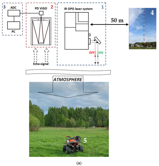
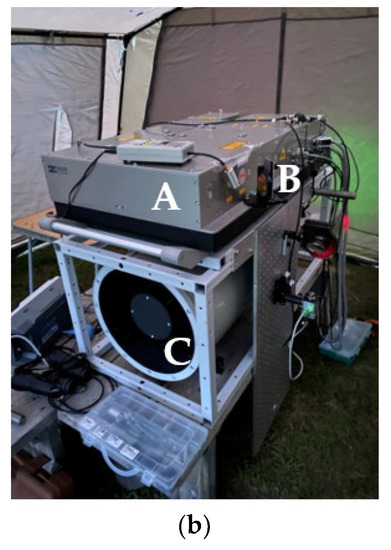
Figure 3.
(a) Scheme of in situ measurements of horizontally configured lidar with an output mirror: transmitter (1), receiver (2), and control and data acquisition and processing system (3), stationary post for measuring various meteorological parameters of the atmosphere, including the Picarro gas analyzer Picarro (4), and quad bike or all-terrain vehicle (AVT) with mirror reflector (5); (b) mobile IR lidar: laser with optical parametric oscillators (OPO) (A), output mirror (B), and receiving aperture of the telescope (C).
The reflector on the ATV was only used to check/adjust the alignment of the IR laser beam with the red alignment laser. With the use of a reflected red laser from a specular reflector, additional adjustment was carried out in the receiving part of the lidar; in particular, if necessary, the position of the sensitive area of the photodetector was adjusted along the red beam. Additionally, by using a red laser beam, it is possible to navigate on the direction of propagation of the laser radiation.
Following this, the ATV was removed from the route of the experiment; due to the output mirror, IR radiation was sent into the atmosphere, and on receiving the backscattered signal, it was still possible to adjust the position of the sensitive area of the photodetector in the receiving part using the amplitude of the echo signal on the oscilloscope. In order not to burn the sensitive photodiode in the receiving part or get rid of the lidar signal saturation mode, a set of light filters was used to reduce the energy of the output laser radiation.
2.4. Mobile Airborne Lidar System
2.4.1. Lidar Design
The modernized lidar for methane monitoring is a laser complex operating based on the lidar absorption and scattering method. The laser generates pulsed radiation with a pulse energy of up to 4.5 mJ at two wavelengths informative for the gas analysis. A laser beam is reflected from the first of flat mirrors and propagates through a set of color glasses (e.g., neutral density filters), which attenuates the output signal. Then, the laser beam is reflected from the second of the flat mirrors and propagates through the plane-parallel plate. A part of the beam energy is reflected towards the plane-convex lens, which focuses the radiation on the photosensitive area of the energy meter. The third of the flat mirrors guides the laser beam to the off-axis mirror collimator, after which the laser beam enters the atmosphere.
Part of the laser radiation is scattered while propagating through the atmosphere toward the Cassegrain telescope. The radiation collected by the telescope is guided by a flat mirror to the narrowband filter and then is recorded by the photodetector. The ratio of lidar signals recorded by the photodetector is used for retrieval of the atmospheric concentrations of the gas under study.
The lidar model and its components are shown in Figure 4, Figure 5 and Figure 6. Physical parameters of the lidar: sizes 1727.3 × 640 × 1184 mm, weight 150 kg.
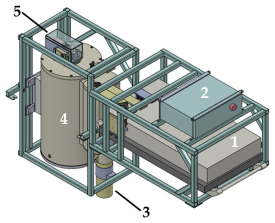
Figure 4.
Model of the modernized airborne lidar for atmospheric methane monitoring: laser (1); laser power unit (2); off-axis mirror collimator (3); Cassegrain telescope (4); photodetector unit (5).
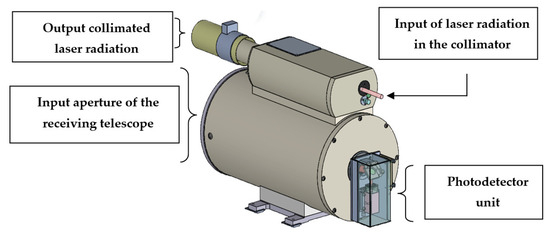
Figure 5.
Modernized transceiver of the mobile airborne lidar (collimator and receiving unit).
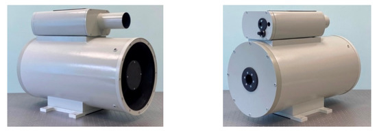
Figure 6.
Split system (collimator–receiving telescope) of the mobile airborne lidar.
While designing the airborne lidar, we used components which have shown their efficiency in previously created IR lidar systems [27,28,29]: flat mirrors, color glasses, energy meter, Cassegrain telescope, narrowband filter and photodetector. Parameters of the modernized lidar are given in Table 1.

Table 1.
Main parameters of the modernized airborne lidar.
2.4.2. Installation of a Lidar on Board an Aircraft
The modernized lidar was mounted onboard the TU-134 Optik aircraft laboratory of IAO SB RAS (Figure 7) [43].
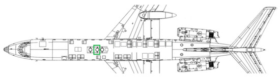
Figure 7.
Place of the mobile lidar (green rectangle) onboard the TU-134 “Optik” aircraft laboratory.
The lidar worked from an AC line (220 V, (50 ± 1) Hz) and was connected to a DC line (24 V) through a voltage converter. Before the use of the lidar, it was necessary to switch on the electronic components of the system. Then, it was necessary to start the lidar signal recording software and select a priori specifying system parameters (sensing wavelength, gas). After starting, the lidar operated in the autonomous mode.
The gas concentrations were retrieved by Equations (1) and (3). Data were saved on a memory card or HD of a PC during the lidar operation. The system operation was suspended via the software.
Thus, the mobile airborne lidar designed provides retrieval of spatially resolved vertical profiles of the methane content in the atmosphere and its integral values over vertical paths by the differential absorption method.
On 6 September 2022, the installation of the lidar on board the Tu-134 “Optik” aircraft laboratory of IAO SB RAS was carried out. Figure 8 shows the appearance of the onboard lidar. The lidar was equipped with two rechargeable batteries (capacity of 65 A/h each, total weight 45 kg) because it was necessary to maintain the thermal stabilization of the crystals in the OPO laser with the onboard power turned off when the aircraft was parked at night at the airport. Recharging the batteries was carried out by a special charger when the on-board power supply of the aircraft was running. Additionally, an additional tube was located at the output of the collimator to avoid illumination of the receiving part of the lidar and failure of the photodetector unit. This tube blocks diffused and high-intensity reflected radiation reflected from the glass of the aircraft hatch.
Figure 8.
(a) Photo of an airborne lidar; (b) transmitting aperture and additional tube (1) and receiving aperture (2) and aircraft hatch (3).
3. Results and Discussion
3.1. Simulation of the Lidar Overlap Function for Biaxial Scheme
The lidar overlap function was calculated with the aim of determining requirements for parameters of the receiving part of the mobile airborne system designed.
One of the important parameters of lidar systems is the overlap function (geometrical factor) of the lidar. The overlap function ξ(R) between the receiver field-of-view and a laser beam of a lidar system quantifies the range of the resolved number of photons reaching the detector normalized to the number of backscattered photons arriving on the telescope aperture. It mainly depends on the laser beam diameter, shape, and divergence, on the receiver parameters (telescope diameter, effective focal length, diameter of the field diaphragm, photodetector diameter), and on the relative position of the optical axes of the emitter and receiver [39,44,45,46,47].
When simulating the geometrical function of the biaxial scheme, parameters of the components of the optical scheme of transceiver (Table 2) were used. The photodetector radii were taken as equal to 0.1, 0.3, 0.5, 0.8 and 1 mm.
Table 2.
Input data for simulation of the geometrical function of the lidar.
It should be noted that in the case of using the classical scheme of the receiving lidar unit (consisting of a telescope, field diaphragm, collimating lens, band pass filter, interference (narrow band) filter, focusing lens, and photodetector), the field of view of the telescope is determined by the diameter of the field diaphragm [46]. In our particular (nontrivial) case, the receiving unit consisted of a telescope, a bandpass filter, an interference filter, and a photodetector. In this case, the field of view of the telescope was determined precisely by the diameter of the photodetector and there was no need to use a field diaphragm. The diameter of the photodetector area acted as the diaphragm aperture.
Based on the telescope parameters in Table 1 (diameter of primary mirror, effective focal length) for photodetectors of various sizes (0.1, 0.3, 0.5, 0.8 and 1 mm), the overlap function was calculated (Figure 9).
Figure 9.
Geometrical function (E) of the lidar accounting for the input parameters from Table 2 for a photodetector with the photosensitive area (a) 0.1, (b) 0.3, (c) 0.5, (d) 1 and (e) 0.8 mm radius (1—the calculation was carried out according to the formulas from [47], 2—the calculation was carried out according to the formulas from [39]).
Figure 9 shows the geometrical function (E) simulated with a maximum range (R) of 1000 m and input parameters of the lidar system transceiver from Table 2.
A software module in Python [48] was used for the calculation of the overlap function.
According to Figure 9, only partial overlap occurred along paths up to 1 km long for the photosensitive area radius 0.1, 0.3, and 0.5 mm.
The analysis of the simulation results (Figure 9d) shows that the linear recording zone started from a distance of 265 m when using photodiodes with a receiving zone diameter of 1 mm.
For the photodetector used in the developed lidar, the calculation of the overlap function was carried out using formulas from [47] and [39]. In the case of using a photodetector used in the developed lidar with a photosensitive zone radius of 0.8 mm (Figure 9d), the linear detection zone started from a distance of 390 m (calculation according to [39]), 400 m (calculation according to [47]). It is important to note that the geometrical function was equal to zero at a distance of 150 m for a biaxial lidar with the parameters specified and a laser beam propagating parallel to the telescope optical axis.
However, the numerical simulation results show a photodetector with a sensitive area of 1 mm diameter to be optimal for the receiving unit of a mobile lidar. This fact will be taken into account when improving the receiving part of the lidar system in future studies.
3.2. Simulation of Remote Sensing of Atmospheric Methane with a Mobile Onboard Lidar
To design a vertical version of the aircraft lidar and confirm its efficiency, we numerically simulated the remote gas analysis of the atmosphere under conditions of midlatitude and Arctic summer (corresponding to the aircraft expeditions scheduled for summer 2022–2023), with allowance for the parameters of key system components (laser, collimator, telescope, and photodetector) using the LIDA software [49].
The atmospheric gas concentration N(R) was retrieved by Equations (1) and (4). When retrieving the methane concentration by Equation (4), the albedo of the reflecting surface was assumed to be equal to 0.5.
The differential absorption cross-section was calculated with the use of the HITRAN database [35].
The main input parameters for the numerical simulation of the operation of the airborne lidar were: laser wavelengths (on- and off-line), laser pulse energy, pulse duration, pulse repetition rate, diameter of the primary mirror of the telescope, and parameters of the photodetector components (Table 3). Input value of the methane concentration to the simulation was 2.00–2.15 ppm. Sensing path was vertical downward.
Table 3.
Input data for simulation of airborne lidar operation.
To confirm the correct operation of the lidar under various environmental conditions, lidar signals were numerically simulated, and the spatial distribution and the integral methane content were then retrieved with the use of statistical models of temperature and atmospheric gases [50] and Equations (1) and (3).
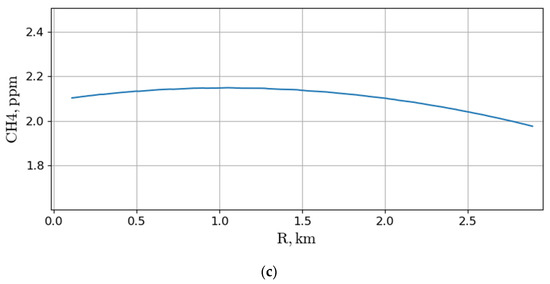
Figure 10.
(a) Atmospheric optical depth (OD) in the methane sounding informative range; (b) lidar signals (P, W); (c) spatial distribution of methane content retrieved from the numerical experiment with the atmospheric model of midlatitude summer.
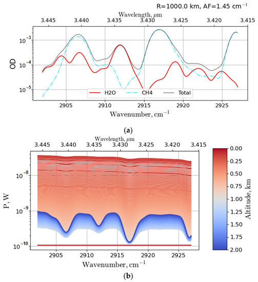
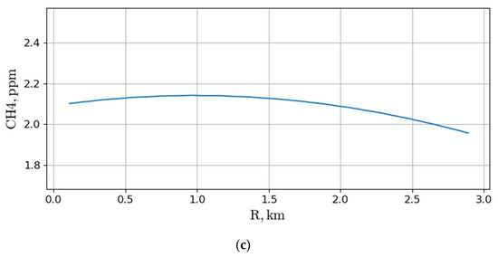
Figure 11.
(a) Atmospheric optical depth (OD) in the methane sounding informative range; (b) lidar signals (P, W); (c) spatial distribution of methane content retrieved from the numerical experiment with the atmospheric model of Arctic summer.
The numerical simulation confirmed the functionality of the modified airborne lidar under the meteorological conditions of midlatitude and Arctic summer.
Based on the optical depth simulation results (Figure 10a and Figure 11a), we selected emission (absorption) on- and off-line wavelengths from the methane sounding informative range, which are the most suitable for sounding under the conditions of midlatitude summer (2916.55 cm−1 on-line and 2915.00 cm−1 off-line) and polar (2917.00 cm−1 on-line and 2915.00 cm−1 off-line). The lidar signals (Figure 10b and Figure 11b) received in the methane sounding informative range did not exceed the photodetector NEP values (~10−10 W) and were sufficient to retrieve the gas concentration. The spatially distributed methane content retrieved varied in the 1.975–2.150 ppm range along a vertical path 3 km long under meteorological conditions of midlatitude summer (Figure 10c) (the retrieval error was 0.175 ppm); the integral methane content retrieved was 2.14 ppm. Under the meteorological conditions of Arctic summer (Figure 11c), the value varied in the 1.95–2.14 ppm range (the retrieval error was 0.19 ppm); the integral methane content retrieved was 2.12–2.13 ppm. The methane content values retrieved from the numerical experiment did not contradict the methane trend in 2022 [51].
3.3. Experimental Results Using Ground-Based Mobile Lidar System
During the experiments, we used a horizontal lidar configuration with an output mirror (see Figure 3b), which made it possible to specify the laser radiation direction.
Laser radiation at informative wavelengths of methane monitoring was directed to the output mirror and redirected into the atmosphere, as shown in Figure 3a. To ensure complete coverage of the laser beam and the field of view of the telescope in the near field, the beams were deflected from the optical axis of the telescope. The backscattered signals were collected by a receiving telescope. The photodetector in the receiving part of the lidar recorded backscattered signals at on- and off-line wavelengths of methane sounding. From the ratio of lidar signals, the concentration on the studied sounding path was restored.
Figure 12 shows the results of in situ tests of the ground-based lidar. The lidar signals received (Figure 12a,b) confirm the correct automated operation of the receiving part of the system and the differential absorption sufficient for retrieving the methane content. During the test tests, the limitation of the sounding path and a sharp decrease in the signal were due to the loss of the laser beam from the field of view of the telescope at a distance of more than 500 m. Background values of the methane content retrieved from the experiment along a 500 m horizontal path are shown in Figure 12c.
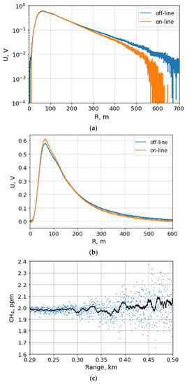
Figure 12.
Lidar signals (U, V) at methane sounding informative wavelengths in (a) logarithmic form, (b) linear form; (c) average methane content retrieved from lidar signals.
The methane content values at the experimental site varied within a background value of 1.95–2.10 ppm. The results of lidar measurements were compared with the measurements of the Picarro gas analyzer. For a quantitative comparison of the results of lidar measurements with the data of the Picarro gas analyzer, the experimental values of the CH4 content in the atmosphere obtained by two methods (lidar, in situ) are given in Table 4.
Table 4.
Results of lidar measurements at Tomsk region and comparison with the results of in situ measurements of Picarro gas analyzer.
Thus, as the measurement results show in Figure 12c and in Table 4, the data obtained by the lidar method are in satisfactory agreement (for part of the sounding path 200–400 m) with the data of the Picarro gas analyzer, which was equipped with a stationary station for measuring meteorological parameters of the atmosphere. However, for more accurate verification of lidar measurements of methane concentration, it is necessary to place the Picarro mobile gas analyzer at fixed points along the path of propagation of laser radiation. Placing a Picarro mobile gas analyzer on the sounding path would give a more accurate picture, especially for ranges >400 m. This fact will be taken into account by the authors of the work when conducting future studies on a horizontal (inclined) sounding path.
The test results allowed us to develop requirements for further upgrades of the mobile lidar in order to expand the measurement range, improve the stability of the output parameters of the lidar radiation source, increase the sensitivity of the detectors in the receiving part of the lidar, create a vertical configuration for sounding from an aircraft, and use it in Arctic summer latitudes.
3.4. Collimated Laser Beam and Stability of the Laser Radiation Pulse Output Energy of the Mobile Airborne Lidar System
The results of the numerical simulation of remote vertical methane monitoring and in situ experiments on the study of atmospheric methane along surface paths with the mobile lidar system were used to upgrade the system for aircraft sounding conditions.
Figure 13 shows the beam shape of the alignment laser (630 nm) at the entrance of and exit from the off-axis collimator. The collimator ensured a four-fold decrease in the laser radiation divergence (methane sounding informative on- and off-lines).
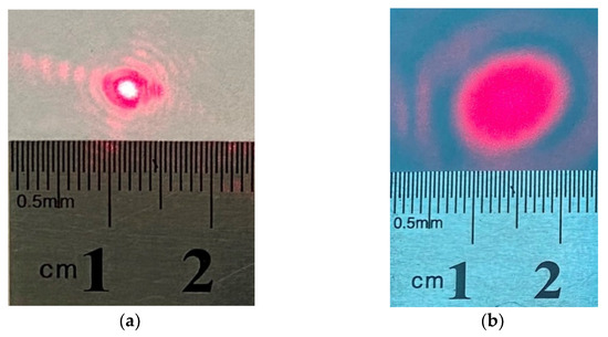
Figure 13.
Alignment laser beam at the (a) entrance of and (b) exit from the collimator.
The stability of output pulse energy was estimated during the alignment/tuning of the lidar laser in the methane sounding informative range (2916.55–2917 cm−1 on-line and 2915.00 cm−1 off-line). The measurements were carried out in the test mode of the operation of the lidar radiation source in turn on each of the informative probing lines at a pulse repetition rate of 10 Hz. The accumulation time of ~6000 pulses was 10 min. The measurement results are shown in Figure 14.
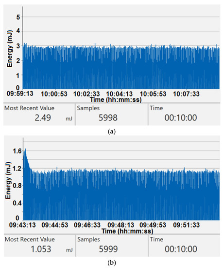
Figure 14.
Stability of the laser radiation pulse output energy of the airborne lidar in the methane sounding informative wavelength range: (a) 2916.55–2917 cm−1 on-line; (b) 2915.00 cm−1 off-line.
The results confirm the stable operation of the laser source at wavelengths required for in situ lidar measurements when calibration equipment is absent. The energy burst in Figure 14b corresponds to the ramp-up time of the laser.
3.5. First Test Flights and Measurement Results
On 6–11 September 2022, the planned flight expedition of the IAO SB RAS took place on the Tu-134 “Optik” aircraft laboratory along the route Novosibirsk–Salekhard–Kara Sea–Salekhard–Tomsk. For the first time, a lidar was installed on board an aircraft laboratory to measure methane. The lidar monitoring scheme from the aircraft laboratory is shown in Figure 15.
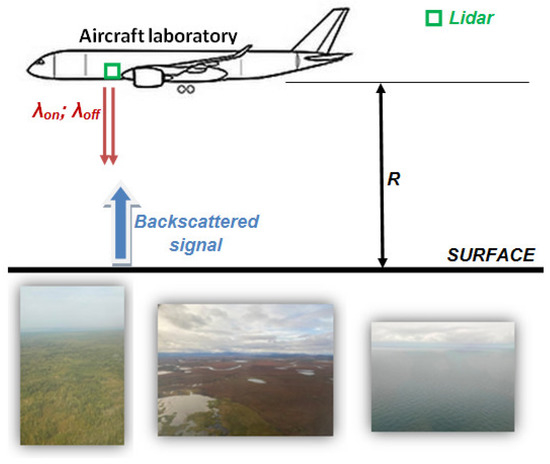
Figure 15.
The lidar monitoring scheme from the aircraft laboratory (λon; λoff—informative wavelengths of methane monitoring; R—monitoring path (range)).
Experimental measurements were carried out (probing path vertically down through the aircraft hatch) and a large amount of experimental data of methane lidar sounding at different aircraft flight altitudes (0.2–11 km) was accumulated. In this paper, we restricted ourselves to the altitude interval of an aircraft flight of 0.265–3 km, for which the numerical simulation presented in Section 3.2 was carried out. The main points of the aircraft flight route and home airports are shown in Figure 16 [52]. Figure 16 also shows photographs from the measurement site. Three local points were selected (in Figure 16—orange triangles) for measurements near the Novosibirsk airport (the point of measurements corresponds to the conditions of midlatitude summer), the coastal part and the water area of the Kara Sea (the point of measurements corresponds to the conditions of the Arctic summer).
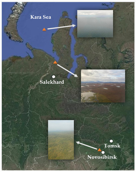
Figure 16.
A map of methane measurements using an onboard lidar during a flight expedition (three points (orange triangles) were selectively taken from the array of experimental data obtained: Novosibirsk—midlatitude summer, Salekhard, in particular, locations of the coastal part and water area of the Kara Sea—Arctic summer).
Figure 17 shows the average CH4 concentrations recovered from lidar signals over a 100 s aircraft flight at an altitude of 2000–3000 m near Novosibirsk airport (a); at an altitude of 380 m above the coastal part near the Kara Sea (b); at an altitude of 270 m above the water part of the Kara Sea (c).
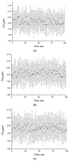
Figure 17.
Average CH4 concentration (black dots) reconstructed from lidar signals at informative wavelengths (a) under midlatitude summer conditions during an aircraft flight at an altitude of 2000–3000 m near Novosibirsk; (b) in Arctic summer conditions when the aircraft was flying at an altitude of 380 m above the coastal part near the Kara Sea; (c) conditions of the Arctic summer during the aircraft flight at an altitude of 270 m above the water area of the Kara Sea.
The flight at different aircraft altitudes was carried out for different amounts of time; in some cases there was a climb, and in some cases the aircraft flew at the same altitude for up to 7 min. The time period of 100 s was taken for convenience and uniformity of displaying in Figure 17 the obtained values of experimental studies; that is, so that the X-axis has the same measurement range in time.
The aircraft was also equipped with a Picarro gas analyzer, which made it possible to compare the data of lidar measurements of the methane concentration presented in Figure 17a–c with local measurements of the methane concentration, which for the case of an aircraft flying at an altitude of 2000–3000 m near Novosibirsk varied within values of 2.01–2.02 ppm; for the case of an aircraft flying at an altitude of 380 m above the coastal part near the Kara Sea, it varied within the range of 2.00–2.01 ppm; and for the case of an aircraft flying at an altitude of 270 m above the water area of the Kara Sea, it was 1.98 ppm. An analysis of the data from the lidar and local measurements of methane showed that the RMS error in reconstructing the average methane concentration in all three cases of lidar measurements was less than 7% (bias was 11–14.1%). For a quantitative comparison of the results of lidar measurements with the data of the Picarro gas analyzer, obtained by two methods (lidar—average values of the CH4 concentration, in situ—local values of the CH4 concentration), the experimental values of CH4 content in the atmosphere are given in Table 5.
Table 5.
Results of lidar measurements at selected locations and comparison with the results of in situ measurements of the Picarro gas analyzer.
4. Conclusions
A mobile lidar has been modernized for the tasks of airborne monitoring of methane content in the atmosphere. The lidar is retrofitted with an off-axis mirror collimator, which makes it possible to reduce the divergence of the output laser radiation by a factor of 4. The results of the simulation of the lidar overlap function are presented. Based on the simulation results, additional requirements were determined for the parameters of the lidar designed for atmospheric research and methane monitoring. It is shown that when using photodetectors with a sensitive area radius of 0.8 mm, the lidar signals can be recorded beginning from a distance of 390 m. The results of simulation of methane sounding for the conditions of midlatitude and Arctic summer, which correspond to the conditions of the flight expeditions scheduled for 2022–2023, were analyzed. They confirm a possibility of retrieving the methane content close to the background value (~2 ppm). The lidar design for methane monitoring in the troposphere is described. A lidar for methane monitoring was installed on board the Tu-134 “Optik” aircraft laboratory. The experimental results obtained during the testing of the onboard lidar show the possibility of recovering the averaged methane concentration from the lidar signals backscattered at informative sounding wavelengths under mid-latitude and Arctic summer conditions.
Author Contributions
Conceptualization, methodology, formal analysis, writing—original draft preparation, writing—review and editing, S.V.Y.; conceptualization, software, visualization, validation S.A.S.; resources, project administration, funding acquisition, O.A.R. All authors have read and agreed to the published version of the manuscript.
Funding
The work was supported by the Ministry of Science and Higher Education of the Russian Federation (project “Study of anthropogenic and natural factors changes in the composition of air and environmental objects in Siberia and Russian sector of the Arctic in the face of rapid climate change with using the unique scientific installation Tu-134 “Optik” aircraft laboratory” agreement no. 075-15-2021-934).
Data Availability Statement
Not applicable.
Acknowledgments
The authors are grateful to B.D. Belan, the head of the Atmosphere Composition Climatology of IAO SB RAS.
Conflicts of Interest
The authors declare no conflict of interest.
References
- WMO. Greenhouse Gas Bulletin, 15. Available online: https://public.wmo.int/en/resources/library/wmo-greenhouse-gas-bulletin-no-15 (accessed on 12 February 2022).
- Yerasi, A.; Tandy, W.D.; Emery, W.J.; Barton-Grimley, R.A. Comparing the theoretical performances of 1.65- and 3.3-μm differential absorption lidar systems used for airborne remote sensing of natural gas leaks. J. Appl. Remote Sens. 2018, 12, 026030. [Google Scholar] [CrossRef]
- Bartholomew, J.; Lyman, P.; Weimer, C.; Tandy, W. Wide area methane emissions mapping with airborne IPDA lidar. Proc. SPIE 2017, 10406, 1040607. [Google Scholar] [CrossRef]
- Michael, F.B.; Richard, W.T.; Matthew, L.C.; Mark, A.G.; James, R.; Paul, W.; Sean, D.; John, G.; Ron, C.; Daniele, P.; et al. Low-cost lightweight airborne laser-based sensors for pipeline leak detection and reporting. Proc. SPIE 2013, 8726, 87260C. [Google Scholar] [CrossRef]
- Horn, B. ALMA provides smarter gas pipeline aerial survey. Pipeline Gas J. 2014, 241, 96. [Google Scholar]
- Amediek, A.; Ehret, G.; Fix, A.; Wirth, M.; Budenbender, C.; Quatrevalet, M.; Kiemle, C.; Gerbig, C. CHARM-F—A new airborne integrated-path differential-absorption lidar for carbon dioxide and methane observations: Measurement performance and quantification of strong point source emissions. Appl. Opt. 2017, 56, 5182–5197. [Google Scholar] [CrossRef]
- Degtiarev, E.V.; Geiger, A.R.; Richmond, R.D. Compact mid-infrared DIAL lidar for ground-based and airborne pipeline monitoring. Proc. SPIE 2003, 4882, 432–442. [Google Scholar] [CrossRef]
- Murdock, D.G.; Stearns, S.V.; Lines, R.; Lenz, D.; Brown, D.M.; Philbrick, C.R. Applications of real-world gas detection: Airborne Natural Gas Emission Lidar (ANGEL) system. J. Appl. Remote Sens. 2008, 2, 023518. [Google Scholar]
- Fix, A.; Ehret, G.; Hoffstädt, A.; Klingenberg, H.; Lemmerz, C.; Mahnke, P.; Ulbricht, M.; Wittig, R.; Zirnig, W. CHARM—A helicopter-borne lidar system for pipeline monitoring. In Proceedings of the 22nd International Laser Radar Conference (ILRC 2004), Matera, Italy, 12–16 July 2004; pp. 45–48. [Google Scholar]
- Meng, L.; Fix, A.; Wirth, M.; Høgstedt, L.; Tidemand-Lichtenberg, P.; Pedersen, C.; Rodrigo, P.J. Upconversion detector for range-resolved DIAL measurement of atmospheric CH4. Opt. Express 2018, 26, 3850–3860. [Google Scholar] [CrossRef]
- Wagner, G.A.; Plusquellic, D.F. Ground-based, integrated path differential absorption LIDAR measurement of CO2, CH4, and H2O near 1.6 mum. Appl. Opt. 2016, 55, 6292–6310. [Google Scholar] [CrossRef]
- Kara, O.; Sweeney, F.; Rutkauskas, M.; Farrell, C.; Leburn, C.G.; Reid, D.T. Open-path multi-species remote sensing with a broadband optical parametric oscillator. Opt. Express 2019, 27, 21358–21366. [Google Scholar] [CrossRef]
- Innocenti, F.; Robinson, R.; Gardiner, T.; Finlayson, A.; Connor, A.J.R.S. Differential absorption lidar (DIAL) measurements of landfill methane emissions. Remote Sens. 2017, 9, 953. [Google Scholar] [CrossRef]
- Emission Monitoring Using Differential Absorption Lidar (DIAL). Available online: https://www.npl.co.uk/products-services/environmental (accessed on 10 May 2022).
- Riris, H.; Numata, K.; Li, S.; Wu, S.; Ramanathan, A.; Dawsey, M.; Mao, J.; Kawa, R.; Abshire, J.B. Airborne measurements of atmospheric methane column abundance using a pulsed integrated-path differential absorption lidar. Appl. Opt. 2012, 51, 8296–8305. [Google Scholar] [CrossRef]
- Riris, H.; Numata, K.; Wu, S.; Gonzalez, B.; Rodriguez, M.; Scott, S.; Kawa, S.; Mao, J. Methane optical density measurements with an integrated path differential absorption lidar from an airborne platform. J. Appl. Remote Sens. 2017, 11, 034001. [Google Scholar] [CrossRef]
- Fix, A.; Amediek, A.; Büdenbender, C.; Ehret, G.; Quatrevalet, M.; Wirth, M.; Löhring, J.; Kasemann Klein, R.J.; Hoffmann, H.-D.; Klein, V. Development and First Results of a new Near-IR Airborne Greenhouse Gas Lidar. In Proceedings of the Advanced Solid State Lasers Conference, OSA 2015, Berlin, Germany, 4–9 October 2015. [Google Scholar] [CrossRef]
- Fix, A.; Amediek, A.; Bovensmann, H.; Ehret, G.; Gerbig, C.; Gerilowski, K.; Pfeilsticker, K.; Roiger, A.; Zöger, M. CoMet: An airborne mission to simultaneously measure CO2 and CH4 using lidar, passive remote sensing, and in-situ techniques. In Proceedings of the 28th International Laser Radar Conference (ILRC 28), Bucharest, Romania, 25–30 June 2017; Volume 176, p. 02003. [Google Scholar] [CrossRef]
- Galkowski, M.; Jordan, A.; Rothe, M.; Marshall, J.; Koch, F.-T.; Chen, J.; Agusti-Panareda, A.; Fix, A.; Gerbig, C. In situ observations of greenhouse gases over Europe during the CoMet 1.0 campaign aboard the HALO aircraft. Atmos. Meas. Tech. 2021, 14, 1525–1544. [Google Scholar] [CrossRef]
- Fiehn, A.; Kostinek, J.; Eckl, M.; Klausner, T.; Galkowski, M.; Chen, J.; Gerbig, C.; Röckmann, T.; Maazallahi, H.; Schmidt, M.; et al. Estimating CH4, CO2 and CO emissions from coal mining and industrial activities in the Upper Silesian Coal Basin using an aircraft-based mass balance approach. Atmos. Chem. Phys. 2020, 20, 12675–12695. [Google Scholar] [CrossRef]
- Nickl, A.L.; Mertens, M.; Roiger, A.; Fix, A.; Amediek, A.; Fiehn, A.; Gerbig, C.; Galkowski, M.; Kerkweg, A.; Klausner, T.; et al. Hindcasting and forecasting of regional methane from coal mine emissions in the Upper Silesian Coal Basin using the online nested global regional chemistry-climate model MECO(n) (MESSy v2.53). Geosci. Model Dev. 2020, 13, 1925–1943. [Google Scholar] [CrossRef]
- Kostinek, J.; Roiger, A.; Eckl, M.; Fiehn, A.; Luther, A.; Wildmann, N.; Klausner, T.; Fix, A.; Knote, C.; Stohl, A.; et al. Estimating Upper Silesian coal mine methane emissions from airborne in situ observations and dispersion modeling. Atmos. Chem. Phys. 2021, 21, 8791–8807. [Google Scholar] [CrossRef]
- Pierangelo, C.; Millet, B.; Esteve, F.; Alpers, M.; Ehret, G.; Flamant, P.; Berthier, S.; Gibert, F.; Chomette, O.; Edouart, D.; et al. 2015: MERLIN (Methane Remote Sensing Lidar Mission): An Overview. In Proceedings of the 27th International Laser Radar Conference ILRC, New York, NY, USA, 5–10 July 2015. [Google Scholar]
- Nikolov, S.; Wührer, C.; Kühl, C.; Bode, M.; Hupfer, W.; Lucarelli, S. MERLIN: Design of an IPDA LIDAR instrument. CEAS Space J. 2019, 11, 437–457. [Google Scholar] [CrossRef]
- Philipp, M.; Dietz, A.; Buchelt, S.; Kuenzer, C. Trends in satellite earth observation for permafrost related analyses-a review. Remote Sens. 2021, 13, 1217. [Google Scholar] [CrossRef]
- Barton-Grimley, R.A.; Nehrir, A.R.; Kooi, S.A.; Collins, J.E.; Harper, D.B.; Notari, A.; Lee, J.; DiGangi, J.P.; Choi, Y.; Davis, K.J. Evaluation of the High Altitude Lidar Observatory (HALO) methane retrievals during the summer 2019 ACT-America campaign. Atmos. Meas. Tech. 2022, 15, 4623–4650. [Google Scholar] [CrossRef]
- Yakovlev, S.; Sadovnikov, S.; Kharchenko, O.; Kravtsova, N. Remote Sensing of Atmospheric Methane with IR OPO Lidar System. Atmosphere 2020, 11, 70. [Google Scholar] [CrossRef]
- Romanovskii, O.A.; Sadovnikov, S.A.; Kharchenko, O.V.; Yakovlev, S.V. Remote Analysis of Methane Concentration in the Atmosphere with an IR Lidar System in the 3300–3430 nm Spectral Range. Atmos. Ocean. Opt. 2020, 33, 188–194. [Google Scholar] [CrossRef]
- Romanovskii, O.A.; Sadovnikov, S.A.; Yakovlev, S.V.; Tuzhilkin, D.A.; Kharchenko, O.V.; Kravtsova, N.S. Mobile 3.4–µm differential absorption lidar system for remote sensing of the atmospheric methane. Proc. SPIE 2021, 11916, 119161T. [Google Scholar] [CrossRef]
- Collis, R.T.H.; Russell, P.B. Lidar Measurement of Particles and Gases by Elastic Backscattering and Differential Absorption; Springer: New York, NY, USA, 1976; pp. 91–180. [Google Scholar] [CrossRef]
- Ismail, S.; Browell, E.V. LIDAR Differential Absorption Lidar. In Encyclopedia of Atmospheric Sciences, 2nd ed.; Elsevier: Amsterdam, The Netherlands, 2015; pp. 277–288. [Google Scholar] [CrossRef]
- Vasil’ev, B.I.; Mannoun, U.M. IR differential-absorption lidars for ecological monitoring of the environment. Quantum Electron. 2006, 36, 801–820. [Google Scholar] [CrossRef]
- Weitkamp, C. Lidar: Range-Resolved Optical Remote Sensing of the Atmosphere; Springer Science & Business: Berlin/Heidelberg, Germany, 2006; Volume 102. [Google Scholar] [CrossRef]
- Li, J.; Yu, Z.; Du, Z.; Ji, Y.; Liu, C. Standoff chemical detection using laser absorption spectroscopy. Remote Sens. 2020, 12, 2771. [Google Scholar] [CrossRef]
- Gordon, I.E.; Rothman, L.S.; Hargreaves, R.J.; Hashemia, R.; Karlovetsa, E.V.; Skinnera, F.M.; Conwaya, E.K.; Hillb, C.; Kochanovacd, R.V.; Tan, Y.; et al. The HITRAN2020 molecular spectroscopic database. J. Quant. Spectr. Radiat. Transfer. 2022, 277, 107949. [Google Scholar] [CrossRef]
- Babchenko, S.V.; Matvienko, G.G.; Sukhanov, A.Y. Assessing the possibilities of sensing CH4 and CO2 greenhouse gases above the underlying surface with satellite-based IPDA lidar. Atmos. Ocean. Opt. 2015, 28, 245–253. [Google Scholar] [CrossRef]
- Matvienko, G.G.; Sukhanov, A.Y. Application of Neural Networks for Retrieval of the CO2 Concentration at Aerospace Sensing by IPDA-DIAL lidar. Remote Sens. 2019, 11, 659. [Google Scholar] [CrossRef]
- Halldórsson, T.; Langerholc, J. Geometrical form factors for the lidar function. Appl. Opt. 1978, 17, 240–244. [Google Scholar] [CrossRef]
- Measures, R.M. Laser Remote Sensing Fundamentals and Applications; John Wiley & Sons, Inc.: Hoboken, NJ, USA, 1984. [Google Scholar]
- Refaat, T. Advanced Atmospheric Water Vapor Dial Detection System. Ph.D. Thesis, Electrical & Computer Engineering, Old Dominion University, Norfolk, VA, USA, 2000. [Google Scholar] [CrossRef]
- Yakovlev, S.V.; Romanovskii, O.A.; Sadovnikov, S.A.; Tuzhilkin, D.A.; Nevzorov, A.A.; Kharchenko, O.V.; Kravtsova, N.S. Mobile mid-infrared differential absorption lidar for methane monitoring in the atmosphere: Calibration and first in situ tests. Results Opt. 2022, 8, 100233. [Google Scholar] [CrossRef]
- Available online: https://lop.iao.ru/EN/ (accessed on 5 June 2021).
- Anokhin, G.G.; Antokhin, P.N.; Arshinov, M.Y.; Barsuk, V.E.; Belan, B.D.; Belan, S.B.; Davydov, D.K.; Ivlev, G.A.; Inoue, G.; Kozlov, A.V.; et al. Aircraft laboratory Tu-134 “Optic”. Atmos. Ocean. Opt. 2011, 24, 805–816. (In Russian) [Google Scholar]
- Sicard, M.; Rodriguez-Gomez, A.; Comeron, A.; Munoz-Porcar, C. Calculation of the Overlap Function and Associated Error of an Elastic Lidar or a Ceilometer: Cross-Comparison with a Cooperative Overlap-Corrected System. Sensors 2020, 20, 6312. [Google Scholar] [CrossRef]
- Bobrovnikov, S.M.; Gorlov, E.V.; Zharkov, V.I. A Multi-Aperture Transceiver System of a Lidar with Narrow Field of View and Minimal Dead Zone. Atmos. Ocean. Opt. 2018, 31, 690–697. [Google Scholar] [CrossRef]
- Stelmaszczyk, K.; Dell’Aglio, M.; Chudzyński, S.; Stacewicz, T.; Wöste, L. Analytical function for lidar geometrical compression form-factor calculations. Appl. Opt. 2005, 44, 1323–1331. [Google Scholar] [CrossRef]
- Kuze, H.; Kinjo, H.; Sakurada, Y.; Takeuchi, N. Field-ofview dependence of lidar signals by use of Newtonian and Cassegrainian telescopes. Appl. Opt. 1998, 37, 3128–3132. [Google Scholar] [CrossRef]
- Available online: https://www.python.org (accessed on 20 April 2022).
- Sadovnikov, S.A. Software system for numerical simulation of broadband laser gas analysis of the atmosphere. Inf. Control Syst. 2018, 97, 66–73. [Google Scholar] [CrossRef]
- Zuev, V.E.; Komarov, V.S. Statistical Models of the Temperature and Gaseous Components of the Atmosphere; Gidrometeoizdat: Leningrad, Russia, 1986. [Google Scholar]
- Available online: https://gml.noaa.gov/ccgg/trends_ch4/ (accessed on 30 May 2022).
- Available online: https://www.google.ru/maps/ (accessed on 10 October 2022).


Publisher’s Note: MDPI stays neutral with regard to jurisdictional claims in published maps and institutional affiliations. |
© 2022 by the authors. Licensee MDPI, Basel, Switzerland. This article is an open access article distributed under the terms and conditions of the Creative Commons Attribution (CC BY) license (https://creativecommons.org/licenses/by/4.0/).