Abstract
Thermal mapping of surface waters and the land surface via UAVs offers exciting opportunities in many scientific disciplines; however, unresolved issues persist related to accuracy and drift of uncooled microbolometric thermal infrared (TIR) sensors. Curiously, most commercially available UAV-based TIR sensors are black, which will theoretically facilitate heating of the uncooled TIR sensor via absorbed solar radiation. Accordingly, we tested the hypothesis that modifying the surface absorptivity of uncooled TIR sensors can reduce thermal drift by limiting absorptance and associated microbolometer heating. We used two identical uncooled TIR sensors (DJI Zenmuse XT2) but retrofitted one with polished aluminum foil to alter the surface absorptivity and compared the temperature measurements from each sensor to the accurate measurements from instream temperature loggers. In addition, because TIR sensors are passive and measure longwave infrared radiation emitted from the environment, we tested the hypotheses that overcast conditions would reduce solar irradiance, and therefore induce thermal drift, and that increases in air temperature would induce thermal drift. The former is in contrast with the conceptual model of others who have proposed that flying in overcast conditions would increase sensor accuracy. We found the foil-shielded sensor yielded temperatures that were on average 2.2 °C more accurate than those of the matte black sensor (p < 0.0001). Further, we found positive correlations between light intensity (a proxy for incoming irradiance) and increased sensor accuracy for both sensors. Interestingly, light intensity explained 73% of the accuracy variability for the black sensor, but only 40% of the variability in accuracy deviations for the foil-shielded sensor. Unsurprisingly, an increase in air temperature led to a decrease in accuracy for both sensors, where air temperature explained 14% of the variability in accuracy for the black sensor and 31% of the accuracy variability for the foil-shielded sensor. We propose that the discrepancy between the amount of variability explained by light intensity and air temperature is due to changes in the heat energy budget arising from changes in the surface absorptivity. Additionally, we suggest fine-scale changes in river-bed reflectance led to errors in UAV thermal measurements. We conclude with a suite of guidelines for increasing the accuracy of uncooled UAV-based thermal mapping.
1. Introduction
Thermal mapping of surface waters and the land surface via UAVs offers exciting opportunities in many disciplines including ecology, hydrology, hydrogeology, and oceanography [1,2,3]; however, there are unresolved issues related to accuracy and drift of uncooled thermal infrared (TIR) sensors. TIR imaging, or thermography, began in the mid-19th century with William Herschel’s finding that light radiates heat. In 1954 the first IR sensor was constructed, and in 1960 Texas Instruments built the first forward looking infrared system (FLIR) [4]. By 1995, uncooled microbolometers (a type of IR sensor) were developed. The development of TIR sensors of various sizes has facilitated their deployment on both spaceborne and airborne platforms (Figure 1a,b, respectively). Many satellite platforms, such as LandSat 8 and Sentinel 3, are equipped with IR sensors allowing accurate and repeated measurements of the temperature of Earth’s surface and large waterbodies [5,6,7], and facilitating global studies on temperature-induced forest and agricultural crop stresses. TIR sensors on aeroplanes and helicopters have detailed high spatial resolution riverine thermal heterogeneity at the riverscape scale [8,9], enabling researchers to develop new concepts to explain the spatial variability of river thermal regimes at the catchment-scale [10,11]. In the last decade, UAV-based TIR sensors have become increasingly common in river research and applications (Figure 1c,e) (e.g., [12,13,14]). The relatively recent development of UAV-based TIR sensing affords scientists, researchers and practitioners the potential to examine abiotic and biotic processes across fine to broad spatial scales, and the relatively low cost of UAV-based TIR sensors is providing new insights into ecosystem processes [15,16,17,18].
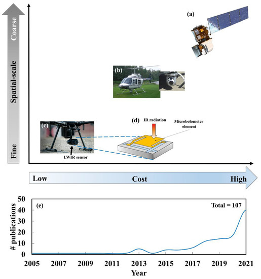
Figure 1.
A schematic detailing the thermal infrared (TIR) sensors that are used from coarse to fine spatial-scales and their correspondent costs ((a)satellite, (b) airborne, and (c) UAV-based). (d) A simple conceptual model of a microbolometer. The increase in number of publications with the keywords (UAV + TIR) from a SCOPUS database search is illustrated in (e).
Two seminal studies by [19,20] on mapping sub-metre resolution river thermal heterogeneity via airborne TIR underpinned a steady increase in the use of TIR in freshwater systems to investigate hydrology [10,21,22,23], hydrogeology [24,25], ecology [26,27,28,29,30], and ecohydraulics [15]. Whilst cooled TIR sensors, such as quantum well infrared photon detectors which are expensive and too large for typical UAV payloads, have proven to be highly accurate for mapping river temperatures, e.g., [10,20,21,31], findings on the accuracy of uncooled TIR sensors, such as those used for UAV TIR mapping campaigns, have been mixed. For instance, [9] used a helicopter-mounted uncooled TIR sensor to map river temperature in New Brunswick, Canada and reported excellent relationships between sensor-derived temperatures (termed radiant temperature, or TR) and river temperature (termed kinetic temperature, or TK). Similarly, [32] found strong agreement between uncooled TIR TR and TK. However, a recent study by [33] reported extensive thermal drift in TR measurements from a UAV-based uncooled TIR sensor in contrast to TK. This thermal drift has also been reported by others using different UAV-based microbolometric TIR sensors see [34,35,36,37].
All TIR sensors are passive, they measure the radiation emitted from an object. For environmental studies the long-wave infrared radiation (LWIR) region of the electromagnetic spectrum (8–15 µm) is most typically measured. Of the available IR sensor types, currently only microbolometers (i.e., resistors used as detectors in TIR sensors) meet the lightweight criterion for UAV operation. Furthermore, microbolometers are the most commonly available thermal imagers [38]. Microbolometers create TIR images via the bolometric effect, defined as a change in the electrical resistance of a material due to temperature increases caused by absorbed radiation (Figure 1d). As more incident LWIR energy is absorbed by the microbolometer element, the electrical resistance of the material increases [4,38]. Electrical resistance variability can be measured by passing a current through the instrument, and the resistance changes can be converted to temperature to develop a TIR image [39]. The temperature dependence of electrical resistance also underpins one of the main disadvantages of using uncooled microbolometers: variability in heat energy exchanges both internally, i.e., operational heat gains, and externally, i.e., solar irradiance and air temperature, can lead to thermal drift [39,40].
The number of studies employing UAV-based TIR sensors has risen rapidly over the last 5 years (Figure 1e). The use of these TIR sensors is aiding and augmenting our understanding of groundwater–surface water exchanges [25], the role of thermodynamics and hydraulics on fish habitat use [15], and the identification of thermal heterogeneity at the reach scale [41,42]. Nonetheless, [33] highlighted that whilst UAV-based uncooled TIR sensors can be used to identify discrete thermal heterogeneity, they can suffer from extensive thermal drift and therefore their capacity to accurately characterize thermal patterns is impinged. This presents a substantial pitfall when using uncooled UAV-based TIR sensors for applications that require accurate temperatures, such as hydrological studies where temperature is used as a tracer [12,24,25,43], or ecological studies examining the role of temperature on freshwater biota [30]. Calibration algorithms have been developed to address these limitations [35,44], but these calibration techniques do not address one of the primary drivers of thermal drift: microbolometer temperature. [33] proposed that UAV-based TIR thermal drift could be limited by conducting missions during overcast conditions. Here, we tested the hypothesis that modifying the surface absorptivity of uncooled TIR sensors can reduce thermal drift by limiting absorptance and thereby microbolometer heating. We used two identical uncooled TIR sensors but retrofitted one with polished aluminum foil to alter the absorptivity. We then compared TIR images from each sensor to accurate measurements from instream temperature loggers. In addition, since TIR sensors are passive, we hypothesized that overcast conditions would decrease the signal to noise ratio, as less LWIR would reach the sensor, and therefore, lead to greater thermal drift, in contrast with the conceptual model of others. Finally, we hypothesized that increases in air temperature would induce thermal drift—with the acknowledgement that low air temperatures can be associated with clear sky conditions. To test these hypotheses, we collected light intensity and air temperature data and conducted statistical analyses. Findings from this study are relevant to many scientific disciplines interested in the application of UAV-based uncooled TIR sensors to characterize and elucidate environmental thermal patterns.
2. Methods
2.1. Study Site
The study was conducted on the Nashwaak River in central New Brunswick, Canada (Figure 2a). The Nashwaak River drains ~1700 km2 and occupies two physiographic regions: the Miramichi Highlands and the Maritime Plains [45]. Historically the Nashwaak River was an excellent Atlantic salmon (Salmo salar) fishery; however, that population is now endangered. The study site is a 180 m river reach that is characterized by riffles and runs in the upstream and mid-stream sections and transitions into a pool in the downstream section (Figure 2b). The reach also includes discharge from Ryan Brook (Figure 2b). Ryan Brook drains an area with highly incised valleys underlain by shallow, hydraulically conductive clastic sedimentary bedrock [46], and similar to other areas in the region, the coupling of valley incision and shallow, hydraulically conductive bedrock leads to a dominance of diffusive groundwater discharge [11,24]. Importantly for this study, the confluence of the groundwater-dominant inflow of Ryan Brook with the warm Nashwaak River provides thermal heterogeneity to examine the accuracy of each sensor treatment across a range of temperatures.
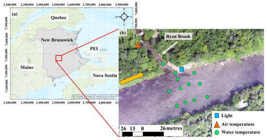
Figure 2.
The Nashwaak River’s location in New Brunswick, Canada (a), and a fine-scale UAV optical image detailing the study site (b). The yellow arrow denotes the river’s flow direction, and the groundwater-dominated tributary “Ryan Brook” is highlighted by the white arrow. Logger locations are indicated by various shapes (see legend).
The study reach was instrumented with an air temperature logger (n = 1), water temperature loggers (n = 12), and a light intensity logger (n = 1) (Figure 2b). The temperature loggers were Onset HOBO UA-002-64 Pendants (±0.53 °C accuracy) and housed in a white uPVC pipe to prevent solar loading. The air temperature logger was placed at ~1.5 m height on a near-by tree, and the water temperature loggers were placed under rocks. Light intensity was also measured with an Onset HOBO UA-002-64 Pendant logger (±10% accuracy). The light logger was placed on a large boulder where it would not be affected by shadows during the study (Figure 2b). Finally, each logger was synchronized to record at 10-min intervals throughout the study period.
2.2. UAV-Based Microbolometer (Zenmuse XT2)
Two DJI Zenmuse XT2 sensors were used in this study. The XT2 is a dual vision sensor comprised of a FLIR Tau 2 thermal sensor and an RGB camera. The thermal imagers are uncooled VOx microbolometers (640 × 512), with a spectral range of 7.5 to 13.5 μm, and noise equivalent differential temperature (NETD) < 50 mk (0.05 °C). The default XT2 sensor has a matte black finish (Figure 3a), and such surfaces have high absorptivity values ~0.95 [47]. To examine the effects of surface absorptivity on UAV-based uncooled microbolometers, one XT2 sensor was retrofitted with reflective polished aluminum foil tape (Figure 3). Polished aluminum has a low absorptivity value ~0.05 [47], and thus should limit temperature increases from solar irradiance on the microbolometer, and provide accurate temperature measurements. The aluminum foil was Nashua© brand heating, ventilation, and air conditioning (HVAC) tape with dimensions of 48 mm × 9 m, and cost CAD$5. The cooling vents of the sensor were not covered to ensure the internal heating and cooling mechanisms of each sensor were identical and comparable (Figure 3c,d). From herein, the black XT2 sensor is referred to as the default sensor (Ds) and the aluminum-shielded XT2 sensor is referred to as the radiation shielded sensor (Rs).
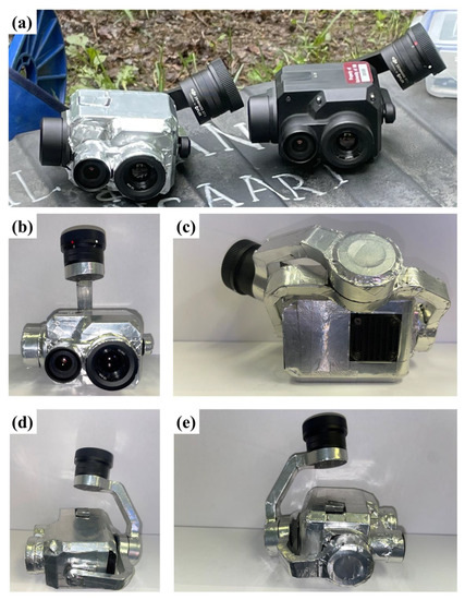
Figure 3.
The two uncooled DJI Zenmuse XT2 sensors are shown in (a) where one sensor is wrapped in aluminum foil tape to provide solar irradiance shielding, and the other is left matte black as per the manufacturer’s default condition. Different viewpoints of the shielded sensor are presented in panels (b–e).
- Flight Plans and Image Processing
Twenty-two flights were conducted over 3 days: n = 6 on 27 June, n = 10 on 29 June, and n = 6 on 30 June 2022. Each flight was preprogrammed using the same flight path (Figure 4) with the DJI Pilot Application, and on average lasted 7 min and 32 s (Table 1). Ref. [48] found the distance between the uncooled TIR sensor and the object of interest affected temperature measurement accuracy. With this in mind, all of the flights in this study were flown at the same height. As per Transport Canada guidelines, the maximum height above ground was set to 124 m. Images were collected at 90% forward overlap and 80% side overlap with the sensor positioned at nadir, as is typical for airborne thermal infrared data acquisition [30]. The resulting flights contained n = 73 TIR and RGB images. The same UAV, a DJI M210 RTK, was used for all data collection. Between each flight the sensors were stored in the shade to reduce any additional heating. A 1500 W generator was also at the site to charge the UAV batteries between flights.
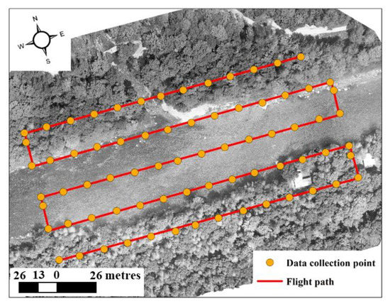
Figure 4.
The flight path for each of the n = 22 flights is shown by the red polyline, and the approximate location of each image collection point is denoted with the yellow dots. Note: these locations can display slight variability under differing wind conditions.

Table 1.
The characteristics of each flight conducted within this study, where Ds is the default sensor surface absorptivity as per the manufacturer, Rs is the modified shielded sensor, and # is the flight number. * For flight 16, the flight was completed quicker than other flights due to a decrease in head wind speed.
The RGB imagery and TIR imagery were processed in Pix4D, with the latter using the Pix 4D thermal image processing module. Typically for TIR image processing the image is corrected for atmospheric conditions which can increase the accuracy of TIR-derived temperature measurements [32,33]. As the main aim of this study was to determine the effect of the sensor’s surface absorptivity on temperature measurement accuracy, the Ds and Rs images were not atmospherically corrected to allow a true sensor treatment comparison. One suite of the TIR images was calibrated with in-stream temperature loggers to visually assess how each sensor’s mosaicked TIR image performed compared to one another and a calibrated TIR image. The calibration model followed a simple multiple linear regression model, where the input parameter was the Pix 4D processed thermal image. This was regressed against data from the in-stream water temperature loggers (Figure 2b).
2.3. Statistical Analyses
Several statistical tests were conducted to (a) assess the accuracy and precision of each sensor and (b) determine the influence of light intensity and air temperature on each sensor’s accuracy. A 2-sample t-test was run if the data were normally distributed, and a Mann–Whitney test was performed if the data were non-normal [30]. For these tests, the input parameter was deviation, which was calculated by subtracting the sensor-derived temperatures from data from the instream temperature loggers (n = 12 for each image). The Ds data and Rs data were grouped separately, resulting in n = 132 comparable data points (12 points per image with 11 images per sensor). Similar to the accuracy analysis, the precision analysis used a 2-sample t-test or a Mann–Whitney test, depending on the distribution of the data. However, to examine precision, the ‘range’ metric was used, which was determined by subtracting the largest deviation from the smallest deviation. This resulted in one range data point per survey, and n = 11 paired samples. In all instances α = 0.05.
To investigate the influence of light intensity and air temperature on the accuracy of sensor-derived temperature measurements, a simple regression approach was used where the parameter of interest, i.e., light intensity or air temperature, was regressed against the average deviation. As the air and light intensity are considered to be spatially constant at the scale of the river reach over the ~7 min for each survey, the deviations described above were averaged for each image; thereby resulting in n = 11 data points for each sensor. Light intensity and air temperature were then individually regressed against the average deviations to investigate the role each had on temperature deviation variability.
3. Results
3.1. Weather Conditions
Both air temperature and light intensity varied over the study period. The 27 June was characterized by altostratus cloud cover, the highest air temperatures (maximum = 25.9 °C; average = 24.5 °C; σ = 0.7 °C), and the lowest light intensity measurements of the study (maximum = 124,000 lux; average = 6225 lux; σ = 3731 lux)—Figure 5a,d,e. The 29 June was predominantly cloud free and had the lowest average air temperatures of the study (maximum = 24.7 °C; average = 21.4 °C; σ = 2.4 °C)—Figure 5b,d. Owing to the clear sky conditions, the light intensity measurements on this day were on average the highest of the study (maximum = 220,445 lux; average = 176,724 lux; σ = 46,470 lux)—Figure 5e. The 30 June was characterized by cumulonimbus and cumulus cloud cover and average air temperature = 21.6 °C (maximum = 22.6 °C; σ = 0.7 °C)—Figure 5c,d. The average light intensity measurement was 115,894 with a maximum of 264,535 lux and σ = 86,774 lux (Figure 5e). A trend between air temperature and light intensity was evident on 29 June; however, no discernable trend was apparent on 27 or 30 June (Figure 5f). A summary of the air temperature and light intensity conditions for each flight is provided in Table 2.
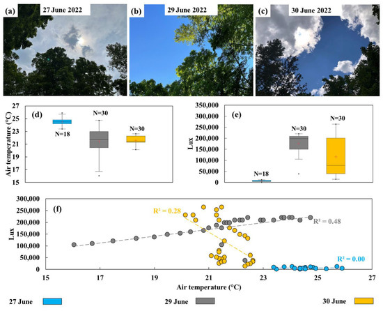
Figure 5.
Cloud conditions during each day are shown in (a–c), and the range of flight specific air temperature and light intensity conditions (measured by lux) for each day are illustrated in (d,e), respectively. The relationship between light intensity and air temperature for each flight reveals no correlation on 7 June, a positive correlation on 29 June, and a negative correlation on 30 June, where the date of data acquisition is denoted by the different colour points (f).
Table 2.
The air temperature (Ta) and light intensity conditions (lux) are provided for each flight, in concert with sensor specific average deviations (Avg. dev. °C) and average deviation ranges (Avg. dev. range °C). The Avg. dev. (sensory accuracy metric) was calculated as the radiant temperature (TR) minus the kinetic temperature (TK) for each flight averaged across the n = 12 instream loggers. The Avg. dev. range is simply the range of Avg. dev. for each flight calculated by TR minus TK and represents sensor precision. # is the flight number.
Light conditions changed during individual surveys at time-steps that were beyond the temporal resolution at which the light loggers were programmed to collect data. An example of this is shown during Flight # 8 (29 June at 10:16) within a 6 s window (Figure 6a,b). In this instance, the light intensity, as observed by the sensor’s RGB camera, is shown to change between 10:20:32 and 10:20:38 even though at this time the UAV is flying in a straight flight path. An illustration of the variability in light conditions between days is also detailed in Figure 6c, where the conditions during Flight # 20 are more muted than those during Flight # 8. This is also apparent in the images’ green band digital number (DN) values (Figure 6d–f), where the DN values are shown to change for the same location under different light conditions at intra- and inter-flight scales.
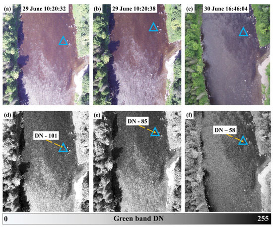
Figure 6.
Light conditions varied at the intra-flight timescale as is shown in (a,b), and also varied at the inter-flight (daily) scale (c)—where all images are from the Rs optical sensor. These changes led to variability in the images’ reflectance, as is shown by the corresponding green band digital number (DN)—(d–f). Here, high DN values denote high reflectance, and thereby low emittance, whilst low DN values detail low reflectance and high emittance. The blue triangles delimit the region where a pixel value was extracted from the green band, and the yellow arrows point to the location of the corresponding DN values shown in (d–f).
3.2. TIR Images from Sensors with High and Low Surface Absorptivity
During data collection immediate differences were apparent between the TIR imagery from the Ds (default) and Rs (aluminum shielded) sensors. The study reach has a dominance of riffles which leads to aerated bubbles (Figure 7a,d). These features were not present in the Ds TIR images (Figure 7b,e). However, the ripples and the associated aerated bubbles were easily identifiable in the Rs TIR images (Figure 7c,f). Even so, the relative thermal heterogeneity was generally consistent in both TIR datasets (see thermal plume extent in Figure 7e,f). The influence of shading on the left bank is spatially consistent between the two TIR datasets (Figure 7b,c). Furthermore, both sensors detected the thermal variability of boulders that are located in full sunlight in contrast with those in the shade (Figure 7a–c).
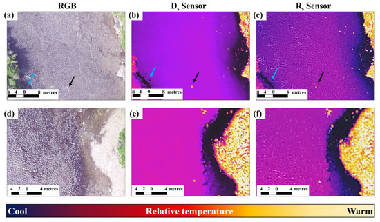
Figure 7.
Qualitatively each sensor (default matte black (Ds) and aluminum shielded (Rs)) detected almost identical patterns of thermal variability. This is evident via the identification of cool boulders located in the shadows (blue arrows), and warm boulders (black arrows) in the open (a–c), and the similarity of the thermal plume extent (d–f). However, the Ds sensor does not detect ripples (b,c), while the Rs sensor does (e,f).
- Sensor Accuracy and Precision Comparison
The comparison of sensor versus instream observed temperature deviations revealed that each sensor displayed thermal drift (Figure 8). It is also apparent that the Ds sensor was prone to greater thermal drift than the Rs sensor (Figure 8d–i). The temperatures derived from the Ds sensor were always lower than the observed temperatures (Figure 8d–f). This cooling offset was also evident for some measurements from the Rs sensor; however, the Rs sensor also had n = 14 temperatures measurements that were higher than the instream observed temperatures. Importantly, the cooling offset was limited on 29 June for both sensors, a day that was characterized by clear sky conditions (Figure 8b). In particular, the surveys that occurred around 10:00 had the lowest range of deviations for both sensors; this time period had relatively low air temperatures (16.0–16.7 °C) and high light intensity (~104,000 to 121,000)—see Table 2.
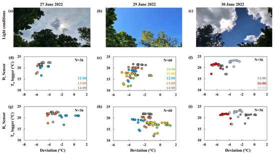
Figure 8.
The cloud conditions are illustrated in (a–c) in concert with the deviation between the instream loggers (Tw n = 12 per flight) and the TIR data from each flight; where panels (d–f) are the deviations for the Ds sensor on 27 June (d), 28 June (e), and 30 June (f), and (g–i) represent the Rs sensors deviations for the same dates, respectively.
Both Ds and Rs deviation datasets were found to be normally distributed where Shapiro–Wilks test results were WDs = 0.98, pDs = 0.06, and WRs = 0.99, pRs = 0.22, respectively. The resulting 2-sample t-test indicated that the deviations between the Ds sensor and the instream temperature loggers (M = −4.3 °C; S.D. = 1.3 °C) were significantly greater than the deviations between the Rs sensor and the instream temperature loggers (M = −2.1 °C; S.D. = 1.6 °C, t(131) = −17.9, p < 0.0001)—Figure 9a.
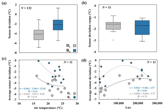
Figure 9.
Sensor deviations for both sensors, with a lower deviation indicating higher accuracy (a). Range of deviations for both sensors (b), with deviation range an indicator of precision. Correlations between sensor deviation and air temperature (c) and sensor deviation and light (d).
The Ds and Rs range datasets were also found to be normally distributed where Shapiro–Wilks test results were WDs = 0.96; pDs = 0.73 and WRs = 0.91; pRs = 0.24, respectively. The resulting 2-sample t-test indicated no significant difference between the Ds sensors range (M = −1.8 °C; S.D. = 0.6 °C) and the Rs sensor and the instream temperature loggers (M = −1.8 °C; S.D. = 0.7 °C, t(10) = 0.64, p = 0.54)—Figure 9b. Thus, these results indicated no statistical difference in the precision of temperatures derived from each sensor.
For both sensors an increase in air temperature was correlated with a decrease in sensor accuracy (defined by sensor deviation) (Figure 9c). The correlation with air temperature was stronger for the Rs sensor than the Ds sensor, R2 = 0.31 and 0.14, respectively (Figure 9c). The direction of the relationship with light intensity was also consistent for the sensors as an increase in light intensity was correlated with an increase in sensor accuracy (Figure 9d). However, the correlation was much stronger for the Ds sensor (R2 = 0.73) compared to the Rs sensor (R2 = 0.40) (Figure 9d). In all instance, a 2nd order polynomial provided the best fit.
The images acquired on 29 June at 10:01 (Ds) and 10:16 (Rs) had the lowest temperature deviations and were consequently chosen as comparative TIR images to access differentials in thermal heterogeneity between images (Table 2; Figure 10a,b). The Rs sensor mosaicked image from 10:16 was chosen to develop a calibrated TIR model to visually compare each sensor’s TIR image accuracy as it had the lowest temperature deviation throughout the study period. The TIR image was calibrated with the instream loggers, and the resulting linear model produced an Adj. R2 = 0.88 and RMSE = 0.7 °C (Figure 10c). The thermal profile defined by the green line in Figure 10a–c is illustrated in Figure 10e and reveals that the Ds sensor largely underestimated the thermal heterogeneity from Ryan Brook to the main river. Although the Rs sensor underestimated the temperature near Ryan Brook, once the profile intersected the main stem, the measurements of the calibrated TIR image and the Rs sensor were indistinguishable (Figure 10e). Of additional interest is the coherence between changes in image brightness (measured from the RGB green band at 0.2 m resolution) and the collocated changes in the temperature measurement errors from each sensor (Figure 10d–f). The brightest areas (measured by the digital number (DN)) are associated with the largest errors, whereas a decrease in DN values leads to a reduction in errors for both sensors (Figure 10e,f).
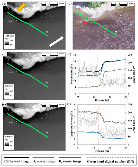
Figure 10.
(a) TIR imagery from flight 8 on 29 June at 10:16 (see Table 2) calibrated with observations from n = 12 instream temperature loggers, where the yellow arrow denotes Ryan Brook, and the white arrow delimits the rivers flow direction. (b) TIR image from the Ds sensor, flight 7 on 29 June at 10:01. (c) TIR imagery from the Rs sensor from flight 8, also used as the calibration image. The RGB image in (d) illustrates the variability of river-bed colour, where the change from Ryan Brook and the main stem is denoted by the red dashed line, and the green profile in (a–d) corresponds with the thermal profiles in (e,f). The different TR measurements from the calibrated image, the Ds sensor, and the Rs sensor are shown in (e), and super-imposed on the corresponding variability in the images’ green band digital number (DN)—a proxy for reflectance—where the red dashed line corresponds to the red dashed line in (d). Temperature measurement errors between the calibrated TIR image and the Ds and Rs TR measurements are shown in (f), where a decrease in DN values leads to a reduction in errors for both sensors.
4. Discussion
In this study we tested three hypotheses: (1) that reduced surface absorptivity of uncooled microbolometers would limit thermal drift, (2) that clear sky conditions would increase the signal-to-noise ratio of the microbolometer thereby limiting thermal drift, and (3) that an increase in air temperature would lead to an increase in thermal drift. The results generally validate our hypotheses and can provide a useful suite of guidelines for increasing the accuracy of uncooled UAV-based TIR temperature measurements. However, prior to that we discuss the key findings of this study.
4.1. The Link between Sensor Surface Absorptivity and Thermal Drift
It is well established that a major limitation of uncooled TIR sensors, herein specifically microbolometric sensors, is they are highly sensitive to temperature changes due to internal heating from the device operation and external heating. Many of the radiometric UAV microbolometric TIR sensors available today are black, e.g., Workswell WIRIS Pro, FLIR Duo Pro R, FLIR Vue Pro R, DJI Zenmuse XT2, DJI Zenmuse H20N, DJI Zenmuse H20T. Black objects have the highest absorptivity values, and this high absorptivity will increase the sensor’s surface temperature due to solar irradiance when left exposed. As the sensor temperature increases, the heat energy radiated from the sensor will increase rapidly as per the Stefan–Boltzmann Law. Theoretically, the increase in radiated heat energy will alter the temperature of the uncooled microbolometer, thereby modifying the electrical resistance the sensor relies on for accurate measurements [4,39,40]. Our results suggest solar irradiance heat energy gains can be somewhat ameliorated by simply wrapping the microbolometric TIR sensor in a polished foil (Figure 2). We found this led to a reduction in thermal error by an average of 2.2 °C compared to the unshielded sensor (Figure 9).
In all instances, the Ds sensor underestimated TK, and generally this underestimation was also apparent in the Rs sensor’s TIR images (Figure 8). However, the Ds sensor’s TR errors were larger than the Rs sensor’s errors. For example, in one flight (30 June ~14:00), the Ds derived TR underestimated TK by ~7 °C compared to ~2 °C for the Rs sensor (Figure 8f,i, respectively). Interestingly, [33] found both positive and negative thermal drifts with the unshielded sensor, at least for the study in the Baddoch Burn in Scotland. However, we did not observe any positive thermal drift in the 11 DS sensor flights. This poses the question: what is driving the substantial negative thermal drift observed in this study? As mentioned earlier, microbolometers operate on the principle of the bolometric effect, where a change in the electrical resistance of a material is caused by temperature increases arising from absorbed radiation in the microbolometric element [38]. The temperature dependence of electrical resistance is computed by the temperature coefficient (β) and is mathematically expressed as [4]:
where R is electrical resistance and T is temperature.
The resulting change in resistance due to an increased temperature (∆T) can be found by:
where is the average value in the temperature interval ∆T. Under steady-state conditions, ∆T is [4]:
where αΦ0 is the absorbed radiation power and Gth is the thermal conductance.
Substituting Equation (3) into Equation (2) yields:
Equations (3) and (4) indicate that as the thermal conductance of the microbolometer increases, the change in resistance decreases. Furthermore, resistance and temperature are directly proportional (Equation (2)). As thermal conductance is directly proportional to temperature, we suggest heat radiating from the sensor surface leads to an increase in the device’s thermal conductance. This in turn leads to a reduction in ∆R and thereby an underestimated TR from each sensor. This mechanism might also explain why the Rs sensor experienced less thermal drift than the Ds sensor; the reflected solar radiation minimized heat gains at the sensor’s surface, thereby limiting (to some degree) increases in the device’s thermal conductance.
This same mechanism may also shed light on why the Rs sensor identifies ripples, whereas the Ds sensor does not. The stipulated lower thermal conductance associated with the Rs sensor may facilitate the detection of more subtle variations of absorbed radiation power and thereby the detection of ripples. Accordingly, we postulate that changing the surface absorptivity of microbolometric TIR sensors would also increase the sensor’s sensitivity.
4.2. Role of Light Conditions and Air Temperature on Thermal Drift
A hypothesis of this study was that an increase in light intensity would lead to a reduction in thermal drift as this would lead to an increase in the LWIR reaching the sensor, and therefore increase the signal-to-noise ratio. This hypothesis runs contrary to the suggestion by [33] that flights conducted during overcast conditions may reduce thermal drift. Although this suggestion is valid in relation to limiting sensor heating (see above) as overcast days limit solar irradiance and are often cooler, the assumption that overcast conditions themselves would improve measurements overlooks the principle that TIR sensors are passive and are measuring LWIR. The results arising from the 22 flights in this study reveal a positive relationship between light intensity and reduced thermal drift (Figure 9). This relationship was true for both sensors; however, the role of light intensity was most pronounced for the Ds sensor for which light intensity explained 73% of the temperature deviation variability. The greater influence of light intensity on the Ds sensor’s thermal drift can be explained by examining Equation (4). If the suggestion that the thermal conductance is greater for the Ds sensor than the Rs sensor (Section 4.2) is valid, then it would stand to reason that an increase in absorbed radiation power (αΦ0) in the Ds sensor would offset the increased thermal conductance, thereby increasing the electrical resistance. However, this offset has limited capacity to mitigate all of the thermal drift induced by external heat gains due to irradiance, and other factors such as air temperature and wind (Figure 9). Even so, Rs sensor lux values > 100,000 can reduce temperature measurement errors to ≤0.5 °C (Table 2). It is worth nothing that light intensity conditions can change rapidly during a flight and this likely impacts the accuracy of the thermal sensors (see Figure 6). Future studies could investigate how including downwelling irradiance sensors might allow for more accurate calibration of UAV microbolometric TIR sensors.
The increase in accuracy due to light intensity was not spatially consistent. In Figure 10e differences between the TR values from the Rs sensor and the calibrated TIR image are indistinguishable in the main river; however, there are relatively large differences between the Rs TR and the calibrated image of the thermal plume and brook. This was surprising as the mouth of the brook, the plume, and the main river have almost identical light exposure (Figure 10d). We suggest this error is not borne from thermal drift; rather it is underpinned by spatial variability in emissivity. A core principle of TIR processing is correction for emissivity using Kirchhoff’s Radiation Law [7]. In simple terms, the law states that good absorbers are good emitters, and good reflectors are poor emitters. It is clear from Figure 10d that the reflectance of the river changes from high to low (measured via the images DN). Higher DNs equate to higher reflectance values, and therefore can be used as a proxy for emissivity variability in this study. The DN of the green band reveals the spatial variability of reflectance due to changes in the river-bed colour, depth, and light attenuation (Figure 10d–f). This change in reflectance tracks the temperature measurement errors in both sensors, where a decrease in reflectance leads to a reduction in the measurement error. Recent work by [49] found the accuracy of a sensor similar to the TIR sensors used in this study increased when emissivity was corrected at the pixel scale. Considering the sensor used in this study has dual TIR and RGB, future studies could examine how such additional processing with paired visual and thermal images could account for fine-resolution variance in emissivity during processing and might alter TIR image accuracy.
Unsurprisingly, air temperature was positively correlated with an increase in sensor deviation. This is consistent with other studies where an increase in air temperature is suggested to increase the temperature of the microbolometer [33]. This increase in sensor temperature would lead to a change in thermal conductance, as described above, thereby inducing thermal drift.
Collating the influence of light conditions and air may explain the parabolic relationship between light intensity and average sensor deviation shown in Figure 9d. For instance, the Rs sensor yielded the lowest temperature deviations when the air temperature was between ~16 and 21 °C and light intensity was >120,000 lux (Table 2; 29 June). We propose that considerations for such environmental variability, in tandem with accounting for surface absorptivity of the sensor and river-bed emissivity, can led to more accurate TIR derived river temperature measurements.
4.3. Relative and Absolute Temperature—Different Tools for Different Questions
Our focus here is addressing challenges with sensing absolute temperatures using UAV-based TIR imagery, but it is important to acknowledge that for many aquatic TIR applications, relative temperatures may be more important. For examples, studies using UAV-based TIR to map locations of thermal refuges for cold-water fish [50], groundwater-dominated tributaries or springs discharging chemically distinct water [25], or urban stormwater contributions [42] may rely only on the thermally anomalous plumes formed at the confluence of thermal disparate waters. Delineating accurate water temperature patterns in space or time may not be important for such mapping exercises that seek to establish relative temperature differences. However, our results still point to the potential to increase the sensitivity of UAV-based TIR imaging by reducing the sensor absorptivity (foil wrapping) or by flying during optimal conditions. Such findings likely have relevance when using UAV-based TIR sensing to quantify riverine thermal heterogeneity [10] or for identifying smaller or less distinct thermal plumes that are collocated with hydrologic inputs of interest [30,51], although such surveys have often been conducted with TIR sensors that are handheld [52] or affixed to piloted aircraft.
4.4. Limitations
This study was limited by other factors that can affect the accuracy and precision of uncooled sensors, such as wind, relative humidity, pitch, roll and yaw of the UAV, and the flight time [33,53]. Additionally, others have found uncooled TIR sensors can benefit from a warming period prior to data collection, and a constant source of heat for sensor calibration [37,54]. However, for UAV studies such steps are difficult as the battery life for most UAV sensors is between 20–35 min, rendering it a difficult trade-off between collecting data and allowing the sensor a warming period. Image processing can also introduce errors that can be carried through to the finalized TIR image. Whilst the air and water temperature data logging intervals for this study are sufficient considering the time of each flight, and in particular the thermal inertia of water, it is now apparent the light intensity logger would be more useful if it was programmed to collect a continuous stream of measurements throughout the entire flight. This would facilitate downwelling corrections and allow a more detailed analysis of how high-temporal resolution variability alters the sensors accuracy.
5. Conclusions
Similar to others [33,37,49], our results demonstrate that thermal drift of uncooled TIR sensors can be substantial. However, our results illustrate the accuracy of UAV-based uncooled TIR measurements can be increased with some simple modifications to the exterior of the sensor, and with considerations for environmental conditions. Accounting for these factors can result in errors in UAV-sensed absolute temperatures that are less than 0.5 °C. The following guidelines for increasing the accuracy of uncooled UAV-based TIR mapping are proposed:
- The exterior absorptivity of the sensor plays a large role in its internal thermal conductance, and an increase in the thermal conductance leads to greater thermal drift. To mitigate this source of thermal drift the sensor should be shielded from solar irradiance using a low absorptivity material, such as polished aluminum tape. This issue could also be remedied by the manufacturer by using a low absorptivity sensor finish. This simple modification also increases the sensor sensitivity; for example, the shielded sensor in this study depicted ripples on the surface of the water, whereas the unshielded sensor did not.
- The accuracy of uncooled TIR sensor measurements depends on light intensity. As TIR sensors are passive, if the goal of data collection is to accurately quantify the temperature of the environment, flights should be flown when the light intensity is >120,000 lux. However, there is a balance between light intensity and air temperature. High light intensity is often associated with high air temperatures, especially during summer. As such, the ideal time for accurate uncooled TIR mapping may be clear-sky conditions with low air temperatures.
- When processing TIR images of waterbodies, it is typical practice to apply the emissivity value of water during image processing. However, our results suggest that changes in emissivity due to river-bed colour, and the associated attenuation of light through the water column, should also be considered. Future work is required to develop more sophisticated methods to delineate the spatial variability of emissivity. These data could then be incorporated into the image processing step, and thereby increase the method accuracy. Additionally, temperature loggers could also be placed in areas with different river-bed colour characteristics. Such practices would aid in developing more accurate calibrated TIR data.
Even with its limitations, the use of UAV-based uncooled TIR sensors will continue to facilitate the development and testing of new conceptual models for understanding thermal variability across a broad range of environments and disciplines, from earth sciences to biotic and ecological sciences.
Author Contributions
A.M.O. conceptualized the study, collected and analyzed the data, and wrote the manuscript with contributions from B.L.K. All authors have read and agreed to the published version of the manuscript.
Funding
Atlantic Salmon Conservation Foundation; Government of New Brunswick, McCain Postdoctoral Fellowship in Innovation, New Brunswick Innovation Foundation, Department of Fisheries and Oceans Canada.
Data Availability Statement
The data for the statistical analyses are provide in the manuscript Tables. Queries regarding these data can be addressed to the corresponding author.
Acknowledgments
The first author would like to thank Lord Pisces, and would also like to thank S. Priestly for help acquiring the 2nd sensor. The authors would also like to thank three anonymous reviewers whose comments helped strengthen this manuscript. Finally, the authors would like to thank M. Richard, A. Pugh, L. Holleran, and A. Morgan for help in collecting these data and the fun days in the field.
Conflicts of Interest
The authors declare no conflict of interest.
References
- Dugdale, S.J.; Klaus, J.; Hannah, D.M. Looking to the Skies: Realising the Combined Potential of Drones and Thermal Infrared Imagery to Advance Hydrological Process Understanding in Headwaters. Water Resour. Res. 2022, 58, e2021WR031168. [Google Scholar] [CrossRef]
- Lee, E.; Yoon, H.; Hyun, S.P.; Burnett, W.C.; Koh, D.C.; Ha, K.; Kim, D.J.; Kim, Y.; Kang, K.M. Unmanned aerial vehicles (UAVs)-based thermal infrared (TIR) mapping, a novel approach to assess groundwater discharge into the coastal zone. Limnol. Oceanogr. Methods 2016, 14, 725–735. [Google Scholar] [CrossRef]
- Bertalan, L.; Holb, I.; Pataki, A.; Szabó, G.; Kupásné Szalóki, A.; Szabó, S. UAV-based multispectral and thermal cameras to predict soil water content—A machine learning approach. Comput. Electron. Agric. 2022, 200, 107262. [Google Scholar] [CrossRef]
- Vollmer, M.; Möllmann, K.P. Infrared Thermal Imaging: Fundamentals, Research and Applications. In Infrared Thermal Imaging: Fundamentals, Research and Applications; Wiley-VCH Verlag GmbH & Co. KGaA: Weinheim, Germany, 2010. [Google Scholar] [CrossRef]
- Scambos, T.A.; Campbell, G.G.; Pope, A.; Haran, T.; Muto, A.; Lazzara, M.; Reijmer, C.H.; van den Broeke, M.R. Ultralow Surface Temperatures in East Antarctica from Satellite Thermal Infrared Mapping: The Coldest Places on Earth. Geophys. Res. Lett. 2018, 45, 6124–6133. [Google Scholar] [CrossRef]
- Handcock, R.N.; Gillespie, A.R.; Cherkauer, K.A.; Kay, J.E.; Burges, S.J.; Kampf, S.K. Accuracy and uncertainty of thermal-infrared remote sensing of stream temperatures at multiple spatial scales. Remote Sens. Environ. 2006, 100, 427–440. [Google Scholar] [CrossRef]
- Handcock, R.N.; Torgersen, C.E.; Cherkauer, K.A.; Gillespie, A.R.; Tockner, K.; Faux, R.N.; Tan, J. Thermal Infrared Remote Sensing of Water Temperature in Riverine Landscapes. In Fluvial Remote Sensing for Science and Management; Wiley: Hoboken, NJ, USA, 2012; pp. 85–113. [Google Scholar] [CrossRef]
- Torgersen, C.E.; Price, D.M.; Li, H.W.; McIntosh, B.A. Multiscale thermal refugia and stream habitat associations of chinook salmon in northeastern Oregon. Ecol. Appl. 1999, 9, 301–319. [Google Scholar] [CrossRef]
- Dugdale, S.J.; Bergeron, N.E.; St-Hilaire, A. Temporal variability of thermal refuges and water temperature patterns in an Atlantic salmon river. Remote Sens. Environ. 2013, 136, 358–373. [Google Scholar] [CrossRef]
- Fullerton, A.H.; Torgersen, C.E.; Lawler, J.J.; Faux, R.N.; Steel, E.A.; Beechie, T.J.; Ebersole, J.L.; Leibowitz, S.G. Rethinking the longitudinal stream temperature paradigm: Region-wide comparison of thermal infrared imagery reveals unexpected complexity of river temperatures. Hydrol. Process. 2015, 29, 4719–4737. [Google Scholar] [CrossRef]
- O’Sullivan, A.M.; Devito, K.J.; Ogilvie, J.; Linnansaari, T.; Pronk, T.; Allard, S.; Curry, R.A. Effects of topographic resolution and geologic setting on spatial statistical river temperature models. Water Resour. Res. 2020, 56, e2020WR028122. [Google Scholar] [CrossRef]
- Casas-Mulet, R.; Pander, J.; Ryu, D.; Stewardson, M.J.; Geist, J. Unmanned Aerial Vehicle (UAV)-Based Thermal Infra-Red (TIR) and Optical Imagery Reveals Multi-Spatial Scale Controls of Cold-Water Areas Over a Groundwater-Dominated Riverscape. Front. Environ. Sci. 2020, 8, 64. [Google Scholar] [CrossRef]
- KarisAllen, J.J.; Kurylyk, B.L. Drone-based characterization of intertidal spring cold-water plume dynamics. Hydrol. Process. 2021, 35, e14258. [Google Scholar] [CrossRef]
- Briggs, M.A.; Hare, D.K. Explicit consideration of preferential groundwater discharges as surface water ecosystem control points. Hydrol. Process. 2018, 32, 2435–2440. [Google Scholar] [CrossRef]
- O’Sullivan, A.M.; Linnansaari, T.; Leavitt, J.; Samways, K.M.; Kurylyk, B.L.; Curry, R.A. The salmon-peloton: Hydraulic habitat shifts of adult Atlantic salmon (Salmo salar) due to behavioural thermoregulation. River Res. Appl. 2021, 38, 107–118. [Google Scholar] [CrossRef]
- Still, C.; Powell, R.; Aubrecht, D.; Kim, Y.; Helliker, B.; Roberts, D.; Richardson, A.D.; Goulden, M.; Still, C.; Powell, R.; et al. Thermal imaging in plant and ecosystem ecology: Applications and challenges. Ecosphere 2019, 10, e02768. [Google Scholar] [CrossRef]
- Goddijn-murphy, L.; Williamson, B.J.; McIlvenny, J.; Corradi, P. Using a UAV Thermal Infrared Camera for Monitoring Floating Marine Plastic Litter. Remote Sens. 2022, 14, 3179. [Google Scholar] [CrossRef]
- Mokhtari, A.; Ahmadi, A.; Daccache, A.; Drechsler, K.; Fritz, S.; Hu, Q.; Jin, Z.; Wu, W.; You, L. Actual Evapotranspiration from UAV Images: A Multi-Sensor Data Fusion Approach. Remote Sens. 2021, 13, 2315. [Google Scholar] [CrossRef]
- Torgersen, C.E.; Faux, R.N.; McIntosh, B.A. Aerial Survey of the upper McKenzie River; Oregon State University: Corvallis, OR, USA, 1999. [Google Scholar]
- Torgersen, C.E.; Faux, R.N.; McIntosh, B.A.; Poage, N.J.; Norton, D.J. Airborne thermal remote sensing for water temperature assessment in rivers and streams. Remote Sens. Environ. 2001, 76, 386–398. [Google Scholar] [CrossRef]
- Monk, W.A.; Wilbur, N.M.; Curry, R.A.; Gagnon, R.; Faux, R.N. Linking landscape variables to cold water refugia in rivers. J. Environ. Manage. 2013, 118, 170–176. [Google Scholar] [CrossRef]
- Dugdale, S.J.; Bergeron, N.E.; St-Hilaire, A. Spatial distribution of thermal refuges analysed in relation to riverscape hydromorphology using airborne thermal infrared imagery. Remote Sens. Environ. 2015, 160, 43–55. [Google Scholar] [CrossRef]
- Wawrzyniak, V.; Piégay, H.; Allemand, P.; Vaudor, L.; Goma, R.; Grandjean, P. Effects of geomorphology and groundwater level on the spatio-temporal variability of riverine cold water patches assessed using thermal infrared (TIR) remote sensing. Remote Sens. Environ. 2016, 175, 337–348. [Google Scholar] [CrossRef]
- O’Sullivan, A.M.; Devito, K.J.; Curry, R.A. The influence of landscape characteristics on the spatial variability of river temperatures. CATENA 2019, 177, 70–83. [Google Scholar] [CrossRef]
- KarisAllen, J.J.; Mohammed, A.A.; Tamborski, J.J.; Jamieson, R.C.; Danielescu, S.; Kurylyk, B.L. Present and future thermal regimes of intertidal groundwater springs in a threatened coastal ecosystem. Hydrol. Earth Syst. Sci. 2022, 26, 4721–4740. [Google Scholar] [CrossRef]
- Frechette, D.M.; Dugdale, S.J.; Dodson, J.J.; Bergeron, N.E. Understanding summertime thermal refuge use by adult Atlantic salmon using remote sensing, river temperature monitoring, and acoustic telemetry. Can. J. Fish. Aquat. Sci. 2018, 75, 1999–2010. [Google Scholar] [CrossRef]
- Wilbur, N.M.; O’Sullivan, A.M.; MacQuarrie, K.T.B.; Linnansaari, T.; Curry, R.A. Characterizing physical habitat preferences and thermal refuge occupancy of brook trout (Salvelinus fontinalis) and Atlantic salmon (Salmo salar) at high river temperatures. River Res. Appl. 2020, 36, 769–783. [Google Scholar] [CrossRef]
- Mejia, F.H.; Torgersen, C.E.; Berntsen, E.K.; Maroney, J.R.; Connor, J.M.; Fullerton, A.H.; Ebersole, J.L.; Lorang, M.S. Longitudinal, Lateral, Vertical, and Temporal Thermal Heterogeneity in a Large Impounded River: Implications for Cold-Water Refuges. Remote Sens. 2020, 12, 1386. [Google Scholar] [CrossRef] [PubMed]
- Fuller, M.R.; Ebersole, J.L.; Detenbeck, N.E.; Labiosa, R.; Leinenbach, P.; Torgersen, C.E. Integrating thermal infrared stream temperature imagery and spatial stream network models to understand natural spatial thermal variability in streams. J. Therm. Biol. 2021, 100, 103028. [Google Scholar] [CrossRef] [PubMed]
- Morgan, A.M.; O’Sullivan, A.M. Cooler, bigger; warmer, smaller: Fine-scale thermal heterogeneity maps age class and species distribution in behaviourally thermoregulating salmonids. River Res. Appl. 2022. [Google Scholar] [CrossRef]
- O’Sullivan, A.M.; Linnansaari, T.; Curry, R.A. Ice Cover Exists (ICE): A quick method to delineate groundwater inputs in running waters for cold and temperate regions. Hydrol. Process. 2019, 33, hyp.13557. [Google Scholar] [CrossRef]
- Wawrzyniak, V.; Piégay, H.; Allemand, P.; Vaudor, L.; Grandjean, P. Prediction of water temperature heterogeneity of braided rivers using very high resolution thermal infrared (TIR) images. Int. J. Remote Sens. 2013, 34, 4812–4831. [Google Scholar] [CrossRef]
- Dugdale, S.J.; Kelleher, C.A.; Malcolm, I.A.; Caldwell, S.; Hannah, D.M. Assessing the potential of drone-based thermal infrared imagery for quantifying river temperature heterogeneity. Hydrol. Process. 2019, 33, 1152–1163. [Google Scholar] [CrossRef]
- Kraaijenbrink, P.D.A.; Shea, J.M.; Litt, M.; Steiner, J.F.; Treichler, D.; Koch, I.; Immerzeel, W.W. Mapping surface temperatures on a debris-covered glacier with an unmanned aerial vehicle. Front. Earth Sci. 2018, 6, 64. [Google Scholar] [CrossRef]
- Mesas-Carrascosa, F.J.; Pérez-Porras, F.; de Larriva, J.E.M.; Frau, C.M.; Agüera-Vega, F.; Carvajal-Ramírez, F.; Martínez-Carricondo, P.; García-Ferrer, A. Drift Correction of Lightweight Microbolometer Thermal Sensors On-Board Unmanned Aerial Vehicles. Remote Sens. 2018, 10, 615. [Google Scholar] [CrossRef]
- Abolt, C.; Caldwell, T.; Wolaver, B.; Pai, H. Unmanned aerial vehicle-based monitoring of groundwater inputs to surface waters using an economical thermal infrared camera. Opt. Eng. 2018, 57, 053113. [Google Scholar] [CrossRef]
- Kelly, J.; Kljun, N.; Olsson, P.O.; Mihai, L.; Liljeblad, B.; Weslien, P.; Klemedtsson, L.; Eklundh, L. Challenges and Best Practices for Deriving Temperature Data from an Uncalibrated UAV Thermal Infrared Camera. Remote Sens. 2019, 11, 567. [Google Scholar] [CrossRef]
- Ostrower, D. Optical Thermal Imaging—Replacing microbolometer technology and achieving universal deployment. III-Vs Rev. 2006, 19, 24–27. [Google Scholar] [CrossRef][Green Version]
- Ravindra, N.M. Microbolometers: Fundamentals, Materials, and Recent Developments; Elsevier: Amsterdam, The Netherlands, 2021; ISBN 9780081028124. [Google Scholar]
- Olbrycht, R.; Wiecek, B.; De Mey, G. Thermal drift compensation method for microbolometer thermal cameras. Appl. Opt. 2012, 51, 1788–1794. [Google Scholar] [CrossRef]
- Briggs, M.A.; Dawson, C.B.; Holmquist-Johnson, C.L.; Williams, K.H.; Lane, J.W. Efficient hydrogeological characterization of remote stream corridors using drones. Hydrol. Process. 2019, 33, 316–319. [Google Scholar] [CrossRef]
- Caldwell, S.H.; Kelleher, C.; Baker, E.A.; Lautz, L.K. Relative information from thermal infrared imagery via unoccupied aerial vehicle informs simulations and spatially-distributed assessments of stream temperature. Sci. Total Environ. 2019, 661, 364–374. [Google Scholar] [CrossRef]
- Anderson, M.P. Heat as a Ground Water Tracer. Ground Water 2005, 43, 951–968. [Google Scholar] [CrossRef]
- Ribeiro-Gomes, K.; Hernández-López, D.; Ortega, J.F.; Ballesteros, R.; Poblete, T.; Moreno, M.A. Uncooled Thermal Camera Calibration and Optimization of the Photogrammetry Process for UAV Applications in Agriculture. Sensors 2017, 17, 2173. [Google Scholar] [CrossRef] [PubMed]
- Furze, S.; O’Sullivan, A.M.; Allard, S.; Pronk, T.; Curry, R.A. A High-Resolution, Random Forest Approach to Mapping Depth-to-Bedrock across Shallow Overburden and Post-Glacial Terrain. Remote Sens. 2021, 13, 4210. [Google Scholar] [CrossRef]
- Rampton, V.N.; Gauthier, R.C.; Thibault, J.; Seaman, A.A. Quaternary Geology of New Brunswick; Geological Survey of Canada: Ottawa, ON, Canada, 1984; p. 5921. ISBN 066011. [Google Scholar]
- Touloukian, Y.S.; Buyco, E.H. Thermophysical Properties of Matter—The TPRC Data Series. Volume 4. Specific Heat—Metallic Elements and Alloys; Thermophysical and Electronic Properties Information Analysis Center: Lafayette, IN, USA, 1971. [Google Scholar]
- Wan, Q.; Brede, B.; Smigaj, M.; Kooistra, L. Factors Influencing Temperature Measurements from Miniaturized Thermal Infrared (TIR) Cameras: A Laboratory-Based Approach. Sensors 2021, 21, 8466. [Google Scholar] [CrossRef] [PubMed]
- Maguire, M.S.; Neale, C.M.U.; Woldt, W.E. Improving Accuracy of Unmanned Aerial System Thermal Infrared Remote Sensing for Use in Energy Balance Models in Agriculture Applications. Remote Sens. 2021, 13, 1635. [Google Scholar] [CrossRef]
- Sullivan, C.J.; Vokoun, J.C.; Helton, A.M.; Briggs, M.A.; Kurylyk, B.L. An ecohydrological typology for thermal refuges in streams and rivers. Ecohydrology 2021, 14, e2295. [Google Scholar] [CrossRef]
- Rosenberry, D.O.; Briggs, M.A.; Delin, G.; Hare, D.K. Combined use of thermal methods and seepage meters to efficiently locate, quantify, and monitor focused groundwater discharge to a sand-bed stream. Water Resour. Res. 2016, 52, 4486–4503. [Google Scholar] [CrossRef]
- Hare, D.K.; Briggs, M.A.; Rosenberry, D.O.; Boutt, D.F.; Lane, J.W. A comparison of thermal infrared to fiber-optic distributed temperature sensing for evaluation of groundwater discharge to surface water. J. Hydrol. 2015, 530, 153–166. [Google Scholar] [CrossRef]
- Aragon, B.; Johansen, K.; Parkes, S.; Malbeteau, Y.; Al-mashharawi, S.; Al-amoudi, T.; Andrade, C.F.; Turner, D.; Lucieer, A.; McCabe, M.F. A Calibration Procedure for Field and UAV-Based Uncooled Thermal Infrared Instruments. Sensors 2020, 20, 3316. [Google Scholar] [CrossRef]
- Virtue, J.; Turner, D.; Williams, G.; Zeliadt, S.; McCabe, M.; Lucieer, A. Thermal Sensor Calibration for Unmanned Aerial Systems Using an External Heated Shutter. Drones 2021, 5, 119. [Google Scholar] [CrossRef]
Publisher’s Note: MDPI stays neutral with regard to jurisdictional claims in published maps and institutional affiliations. |
© 2022 by the authors. Licensee MDPI, Basel, Switzerland. This article is an open access article distributed under the terms and conditions of the Creative Commons Attribution (CC BY) license (https://creativecommons.org/licenses/by/4.0/).