Deep Hash Remote-Sensing Image Retrieval Assisted by Semantic Cues

Abstract

With the significant and rapid growth in the number of remote-sensing images, deep hash methods have become a research topic. The main work of deep hash method is to build a discriminate embedding space through the similarity relation between sample pairs and then map the feature vector into Hamming space for hashing retrieval. We demonstrate that adding a binary classification label as a kind of semantic cue could further improve the retrieval performance. In this work, we propose a new method, which we called deep hashing, based on classification label (DHCL). First, we propose a network architecture, which can classify and retrieve remote-sensing images under a unified framework, and the classification labels are further utilized as the semantic cues to assist in network training. Second, we propose a hash code structure, which can integrate the classification results into the hash-retrieval process to improve accuracy. Finally, we validate the performance of the proposed method on several remote-sensing image datasets and show the superiority of our method.

1. Introduction

With the rapid technological development of remote sensing (RS), the number of remote-sensing images has increased dramatically [1]. Remote-sensing images contain a lot of information, which can be used in agriculture [2], forestry [3], meteorology [4] and other fields. As a result, the need for remote-sensing image processing is also increasing [5,6]. Remote-sensing image retrieval (RSIR) aims to return all images in the dataset that are visually similar to the given query image, which is the fundamental research in many remote-sensing image-processing techniques.

Deep metric learning (DML) is designed to learn similarity measures between data points through deep neural networks. A well-trained DML network can learn an embedding space; in this space, semantically similar samples (the images belong to same class) are close together and dissimilar samples (the images belong to different classes) are far apart [7,8]. Because of its powerful representation capability, DML has been widely applied to various computer vision tasks, including image retrieval [7,8], person reidentification [9,10] and face recognition [11]. However, the feature dimension obtained by DML is always very large, so saving and retrieving these features requires a lot of storage space and computing time. Therefore, hashing methods are combined with DML to generate compact features to improve retrieval speed and save memory space [12]. Hashing algorithms aim to learn a set of hash functions that project the original image from a high-dimensional feature space to a low-dimensional Hamming space, where the intrinsic similarity structure of the image is represented by a binary hash code. Because the similarity of images is effectively measured by the Hamming distance between two hash codes, the hashing algorithm greatly reduces memory consumption and improves retrieval speed. Therefore, the similarity of images can be effectively evaluated on the basis of the Hamming distance of the binary hash codes instead of the Euclidean distance, which is of great importance for large-scale image-processing tasks [13]. The general process of deep hash retrieval is to extract the high-dimensional features of an image by using a deep hash network and then map them to Hamming space by quantization operations to obtain a binary hash code.

Currently, deep metric learning uses only the similarity relationship between samples to learn embedding space. Specifically, deep metric-learning learns the distribution of training samples to build an embedding space by pulling the positive pair closer (increasing the similarity of two samples of the same class) and pushing the negative pair farther apart (decreasing the similarity of two samples of different classes). We define the information utilized in this process as similarity information. In this similarity relationship, we care about only whether the labels of two samples are the same (positive or negative), but do not care about which class each sample specifically belongs to. Equally treating negative samples belonging to different classes does not take full advantage of the information in the label. The classification task requires that the predicted labels match the ground truth of the samples, and in this process, we care not only about whether the samples are of the same class but also about the specific class to which the samples belong. We define this fully exploiting of the labels, which is specific to the classification task but not available in metric learning, as semantic information. We attempt to exploit this semantic information as a cue to assist the retrieval process. In addition, in the hash retrieval process, we would like to incorporate this semantic information into the hash code to achieve better retrieval accuracy. First, metric learning emphasizes bringing samples of the same classes closer together and pushing samples of dissimilar classes farther apart. If the labels are taken into account, the distance between positive samples (from the same class) can be embodied in their similarity hash codes, while the distance between negative samples (from different class) can be increased, which is consistent with the goal of metric learning. Second, metric learning based on the similarity learning strategy focuses only on the distinction between positive and negative samples but does not directly make specific measurement in different negative samples. Adding classes labels can make the final embedding space learn a better distribution by using the distance between labels. We give an example to explain our approach, as shown in Figure 1.

In Figure 1, there are three classes: port, bridge and mountain. Because the two samples in the port class belong to the same class, the distance between the samples is reflected in only the hash code part. The distance between the samples of the port class and the samples of the other two classes is reflected in not only the hash code part but also the binary label code part. This makes the distance between samples belonging to different classes to enlarge, which meets the intrinsic requirements of deep metric learning in that the similar samples should be much closer and in that dissimilar samples should be dispersed.

In summary, we attempt to fully exploit the semantic information of labels to guide the network to learn better representations, and this information can also be used for hash retrieval.

We find that the DML requires that similar samples be clustered together, such that the distribution of samples is too compact in the learned embedding space. In contrast, the classification model needs to learn only the decision boundary between different classes, and the constraint on the distance between similar samples is weaker than that of metric learning such that the distribution of samples in the embedding space is loose. Therefore, we believe that using the semantic information learned from classification labels to assist the metric-learning loss can learn a better embedding space in which the samples have a proper distribution. In fact, we note that some studies have used both the classification loss and the metric-learning loss in the classification domain [14], but there are few similar studies in the retrieval domain. Notably, ref. [15] showed that simply computing the classification loss and the metric-learning loss for the same feature does not improve the performance, because the optimization goals of these two losses are not the same. The metric-learning model may affect the clear decision surface of the classification model, while the classification model may reduce the intraclass compactness of the metric-learning model. Therefore, we need to find an efficient way to combine these two methods and apply them to the retrieval task simultaneously. Out of this consideration, we propose a network architecture, which can classify and retrieve remote-sensing images under a unified framework and which uses classification labels as semantic cues to assist network training for better representation. Figure 2 shows the overall pipeline of the DHCL method.

In addition, we note that in the current approaches, the labels of samples are used only in training and ignored in testing, and we aim to investigate this part further. The retrieval task uses only similarity information to return results, which is consistent with the goal of metric learning, i.e., we do not care about which specific class the given query sample belongs to but rather only about who is closer. We would like to use the labels of the images as a semantic cue in the retrieval process, as a complement to the similarity information. Moreover, how such semantic cues can be combined with hashing methods is also worth investigating. Therefore, we propose a new classification-based hash code encoding scheme. Specifically, we first classify the images then binarize the labels and concatenate them with the hash code. Figure 2 shows how our proposed hash code structure works. When two images are predicted to be similar, the distance between them still depends on the similarity hash code. When two images are predicted to be of different classes, the binary label code can push the distance between them farther apart. In this way, we introduce the classification label as a kind of semantic cue in the retrieval process to make the generated hash code more discriminative.

To demonstrate the effectiveness of our proposed method, we conducted extensive experiments on three commonly used remote-sensing image datasets: UCMD [16] (University of California, Merced, CA, USA dataset), AID [17] (Aerial Image Dataset) and RSD46-WHU [18,19].

The main work and contributions of this paper are as follows:

(1)

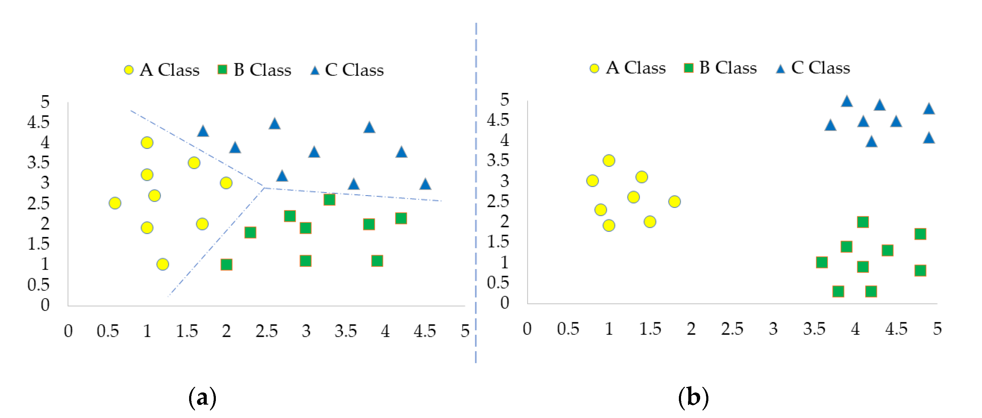
We propose a new deep hash network structure for retrieving and classifying remote-sensing images in a unified framework. This network structure uses semantic information from the classification task to assist in the training of the network, which compensates for the underutilization of label information by previous metric-learning methods and thus improves feature distinctiveness.

(2)

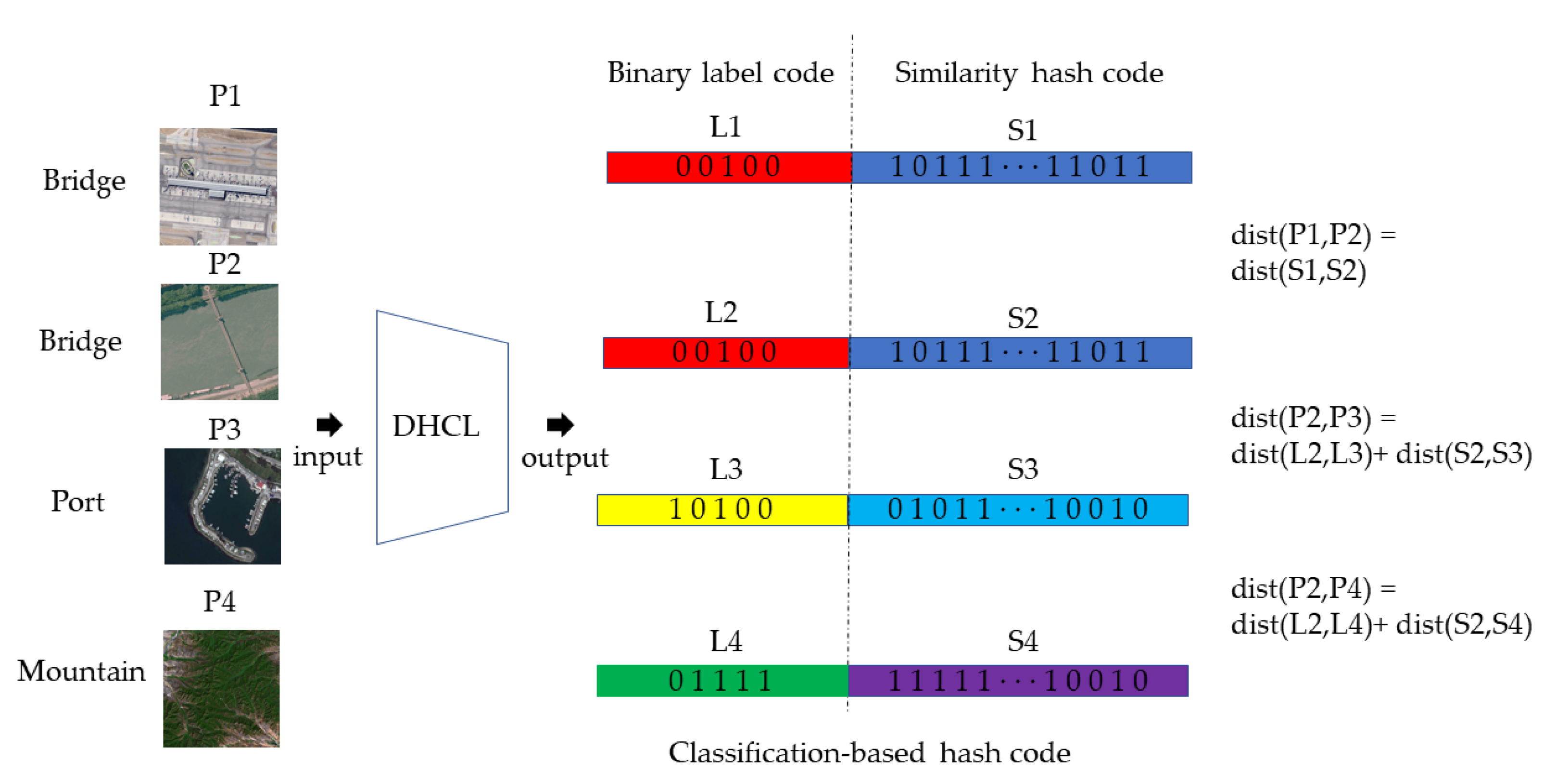
We propose a new hash code structure, which we call a classification-based hash code. This structure can explicitly combine the classification labels with similarity hash codes as a complement in the retrieval process to obtain better ranking relationships.

(3)

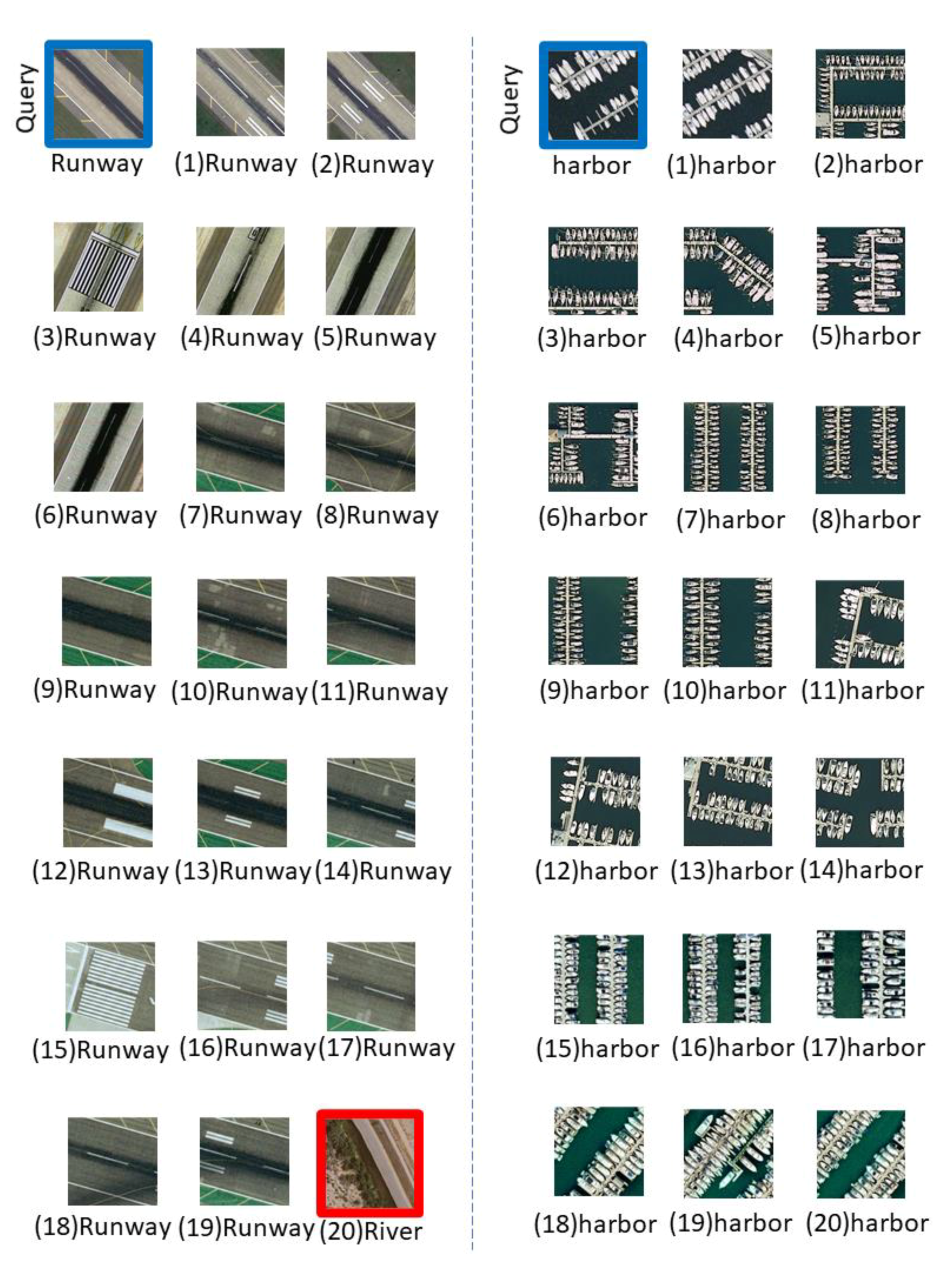
Extensive experiments and comparisons with other methods confirm the effectiveness of our proposed method.

The rest of this paper consists of four parts: Section 2 introduces the related work about deep metric-learning and hashing methods. Section 3 explains our DHCL method. Section 4 lists the experimental results of our DHCL method. Section 5 summarizes the conclusions of our DHCL method.

2. Related Works

2.1. Hashing Method

Because of its speed advantage, hashing methods are widely used as acceleration methods in image retrieval. The goal of hashing methods is to learn a series of hash functions to reduce the dimensionality of features and convert them into a hash code to accomplish the retrieval task. By using manual features or deep features, hashing methods are classified into traditional hashing and deep hashing.

2.1.1. Traditional Hashing Method

Traditional hashing methods usually use manual features such as scale-invariant feature transform (SIFT) [20] or GIST [21]. The kernel-based supervised hashing (KSH) [22] method addresses the linear inseparability problem and uses the labels of the samples to learn highly distinguished hash codes. Iterative quantization (ITQ) [23] method maps centralized sample data onto the vertices of the hypercube, minimizing the quantification error between the rotated data and the hypercube vertex data. However, this manual function usually includes only the content of the picture and is task specific, requiring more specialized experience and manual intervention. The limitations of such methods make it difficult to meet the high-precision requirements of today’s hash retrieval.

2.1.2. Deep Hash Method

Deep hashing methods are based on deep features obtained through convolutional neural networks to learn hash codes and are more discriminative and robust without human intervention. Convolutional neural network hashing (CNNH) [24] is a two-stage hash-learning method. It performs hash code learning and feature learning separately. First, it learns features from pairs of labeled samples and then learns hash codes from the features. Because feature learning and hash code learning are in separate phases, the two information phases in this method cannot optimize each other. The kernel-based supervised locality-sensitive hashing (LSH) method (KSLSH) [25] describes two kernel-based nonlinear hash methods for remote-sensing images. The first hash method uses unlabeled samples to define the hash function. The other describes many unique hash functions by using the semantic similarity extracted from annotated images in the kernel space. Deep pairwise-supervised hashing (DPSH) [26] uses deep features extracted by a CNN, then learns a hash function for high-dimensional feature mapping and finally uses a loss function to measure the quality of the hash code. Each of these steps can provide informative feedback for the optimization of the other steps to accomplish high-performance end-to-end training. The deep hashing neural network (DHNN) [27] method consists of a high-dimensional feature network and a hash neural network, where the neural network is used to extract features and the hash network is for hash mapping. The metric and hash code–learning network (MiLan) [28] method generates hash codes while learning the deep embedding space for efficient hash mapping to accurately represent the semantic information in remote-sensing images and perform real-time retrieval. The deep hashing convolutional neural networks (DHCNN) [12] method redefines image retrieval as both the visual and the semantic retrieval of images. It can complete retrieval and classification at the same time. The method is designed with a loss that takes into account the label loss of each image and the similarity of image pairs. The objective of the deep hashing method is the same as that of DML, so it is possible to combine the deep hashing method with the DML method to obtain better hash-retrieval results.

2.2. Deep Metric Learning

DML aims to learn an embedding space in which similar pairs are close to each other and dissimilar pairs are far from each other, and it is widely used in the field of retrieval [7,8], person reidentification [9,10] and face recognition [11]. DML can be divided into two main categories: pair-based deep metric learning and proxy-based deep metric learning.

2.2.1. Pair-Based Deep Metric Learning

Pair-based losses construct sample pairs from the training set and construct different forms of loss functions according to the diverse sample pairs to achieve optimization goals. Common pair-based loss functions include contrastive loss [29], triplet loss [30], N-pair loss [31], lifted structured loss [32] and multi-similarity loss [33].

Contrastive loss [29] constructs pairs of samples that contain two samples to push the pairs from same class closer and the pairs from different class farther apart. By training, the similarity between positive samples will be improved, while the similarity between negative samples will be reduced and smaller than the threshold.

Triplet loss [30] is a function calculated based on the triplet structure. A triple consists of an anchor point, its positive sample and its negative sample. By optimizing the triplet loss, the similarity between positive sample pairs will be increased and the similarity between negative sample pairs will be reduced. The similarity of positive sample pairs minus the similarity of negative sample pairs is greater than the given margin.

N-pair loss [31] factors in the effect of more samples on the distribution of samples in the embedding space on the basis of triple loss. It gives an anchor and simultaneously selects one sample from the positive class and one from each negative class to assign to the anchor, thus more comprehensively optimizing the sample space.

Lifted structured loss [32] is calculated on the basis of all samples in the training batch. It takes into account all negative samples in the training batch to dynamically construct the most difficult triplet for each positive sample pair. It factors in the effect of more sample relationships in embedding space and therefore provides better assurance of the distribution of features in the embedding space.

Multi-similarity loss [33] analyzes the existing weighting strategies for loss and summarizes three similarity relationships between sample pairs: self-similarity, positive relative similarity and negative relative similarity. Self-similarity is the similarity of a sample to itself directly calculated; positive relative similarity includes the impact of other samples of the same class on the current sample; and negative relative similarity includes the influence of other classes of samples on the current sample. By including the three similarities and introducing hard sample mining, it can more effectively learn embeddings.

By comparing between samples, pair-based loss can provide a rich, supervised signal for the training embedding space by using fine-grained relations. By introducing as many samples as possible into the batch, pair-based losses can exploit more-comprehensive information. However, more samples will result in building more tuples and reduce the convergence speed of the network, whereas selecting too few samples will reduce the training time but may discard some information during training. The training complexity of pair-based losses is $O\left(N^2\right)$ or $O\left(N^3\right)$, where N represents the number of training samples.

2.2.2. Proxy-Based Deep Metric Learning

Proxy-based losses [34,35,36,37] can address the high complexity of pair-based losses. Proxies are initialized to represent a subset of training samples and optimize with the optimization of network parameters. The common idea of proxy-based metric learning is to learn one or more proxies for each class to maintain the global structure of the embedding space, bringing the samples closer to their corresponding proxies and pushing them farther away from other proxies. Unlike the pair-based deep metric learning, proxy-based deep metric learning uses the interaction between data points and proxies instead of sample pair construction, and because the number of proxies is smaller or much smaller than the number of samples, the time complexity of proxy-based methods is less than that of pair-based methods. Currently, the more representative proxy-based losses include proxy-NCA [37] and proxy anchor loss [34].

Proxy-NCA [37] is the earliest proxy-based loss. It generates one proxy for each category in the dataset. The proxy-NCA loss constructs triplets, in which a triplet contains an anchor sample, a positive proxy and a negative proxy. In this way, it associates each sample with all proxies and then brings the similar samples close together and separates dissimilar samples.

Proxy anchor loss [34] is another proxy-based loss. Its benchmark sample is not selected from the training set but rather are proxies constructed from the network parameters. Proxy anchor loss is formulated by associating all samples in the training batch with proxies. Because of the use of proxies, this method can speed up network convergence and fully use global information and the information between samples.

3. Method

This section consists of three parts: Section 3.1 demonstrates the architecture of our DHCL method. Section 3.2 is our loss. Finally, Section 3.3 explains the scheme to generate our classification-based hash code.

3.1. Global Architecture

Deep metric learning pulls the positive pair closer and pushes the negative pair farther away by distinguishing whether the sample points belong to the same class, in which the negative points of different classes are treated equally. However, equally treating negative samples belonging to different classes does not make full use of the information of the labels, and we believe that adding the classification labels as semantic cues can help the network learn better representations. Therefore, in this section, we design a deep hash network structure that can explore both the deep features according to similarity information and the classification features according to semantic information. Figure 2 shows the global architecture of our DHCL method.

The DHCL retrieval system consists of a pretrained CNN, a deep hash network and a full connection layer with a softmax classifier. The labels of input images $\left\{x_1,\cdots ,x_N\right\}$ are processed in one-hot encoding. After encoding, the label of $x_i$ is represented as a vector with length equal to the number of classes in the dataset. In the vector, the position corresponding to the ground truth of $x_i$ is 1 and the other positions are 0. We use $y_i$ to represent the encoded label vector, where $y_i\in T^C$ and $T^C$ represent the true label vectors of the sample $x_i$. C is the total number of classes in the dataset. The corresponding label set is $\left\{y_1,\cdots ,y_N\right\}$. We input the training dataset into the CNN and compute the high-dimensional deep features $\left\{r_1,\cdots ,r_N\right\}$ through a nonlinear transformation $r_i=f\left(x_i;\omega \right)$, where $f\left(·\right)$ denotes the high-dimensional embedding and the $\omega$ represents the parameters of the CNN, which is gradually optimized with the training of the network. Then the high-dimensional deep features are computed using the deep hash network to obtain the low-dimensional hash-like features. It can be denoted as $u_i=tanh\left(r_i;\varpi \right)$, where $\varpi$ is the parameter of the deep hash network. Unlike the training phase, during test phase, the similarity hash codes are calculated by the formula of $b_i=sgn\left(u_i\right)$, which is based on the hash-like feature. To further improve the capability of feature representation, after the deep hash layer, the full connection layer with softmax classifier is used to calculate the class probability distribution of the image. Its calculation formula is $p_i=softmax\left(u_i;\epsilon \right)$, where $\epsilon$ is the parameter of the full connection layer.

3.2. Loss Function

In order to use the semantic information in the classification labels to assist in the training and the hash retrieval, a good classifier is needed. So after the classification layer, the classification cross-entropy loss is calculated to reduce the gap between the predicted class label and the true label. The calculation formula is as follows:

$$L_1=-\frac{{{\displaystyle \sum }}_{i=1}^N⟨y_i,log\left(p_i\right)⟩}{N}, i=1,\cdots ,N$$

(1)

where $y_i$ represents the vector in one-hot encoding of the true label of $x_i$ and $p_i$ represents the probability vector of $x_i$ generated by the classifier. Following a softmax layer, the greatest value of $p_i$ can be denoted as the predicted class. $⟨·⟩$ represents an inner product operation, and N represents the number of input images. Classification loss can monitor the classification accuracy of only a single image; it cannot control the distribution of similarity between images [38] (cannot distinguish between different hash-like features).

Figure 3 demonstrates that the optimized network with classification loss can clearly distinguish between different classes of images, but the distance between different classes of images and the boundary is small, and the distribution between similar images in embedding space is also discrete. However, learned by metric learning, the samples of the positive class are clustered together, whereas the samples of the negative class are farther away.

In last section, we obtained $u_i$, which is the low-dimensional hash-like feature; then we used a proxy-based loss that was proposed in our previous work [39], to calculate the loss of all samples in the training batch. It can be calculated by

$$\begin{gathered} L_{p-loss}=\frac{1}{\left|P^{+}\right|}{\displaystyle \sum }_{i=1}^{\left|P^{+}\right|}log\left(1+{\displaystyle \sum }_{x\in X_P^{+}}{e}^{-{\alpha }_p\left(v_p^i-{\delta }_p\right)}\right) \\ +\frac{1}{\left|P\right|}{\displaystyle \sum }_{i=1}^{\left|P\right|}log\left(1+{\displaystyle \sum }_{x\in X_P^{-}}{e}^{{\alpha }_n\left(v_n^i-{\delta }_n\right)}\right) \end{gathered}$$

(2)

$L_{p-loss}$ is based on proxy anchor loss [34]. Proxy Anchor loss assigns a proxy to each class and uses the proxy to represent the entire class. This method trains the network with sample-proxy association to learn the class features, thus generating a discriminative embedding space. Thanks to the use of sample-proxy association instead of sample-sample association, this method reduces the training complexity from $O\left(n\ast n\right)$ to $O\left(n\ast m\right)$, where $n$ is the number of samples and $m$ is the number of classes. In general, $m$ is much smaller than $n$, so this kind of method has lower time complexity. In Equation (2), $P$ represents all proxies, and the proxy corresponding to the class in current batch is called positive proxy $P^{+}$. In the training process, each positive proxy will be specified as an anchor, and the samples of the same class as the anchor are positive samples $x\in X_P^{+}$, and the other samples are negative samples $x\in X_P^{-}$. $v_p^i$ represents the cosine similarity between $u_i$ and its positive proxy, and $v_n^i$ represents the cosine similarity between $u_i$ and its negative proxy.

On this basis, we use a dynamic strategy to mine the relationship between samples. Specifically, ${\alpha }_p=max\left(0, O_p-v_p\right)$ and ${\alpha }_n=max\left(0, v_p-O_n\right)$ are adaptive parameters that can be learned during the training process. $O_p$ is the best similarity between the positive sample and an anchor. $O_n$ is the optimal similarity between the negative sample and anchor. We set them to $1+m$ and $-1-m$, respectively. By adjusting ${\alpha }_p$ and ${\alpha }_n$, the optimization direction of positive and negative samples can be controlled. ${\delta }_p$ and ${\delta }_n$ are the margin of the positive pairs and the negative pairs, respectively, where the margin controls the degree of dispersion between samples. In addition, we set them to $1-m$ and $-1+m$, respectively. $m$ is a hyperparameter to control the dynamic strategy.

Significantly, the features learned through the above loss function will lose information in the process of quantization into hash code. In addition, the existence of discrete values makes derivative calculation difficult. Therefore, before quantifying, the similarity score is calculated. However, we also need to minimize the loss in the process of quantifying hash-like features into hash codes, so we introduce quantification loss:

$$L_{b-loss}={\displaystyle \sum }_{i=1}^N{\parallel u_K^i-b_K^i\parallel }_2^2$$

(3)

where K denotes the length of the hash code, N denotes the number of input images, $u_K^i$ is the i-th hash-like feature and $b_K^i$ is the i-th similarity hash code. The similarity has code is derived from a formula: $b_K=sgn\left(u_K\right)$, which quantifies the hash-like feature. $sgn\left(·\right)$ is a symbol function that returns the positive and negative symbols of a variable: 1 for positive values and −1 for negative values. ${\parallel ·\parallel }_2^2$ means the $l_2$ norm vector, which is used to reduce the distance between the similarity hash codes and the hash-like features. The final metric learning loss is as follows:

$$L_2=L_{p-loss}+L_{b-loss}$$

(4)

By minimizing $L_2$, the feature distances between similar samples are reduced, whereas those between different samples are enlarged.

In summary, $L_2$ is designed to learn similarity information between images, and $L_1$ is designed to learn semantic information for each image. Therefore, we combine the above two losses to obtain the final loss. The specific form of the function is as follows:

$$L_3=\eta L_1+\left(1-\eta \right)L_2$$

(5)

We use a parameter $\eta \in \left[0,1\right]$ to balance semantic and similarity information. Specifically, when $\eta =1$, the loss uses only the semantic information of each image, and when $\eta =0$, the loss uses only the similarity information between images.

The AdamW optimizer [40] is used to optimize our DHCL method, and the optimization process is show in Algorithm 1.

Algorithm 1: Optimization algorithm of our proposed DHCL method.

Input:

A batch of remote-sensing images.

Output:

The network parameter W of the DHCL method.

Initialization:

Random initialize parameter W.

Repeat:

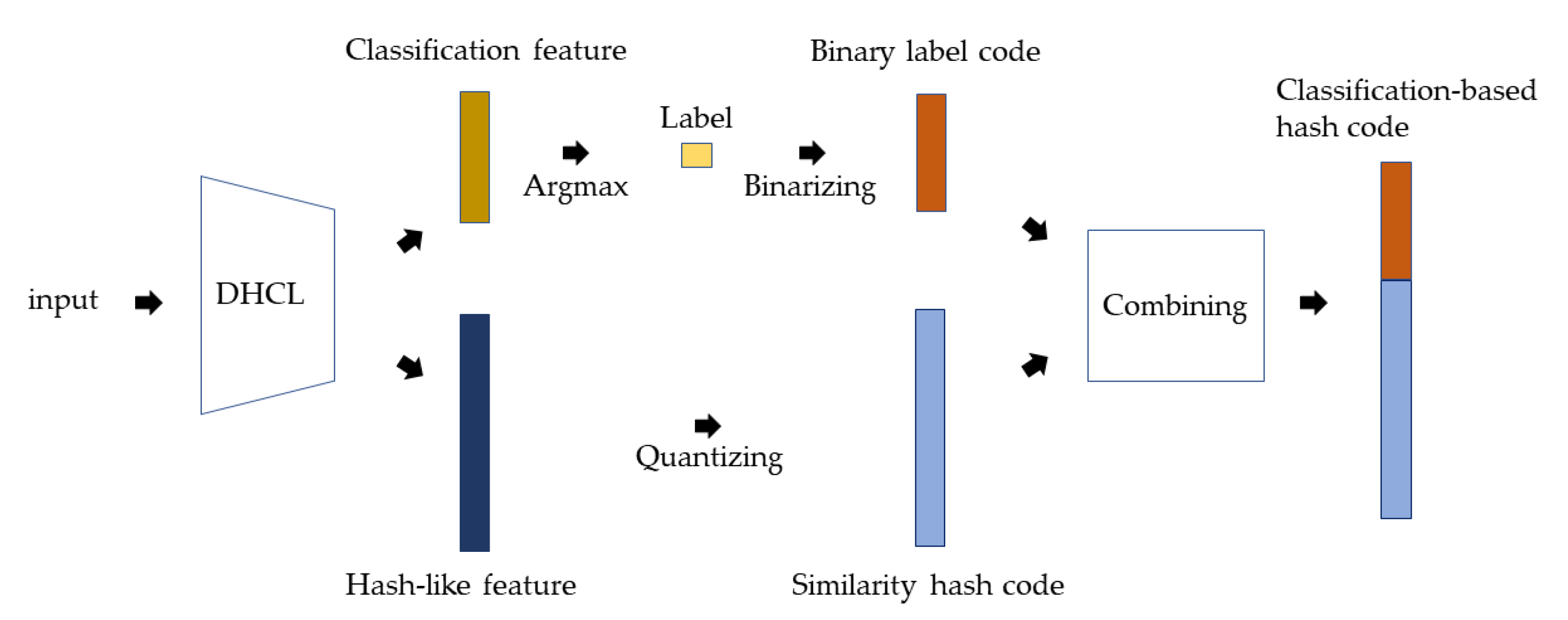
1: Compute hash-like feature $u_i$ and classification label feature $p_i$ by forward propagation;

2: Compute similarity hash code $b_K^i$ by $sgn\left(·\right)$;  3: Utilize $p_i$, $u_i$ $b_K^i$ to calculate loss according to Equation (5);

4: Use AdamW optimizer to recalculate W.

Until:

A stopping criterion is satisfied

Return: W.

3.3. Hash Code Generation

Because the training phase trains the network parameters by using semantic information and similarity information, a well-trained network can be used to generate predicted labels and the low-dimensional hash-like features of images, respectively. Binary label codes and similarity hash codes can be generated by the binary processing of class labels and the quantification of low-dimensional hash-like features. By combining the two binary codes, the final hash code can be generated, which can be used for efficient and high-precision retrieval. The generation of final hash codes is shown in Figure 4.

As in Figure 4, during the test phase, when we obtain $p_i$, which is the predicted probability distribution vector of length C, we can use the formula $c_i=argmax\left(p_i\right)$ to obtain the prediction label for the current image. The binary label code is obtained by binary representation of $c_i$, which is the prediction label, and its length is $lo{g}_{2}C$. The hash code for saving the visual content of the image itself is through the formula of $b_i=sgn\left(u_i\right)$, and it has the same length as $u_i$, which is $K-lo{g}_{2}C$, where K denotes the size of the hash code. The final classification-based hash code is generated by combining $c_i$ and $b_i.$ One part of the classification-based hash code is used to save the semantic information, and the other part is used to save the similarity information of the image. The length of the $c_i$ is very small, so the hash code structure in this section can be consistent with the length of 16, 32, 48 and 64 bits commonly used in hash retrieval, which also avoids the additional consumption of time or space.

4. Experiments

Section 4 consists of six parts: Section 4.1 introduces the datasets and evaluation criteria that we used. Our implementation details are in Section 4.2. Section 4.3, Section 4.4 and Section 4.5 detail, respectively, our experiment results on UCMD, AID and RSD46-WHU; our ablation experiment; and our classification results. Finally, Section 4.6 discusses our findings.

4.1. Dataset and Criteria

We use UCMD, AID and RSD46-WHU datasets to verify the effectiveness of our DHCL method. The full name of UCMD [16] is University of California, Merced, CA, USA dataset. The dataset has 21 classes, and each class consists of 100 surface images with 256 × 256 pixels and 0.3 m spatial resolution. The AID [17] (aerial image dataset) has 30 classes, 10,000 images in total, of which the pixel size is 600 × 600. The RSD46-WHU [18,19] is a large-scale remote-sensing dataset, which contains 117,000 images with 46 classes, and each class contains 500–3000 images. In these datasets, images from the same class can be considered as ground-truth neighbors.

We use mAP (mean average precision) as the evaluation criterion to compare the effects of different retrieval methods, which can be calculated by

$$\mathrm{mAP}=\frac{1}{\left|Q\right|}{\displaystyle \sum }_{i=1}^{\left|Q\right|}\frac{1}{n_i}{\displaystyle \sum }_{j=1}^{n_i}precision\left(R_i^j\right)$$

(6)

where |Q| is the size of the testing set, $R_i^j$ is the j-th retrieval image acquire from the i-th test sample, $R_i$ is the set of $R_i^j$ and $n_i$ is the size of $R_i$.

4.2. Implementation Details

We use Inception Net [41] pretrained on ImageNet [42] as our backbone. We use remote-sensing datasets and our designed loss to fine-tune the parameters of the backbone during training. The AdamW optimizer [40] is used, and the initial learning rate is 0.0001. Training samples are randomly selected, and the batch size is 90. The proportions of the training set and the test set of UCMD and AID are 8:2 and 5:5, respectively. For RSD46-WHU, we use 85 percent of all images as the training set and the rest as the test set. We set the value of $\eta$ to 0.2.

4.3. Experimental Results

In this section, we present the experimental data for UCMD and AID. The results on UCMD and AID are analyzed to explain the effect of our DHCL method. Figure 5 and Figure 6 preliminarily show an example of our retrieval results on UCMD and AID. Section 4.3.1 and Section 4.3.2 discuss the findings of our method and its comparison with other methods in conjunction with specific data. Section 4.3.1 is the results on UCMD. Section 4.3.2 is the results on AID. Finally, in Section 4.3.3, we evaluate the retrieval speed on RSD46-WHU.

4.3.1. Results on UCMD

We compare the latest deep hash methods with our DHCL method, including DHPL [39], DHCNN [12], DHNN-L2 [27], DPSH [26], KSH [22], ITQ [23], SELVE [43], DSH [44] and SH [45] to verify the effectiveness. DHPL is a deep hashing method using proxy-based loss. DHCNN, DHNN-L2 and DPSH are deep hashing methods using a contrastive loss-like hash feature–generation mechanism, and KSH, ITQ, SELVE, DSH and SH are traditional hashing methods. The first 80 images of each class in the UCMD dataset are used for training and the remaining 20 images for testing. We choose four commonly used hash code lengths for our experiments.

Table 1. Results of different retrieval methods on UCMD. The latest hash methods, including DHPL, DHCNN, DHNN-L2 and DPSH, and KSH, ITQ, SELVE, DSH and SH are compared with our DHCL method. The respective lengths of the hash codes used for retrieval are set to 16 bits, 32 bits, 48 bits and 64 bits.

Method	Hash Code Length
	16 Bits	32 Bits	48 Bits	64 Bits
DHCL	98.97	99.34	99.54	99.60
DHPL [39]	98.53	98.83	99.01	99.21
DHCNN [12]	96.52	96.98	97.46	98.02
DHNN-L2 [27]	67.73	78.23	82.43	85.59
DPSH [26]	53.64	59.33	62.17	65.21
KSH [22]	75.50	83.62	86.55	87.22
ITQ [23]	42.65	45.63	47.21	47.64
SELVE [43]	36.12	40.36	40.38	38.58
DSH [44]	28.82	33.07	33.15	34.59
SH [45]	29.52	30.08	30.37	29.31

lists the results of different traditional hash-retrieval methods, deep hash methods and our DHCL method, and the evaluation standard is mAP.

Table 1 shows that our DHCL method is capable of obtaining better results in the retrieval of different hash code lengths on UCMD. Under the assumption that the hash code length is 16 bits, our DHCL approach outperforms the DHPL method by 0.44 (from 98.53 to 98.97) and the DHCNN method by 2.45 (from 96.52 to 98.97). While the hash code length is increased to 32 bits, the retrieval result of our DHCL method is 0.51 (from 98.83 to 99.34) higher than that in the DHPL method and 2.36 (from 96.98 to 99.34) higher than that in DHCNN. Our method surpasses DHPL and DHCNN by 0.53 (from 99.01 to 99.54) and 2.08 (from 97.46 to 99.54), respectively, when the hash code length is increased to 48 bits. When the hash code length is 64 bits, our DHCL approach outperforms the DHPL method by 0.39 (from 99.21 to 99.60) and the DHCNN method by 1.58 (from 98.02 to 99.60).

We find that for all methods, the mAP increases as the hash code length grows, but it is not significant. This is because UCMD is a simple dataset and because the shorter hash codes are sufficient to contain the information. However, the mAP for DHCL with respect to all hash code lengths stays highest above other methods. This indicates that our DHCL method learns a discriminative embedding space and efficiently maps the embedding vector to the Hamming space. In addition, classification-based hash code strategy can effectively improve retrieval performance.

4.3.2. Results on AID

We then conduct an evaluation on the AID dataset, the methods used for comparison still include DHPL [39], DHCNN [12], DHNN-L2 [27], DPSH [26], KSH [22], ITQ [23], SELVE [43], DSH [44] and SH [45]. During the experiment, 50% of the images in each class are used for training, and the remaining images are used for testing.

Table 2. Results of different retrieval methods on AID. The latest hash methods, including DHPL, DHCNN, DHNN-L2, DPSH, KSH, ITQ, SELVE, DSH and SH, are compared with our DHCL method. The respective lengths of the hash codes used for retrieval are set to 16 bits, 32 bits, 48 bits and 64 bits.

Method	Hash Code Length
	16 Bits	32 Bits	48 Bits	64 Bits
DHCL	94.75	98.08	98.93	99.02
DHPL [39]	93.53	97.36	98.28	98.54
DHCNN [12]	89.05	92.97	94.21	94.27
DHNN-L2 [27]	57.87	70.36	73.98	77.20
DPSH [26]	28.92	35.30	37.84	40.78
KSH [22]	48.26	58.15	61.59	63.26
ITQ [23]	23.35	27.31	28.79	29.99
SELVE [43]	34.58	37.87	39.09	36.81
DSH [44]	16.05	18.08	19.36	19.72
SH [45]	12.69	16.99	16.16	16.21

lists the results.

Experiment findings suggest that our DHCL approach produces the greatest outcomes under different hash code lengths on the aid dataset. When the hash code gradually increases from 16 bits to 64 bits, the DHCL method is 1.22 (from 93.53 to 94.75), 0.72 (from 97.36 to 98.08), 0.65 (from 98.28 to 98.93) and 0.48 (from 98.54 to 99.02) higher than the DHPL method, respectively. In addition, the DHCL method is 5.7 (from 89.05 to 94.75), 5.11 (from 92.97 to 98.08), 4.72 (from 94.21 to 98.93) and 4.75 (from 94.27 to 99.02) higher than the DHCNN method, respectively.

For the more complex AID dataset, as the hash code grows from 16 bits to 32 bits, the different methods all show a large improvement. This shows that the 16-bit hash code does not accommodate the information contained in the data well. However, when the hash code was increased from 32 bits, the growth of the retrieval results slowed down. Therefore, we believe that the 32-bit hash code is the optimal choice, which can well balance retrieval accuracy and the requirements. On this dataset, DHCL method achieves a greater improvement than on the UCMD dataset. This indicates that adding semantic information as a cue can boost the network’s training and learning in a more discriminative embedding space.

4.3.3. Results on RSD46-WHU

On UCMD and AID, we evaluated the effectiveness of DHCL. In addition, we use RSD46-WHU, which is a large-scale remote-sensing dataset to validate the retrieval speed. We use 85% of the images in each class for training, and the other for testing. To achieve more comprehensiveness, we select two methods: one is retrieval in Hamming space, and the other is retrieval in Euclidean space. DHPL [39] is the same deep hash method as the proposed method without our classification-based hash code strategy. In addition, VDCC [19] is a nonhash method. However, VDCC also uses a dimensionality reduction strategy to compress the deep features. For fairness, the hash codes and features are of the same length and set to 16, 32, 48 and 64, respectively, for comparison experiments. The evaluation criterion for retrieval accuracy is mAP. In addition, the average retrieval time is used to evaluate speed.

Table 3. Results of different retrieval methods on RSD46-WHU. The respectively lengths of the hash codes and features are set as 16 bits, 32 bits, 48 bits and 64 bits. The evaluation criterion for retrieval accuracy is mAP. Finally, the evaluation criterion for time is the average retrieval time, in milliseconds.

Method	Hash Code or Feature Length
	16 Bits		32 Bits		48 Bits		64 Bits
	mAP	Time (ms)	mAP	Time (ms)	mAP	Time (ms)	mAP	Time (ms)
DHCL (Hamming)	90.87	848.9	94.61	859.0	95.03	865.8	95.38	869.2
DHCL (Euclidean)	92.26	1179.2	95.05	1202.6	95.25	1212.8	95.60	1226.4
DHPL [39] (Hamming)	89.94	848.9	92.58	859.2	93.67	865.8	94.05	869.2
DHPL [39] (Euclidean)	91.34	1179.4	93.38	1202.6	93.72	1212.7	94.27	1226.5
VDCC [19] (Euclidean)	54.25	1179.2	60.30	1202.5	62.78	1212.7	66.59	1226.4

shows that DHCL outperforms DHPL by 0.93 (from 89.94 to 90.87), 2.03 (from 92.58 to 94.61), 1.36 (from 93.67 to 95.03) and 1.13 (from 94.05 to 95.38) when the hash code length is 16 bits, 32 bits, 48 bits and 64 bits, respectively, in retrieval accuracy. Because the DHPL of equal length does not introduce a class label and uses only metric loss to generate hash-like codes, this demonstrates that the introduction of class labels can to some extent improve the distinguishability of feature representations. In addition, we compare the retrieval result in Euclidean space. The DHCL method in Euclidean space is 0.92 (from 91.34 to 92.26), 1.67 (from 93.38 to 95.05), 1.53 (from 93.72 to 95.25) and 1.33 (from 94.27 to 95.60), respectively, higher than DHPL in Euclidean space. We also compare it with VDCC, which uses a dimensionality reduction strategy to compress the deep features. In addition, DHCL is 38.01 (from 54.25 to 92.26), 34.75 (from 60.30 to 95.05), 32.47 (from 62.78 to 95.25) and 29.01 (from 66.59 to 95.60), respectively, higher than VDCC. Our DHCL still achieves better retrieval accuracy than the other two methods in the Euclidean space. This demonstrates that our DHCL method can guarantee high retrieval accuracy while maintaining the retrieval speed of the hash method.

4.4. Ablation Study

To select the most appropriate hyperparameter $\eta$, the ablation experiments on UCMD datasets are performed to validate the values. During the experiment, we explore the results of gradually increasing the value of $\eta$ from 0.0 to 1.0 in 0.2 steps with different hash code lengths. Figure 7 shows the results of ablation experiments in the form of a bar chart.

In Figure 7, we can perceive that the longer the hash code, the higher the precision of retrieval. Meanwhile, when $\eta$ is 1 (training the network with classification loss only), we obtain the worst results because the classification loss aims to draw a clear decision boundary between different classes and does not maintain a compact distribution relation of samples in the embedding space, which is consistent with our conclusion in Figure 3. We obtain the second lowest result when $\eta$ is 0 (training the network with only metric learning loss), which shows that adding classification labels as semantic cues can assist the network in learning better representation, and because our hash code consists of binary label codes and similarity hash codes concatenated together, losing the accuracy of either aspect can lead to a decrease in retrieval accuracy. The retrieval accuracy reaches the highest when $\eta$ is equal to 0.2. Therefore, we set the value of $\eta$ to 0.2 in the subsequent experiments.

We evaluate the impact of classification loss and classification labels on retrieval performance. In fact, the feature extraction of the main network has been affected during the training process after the classification loss has been added, but we want to further determine whether the explicit introduction of binary label codes in the testing process will even more improve the experimental results. Therefore, we set up a set of comparative experiments under the conditions of introducing classification loss and a binary label code, introducing classification loss without a binary label code and introducing a binary label code on the basis of metric-learning loss without classification loss.

Table 4. Settings of evaluation experiment. Method 1 is DHCL. Method 2 uses classification loss and metric-learning loss, but only similarity hash codes are used in the retrieval process. Method 3 uses only metric-learning loss and uses labeled binary codes and similarity hash codes in the retrieval process.

Method	Training		Testing
	Training Loss		Hash Code
	Classification Loss	Metric-Learning Loss	Binary Label Code	Similarity Hash Code
Method 1 (DHCL)	√	√	√	√
Method 2	√	√		√
Method 3		√	√	√

shows the settings of our evaluation experiment. Method 1 uses both classification loss and metric-learning loss in the training process and binary label codes and similarity hash codes in the test phase; method 2 uses both classification loss and metric-learning loss in the training process but only similarity hash codes in the test phase; and method 3 uses metric-learning loss in the training process and binary label codes and similarity hash codes in the test phase.

Table 5. Results of evaluation experiment on UCMD. DHCL achieved the best result, followed by method 2, and method 3 achieved the worst result.

Method	Hash Code Length
	16 Bits	32 Bits	48 Bits	64 Bits
Method 1(DHCL)	98.97	99.34	99.54	99.60
Method 2	98.42	98.54	99.46	99.53
Method 3	85.30	86.40	86.93	87.02

shows our experimental results on UCMD, in which the methods correspond to the settings in Table 4. From Table 5, we can see that whether the hash code length is 16 bits, 32 bits, 48 bits or 64 bits, method 1 has a small improvement over method 2, and the results of method 1 and method 2 are much higher than those of method 3. In this way, we can say the introduction of classification loss in training can help the network learn the appropriate features, which plays the most important role in the whole architecture. At the same time, the explicit introduction of binary label codes can further improve the retrieval effect on that basis. The reason for this effect is shown in Figure 1. Samples predicted to be of the same class have the same binary label code and have no effect on the distance in Hamming space, while samples predicted to be of different classes have different binary label codes, which will increase the distance in Hamming space and thus can help to push samples of different classes away.

4.5. Results on Classification

As our method can obtain the result of the classification label of the input image, the retrieval system can complete the classification task at the same time. Therefore, the classification experiments of UCMD and AID are carried out in order to test the efficiency of the deep hash-retrieval system on the basis of classification labels in classification. DHCNN, SPP [46], MSP [47], DCA [48] and GBRCN [49] are used for comparison.

Similar to the DHCNN method, 80% of the samples in the UCMD and 50% of the AID are randomly selected for training, whereas the remainder of the samples are utilized to assess classification performance. We set the hash code length to 64 bits. The overall accuracy (OA) is used as the index to evaluate classification performance, which refers to the ratio between the quantity of correct images predicted on all test sets and the total number of test samples.

Figure 8 shows that our method can not only complete the classification task but also achieve the highest classification accuracy on UCMD and AID.

4.6. Discussion

According to the above test results, we find that our DHCL method achieves the best performance on UCMD, AID and RSD46-WHU. Our method proposes improvements from both training and testing phases. During training, our method used both classification loss and proxy-based metric-learning loss, which not only learns the proper distribution of samples in the embedding space but also reduces the training complexity.

Meanwhile, the experimental results are consistent with our proposed theory that the distribution of samples in the embedding space is not well maintained when only classification loss is used but can help the network learn a better distribution by adding semantic information from the classification process with appropriate strength. We find that the optimal ratio of metric-learning loss to classification loss is 4 to 1. When this ratio increases, the samples in the embedding space are too compact, whereas when this ratio decreases, the samples in the embedding are too dispersed. However, when the hash code length is large enough, adding classification labels is not completely meaningless.

In addition, during testing, we found that explicitly introducing binary label codes can further improve the accuracy of r-retrieval. This has no effect on samples from the same class, but it helps to push samples from different classes apart. This improvement is more pronounced when the hash codes are short, probably because shorter hash codes are not sufficient to accurately characterize the images, and thus, label information can provide greater assistance. In addition, longer hash codes can store more information and bring better retrieval results, whereas shorter hash codes have poorer retrieval results. However, from the perspective of retrieval, longer hash codes imply higher requirements for memory space and retrieval time. To balance the accuracy and time consumption of remote-sensing image retrieval, we find that 32 bits can guarantee the performance at an acceptable cost.

5. Conclusions

In this paper, we observed that the metric-learning method cared about only whether two samples belonged to the same class and equally treated samples of different classes, which led to insufficient utilization of the semantic information in the labels. Therefore, we used classification methods as semantic cues to assist metric-learning methods in order to make full use of label information and learn better representations.

We proposed a deep hash remote-sensing image retrieval method, called deep hashing based on classification label method (DHCL). Specifically, we designed a network structure that optimized the network by using a combination of classification loss and metric-learning loss during the training process to learn better features. Our network can perform classification and retrieval tasks in a unified framework and use information from the classification process to assist in retrieval.

In addition, we proposed a new hash code structure, which we called classification-based hash code. Specifically, we binarized the labels predicted by the classification network to obtain binary label codes and quantized the features obtained from the deep hash network as similarity hash codes. Finally, we concatenated the binary label codes and similarity hash codes for the final retrieval.

We validated the effectiveness of our DHCL method on several popular remote-sensing datasets and obtained better results than other methods did. However, there are still some parts of our method that could be improved, which will be the focus of our future work. The binary label code was obtained through the simple binary representation of the labels. This simple generation mechanism led to two obvious drawbacks: first, too many categories can lead to too long of binarization codes for the labels; second, the existing binarization codes cannot be adapted to the actual category distribution. For a binary label code of [0, 0, 0, 0, 1] and a binary label code of [1, 0, 0, 0, 0], they possess the same distance to [0, 0, 0, 0, 0]. For example, the port class and the bridge class are both humanmade fortifications, so the appearance gap is smaller than the gap between the port class and the mountain class. In the future, we will investigate the binarization mechanism so that the binary label codes can be consistent with the actual distribution of different classes and improve the generalization performance of the network over unseen classes. In addition, the problem of too many classes and multilabel retrieval will be the focus of our future research.

References

- Ma, Y.; Wu, H.; Wang, L.; Huang, B.; Ranjan, R.; Zomaya, A.; Jie, W. Remote sensing big data computing: Challenges and opportunities. Future Gener. Comput. Syst. 2015, 51, 47–60. [Google Scholar] [CrossRef] [Green Version]
- Zheng, J.; Song, X.; Yang, G.; Du, X.; Mei, X.; Yang, X. Remote Sensing Monitoring of Rice and Wheat Canopy Nitrogen: A Review. Remote Sens. 2022, 14, 5712. [Google Scholar] [CrossRef]
- Sklyar, E.; Rees, G. Assessing Changes in Boreal Vegetation of Kola Peninsula via Large-Scale Land Cover Classification between 1985 and 2021. Remote Sens. 2022, 14, 5616. [Google Scholar] [CrossRef]
- Jeon, J.; Tomita, T. Investigating the Effects of Super Typhoon HAGIBIS in the Northwest Pacific Ocean Using Multiple Observational Data. Remote Sens. 2022, 14, 5667. [Google Scholar] [CrossRef]
- Daschiel, H.; Datcu, M. Information mining in remote sensing image archives: System evaluation. IEEE Trans. Geosci. Remote Sens. 2005, 43, 188–199. [Google Scholar] [CrossRef]
- Tong, X.-Y.; Xia, G.-S.; Hu, F.; Zhong, Y.; Datcu, M.; Zhang, L. Exploiting Deep Features for Remote Sensing Image Retrieval: A Systematic Investigation. IEEE Trans. Big Data 2020, 6, 507–521. [Google Scholar] [CrossRef] [Green Version]
- Xing, E.; Jordan, M.; Russell, S.J.; Ng, A. Distance metric learning with application to clustering with side-information. Adv. Condens. Matter Phys. 2002, 15. [Google Scholar]
- Lowe, D.G. Similarity metric learning for a variable-kernel classifier. Neural Comput. 1995, 7, 72–85. [Google Scholar] [CrossRef]
- Xuan, S.; Zhang, S. Intra-inter camera similarity for unsupervised person re-identification. In Proceedings of the IEEE/CVF Conference on Computer Vision and Pattern Recognition, Nashville, TN, USA, 21–24 June 2021; pp. 11926–11935. [Google Scholar]
- Chen, H.; Wang, Y.; Lagadec, B.; Dantcheva, A.; Bremond, F. Joint generative and contrastive learning for unsupervised person re-identification. In Proceedings of the IEEE/CVF Conference on Computer Vision and Pattern Recognition, Nashville, TN, USA, 21–24 June 2021; pp. 2004–2013. [Google Scholar]
- Sun, Y.; Cheng, C.; Zhang, Y.; Zhang, C.; Zheng, L.; Wang, Z.; Wei, Y. Circle loss: A unified perspective of pair similarity optimization. In Proceedings of the IEEE/CVF Conference on Computer Vision and Pattern Recognition, Seattle, WA, USA, 13–19 June 2020; pp. 6398–6407. [Google Scholar]
- Song, W.; Li, S.; Benediktsson, J.A. Deep hashing learning for visual and semantic retrieval of remote sensing images. IEEE Trans. Geosci. Remote Sens. 2020, 59, 9661–9672. [Google Scholar] [CrossRef]
- Li, P.; Han, L.; Tao, X.; Zhang, X.; Grecos, C.; Plaza, A.; Ren, P. Hashing nets for hashing: A quantized deep learning to hash framework for remote sensing image retrieval. IEEE Trans. Geosci. Remote Sens. 2020, 58, 7331–7345. [Google Scholar] [CrossRef]
- Wang, Y.; Gan, W.; Yang, J.; Wu, W.; Yan, J. Dynamic curriculum learning for imbalanced data classification. In Proceedings of the IEEE/CVF International Conference on Computer Vision, Seoul, Republic of Korea, 27 October–2 November 2019; pp. 5017–5026. [Google Scholar]
- Luo, H.; Gu, Y.; Liao, X.; Lai, S.; Jiang, W. Bag of tricks and a strong baseline for deep person re-identification. In Proceedings of the IEEE/CVF Conference on Computer Vision and Pattern Recognition Workshops, Long Beach, CA, USA, 16–17 June 2019. [Google Scholar]
- Yang, Y.; Newsam, S. Bag-of-visual-words and spatial extensions for land-use classification. In Proceedings of the 18th SIGSPATIAL International Conference on Advances in Geographic Information Systems, San Jose, CA, USA, 2–5 November 2010; pp. 270–279. [Google Scholar]
- Xia, G.-S.; Hu, J.; Hu, F.; Shi, B.; Bai, X.; Zhong, Y.; Zhang, L.; Lu, X. AID: A benchmark data set for performance evaluation of aerial scene classification. IEEE Trans. Geosci. Remote Sens. 2017, 55, 3965–3981. [Google Scholar] [CrossRef]
- Long, Y.; Gong, Y.; Xiao, Z.; Liu, Q. Accurate Object Localization in Remote Sensing Images Based on Convolutional Neural Networks. IEEE Trans. Geosci. Remote Sens. 2017, 55, 2486–2498. [Google Scholar] [CrossRef]
- Xiao, Z.; Long, Y.; Li, D.; Wei, C.; Tang, G.; Liu, J. High-Resolution Remote Sensing Image Retrieval Based on CNNs from a Dimensional Perspective. Remote Sens. 2017, 9, 725. [Google Scholar] [CrossRef] [Green Version]
- Lowe, D. Distinctive image features from scale-invariant key points. Int. J. Comput. Vis. 2003, 20, 91–110. [Google Scholar] [CrossRef]
- Oliva, A.; Torralba, A. Modeling the Shape of the Scene: A Holistic Representation of the Spatial Envelope. Int. J. Comput. Vis. 2001, 42, 145–175. [Google Scholar] [CrossRef]
- Wei, L.; Wang, J.; Ji, R.; Jiang, Y.G.; Chang, S.F. Supervised Hashing with Kernels. In Proceedings of the 2012 IEEE Conference on Computer Vision and Pattern Recognition, Providence, RI, USA, 16–21 June 2012. [Google Scholar]
- Gong, Y.; Lazebnik, S.; Gordo, A.; Perronnin, F. Iterative Quantization: A Procrustean Approach to Learning Binary Codes for Large-Scale Image Retrieval. IEEE Trans. Pattern Anal. Mach. Intell. 2013, 35, 2916–2929. [Google Scholar] [CrossRef] [Green Version]
- Xia, R.; Pan, Y.; Lai, H.; Liu, C.; Yan, S. Supervised hashing for image retrieval via image representation learning. In Proceedings of the Twenty-eighth AAAI conference on artificial intelligence, Québec City, QC, Canada, 27–31 July 2014. [Google Scholar]
- Demir, B.; Bruzzone, L. Hashing-Based Scalable Remote Sensing Image Search and Retrieval in Large Archives. IEEE Trans. Geosci. Remote Sens. 2016, 54, 892–904. [Google Scholar] [CrossRef]
- Li, W.-J.; Wang, S.; Kang, W.-C. Feature Learning based Deep Supervised Hashing with Pairwise Labels. arXiv 2015. [Google Scholar] [CrossRef]
- Li, Y.; Zhang, Y.; Huang, X.; Zhu, H.; Ma, J. Large-Scale Remote Sensing Image Retrieval by Deep Hashing Neural Networks. IEEE Trans. Geosci. Remote Sens. 2018, 56, 950–965. [Google Scholar] [CrossRef]
- Roy, S.; Sangineto, E.; Demir, B.; Sebe, N. Deep Metric and Hash-Code Learning for Content-Based Retrieval of Remote Sensing Images. In Proceedings of the IGARSS 2018—2018 IEEE International Geoscience and Remote Sensing Symposium, Valencia, Spain, 22–27 July 2018. [Google Scholar]
- Hadsell, R.; Chopra, S.; Lecun, Y. Dimensionality Reduction by Learning an Invariant Mapping. In Proceedings of the 2006 IEEE Computer Society Conference on Computer Vision and Pattern Recognition (CVPR’06), New York, NY, USA, 17–22 June 2006. [Google Scholar]
- Hoffer, E.; Ailon, N. Deep Metric Learning Using Triplet Network; Springer: Cham, Switzerland, 2015. [Google Scholar] [CrossRef] [Green Version]
- Sohn, K. Improved deep metric learning with multi-class N-pair loss objective. In Proceedings of the Neural Information Processing Systems, Barcelona, Spain, 5–10 December 2016. [Google Scholar]
- Song, H.O.; Yu, X.; Jegelka, S.; Savarese, S. Deep Metric Learning via Lifted Structured Feature Embedding. In Proceedings of the 2016 IEEE Conference on Computer Vision and Pattern Recognition (CVPR), Las Vegas, NV, USA, 27–30 June 2016. [Google Scholar]
- Wang, X.; Han, X.; Huang, W.; Dong, D.; Scott, M.R. Multi-Similarity Loss With General Pair Weighting for Deep Metric Learning. In Proceedings of the 2019 IEEE/CVF Conference on Computer Vision and Pattern Recognition (CVPR), Long Beach, CA, USA, 15–20 June 2019. [Google Scholar]
- Kim, S.; Kim, D.; Cho, M.; Kwak, S. Proxy Anchor Loss for Deep Metric Learning. In Proceedings of the IEEE/CVF Conference on Computer Vision and Pattern Recognition, Seattle, WA, USA, 13–19 June 2020. [Google Scholar] [CrossRef]
- Movshovitz-Attias, Y.; Toshev, A.; Leung, T.K.; Ioffe, S.; Singh, S. No Fuss Distance Metric Learning Using Proxies. In Proceedings of the 2017 IEEE International Conference on Computer Vision (ICCV), Venice, Italy, 22–29 October 2017; pp. 360–368. [Google Scholar]
- Qian, Q.; Shang, L.; Sun, B.; Hu, J.; Li, H.; Jin, R. SoftTriple Loss: Deep Metric Learning Without Triplet Sampling. arXiv 2019. [Google Scholar] [CrossRef] [Green Version]
- Teh, E.W.; Devries, T.; Taylor, G.W. ProxyNCA++: Revisiting and Revitalizing Proxy Neighborhood Component Analysis. In Proceedings of the European Conference on Computer Vision, Glasgow, UK, 23–28 August 2020. [Google Scholar] [CrossRef]
- Liu, W.; Wen, Y.; Yu, Z.; Yang, M. Large-Margin Softmax Loss for Convolutional Neural Networks. arXiv 2016. [Google Scholar] [CrossRef]
- Shan, X.; Liu, P.; Wang, Y.; Zhou, Q.; Wang, Z. Deep Hashing Using Proxy Loss on Remote Sensing Image Retrieval. Remote Sens. 2021, 13, 2924. [Google Scholar] [CrossRef]
- Zhou, W.; Shao, Z.; Diao, C.; Cheng, Q. High-resolution remote-sensing imagery retrieval using sparse features by auto-encoder. Remote Sens. Lett. 2015, 6, 775–783. [Google Scholar] [CrossRef]
- Ioffe, S.; Szegedy, C. Batch Normalization: Accelerating Deep Network Training by Reducing Internal Covariate Shift. In Proceedings of the International Conference on Machine Learning, Lille, France, 6–11 July 2015. [Google Scholar] [CrossRef]
- Deng, J.; Dong, W.; Socher, R.; Li, L.J.; Li, F.F. ImageNet: A Large-Scale Hierarchical Image Database. In Proceedings of the 2009 IEEE Computer Society Conference on Computer Vision and Pattern Recognition (CVPR 2009), Miami, FL, USA, 20–25 June 2009. [Google Scholar]
- Zhu, X.; Zhang, L.; Huang, Z. A Sparse Embedding and Least Variance Encoding Approach to Hashing. IEEE Trans. Image Process. 2014, 23, 3737–3750. [Google Scholar] [CrossRef] [PubMed] [Green Version]
- Lin, Y.; Cai, D.; Li, C. Density Sensitive Hashing. IEEE Trans. Cybern. 2013, 44, 1362–1371. [Google Scholar] [CrossRef] [Green Version]
- Weiss, Y.; Torralba, A.; Fergus, R. Spectral hashing. Adv. Neural Inf. Process. Syst. 2009, 282, 1753–1760. [Google Scholar]
- Liu, Q.; Hang, R.; Song, H.; Li, Z. Learning Multiscale Deep Features for High-Resolution Satellite Image Scene Classification. IEEE Trans. Geosci. Remote Sens. 2017, 56, 117–126. [Google Scholar] [CrossRef]
- Zheng, X.; Yuan, Y.; Lu, X. A Deep Scene Representation for Aerial Scene Classification. IEEE Trans. Geosci. Remote Sens. 2019, 57, 4799–4809. [Google Scholar] [CrossRef]
- Chaib, S.; Liu, H.; Gu, Y.; Yao, H. Deep Feature Fusion for VHR Remote Sensing Scene Classification. IEEE Trans. Geosci. Remote Sens. 2017, 55, 4775–4784. [Google Scholar] [CrossRef]
- Zhang, F.; Du, B.; Zhang, L. Scene Classification via a Gradient Boosting Random Convolutional Network Framework. IEEE Trans. Geosci. Remote Sens. 2016, 54, 1793–1802. [Google Scholar] [CrossRef]