Article

Snowmelt Flood Susceptibility Assessment in Kunlun Mountains Based on the Swin Transformer Deep Learning Method

1
State Key Laboratory of Desert and Oasis Ecology, Xinjiang Institute of Ecology and Geography, Chinese Academy of Sciences, Urumqi 830011, China
2
University of Chinese Academy of Sciences, Beijing 100049, China
3
College of Earth and Environmental Sciences, Lanzhou University, Lanzhou 730000, China
4
College of Information Science and Engineering, Xinjiang University, Urumqi 830017, China
5
Key Laboratory of GIS & RS Application Xinjiang Uygur Autonomous Region, Urumqi 830011, China
6
China-Pakistan Joint Research Center on Earth Sciences, CAS-HEC, Islamabad 45320, Pakistan
*
Author to whom correspondence should be addressed.
Remote Sens. 2022, 14(24), 6360; https://doi.org/10.3390/rs14246360
Submission received: 4 November 2022 / Revised: 7 December 2022 / Accepted: 12 December 2022 / Published: 15 December 2022

Abstract

:
Modeling and assessing the susceptibility of snowmelt floods is critical for flood hazard management. However, the current research on snowmelt flood susceptibility lacks a valid large-scale modeling approach. In this study, a novel high-performance deep learning model called Swin Transformer was used to assess snowmelt susceptibility in the Kunlun Mountains region, where snowmelt floods occur frequently. Support vector machine (SVM), random forest (RF), deep neural network (DNN) and convolutional neural network (CNN) were also involved in the performance comparison. Eighteen potential conditioning factors were combined with a historical flood inventory to form the database. Apart from the susceptibility assessment, sensitivity analysis was also conducted to reflect the impact of the conditioning factors on the susceptibility of different types of snowmelt floods. The results showed that Swin Transformer achieved the highest score in the model performance test (AUC = 0.99) and successfully identified the relationship between conditioning factors and snowmelt flooding. Elevation and distance to rivers are the most important factors that affect snowmelt flooding in the study region, whereas rainfall and snow water equivalent are the dominant natural factors for mixed and warming types. In addition, the north-central parts of the study area have high susceptibility to snowmelt flooding. The methods and results can provide scientific support for snowmelt flood modeling and disaster management.

1. Introduction

As one of the most devastating natural disasters, floods have caused great casualties and economic losses worldwide [1]. Meanwhile, due to global climate change, population growth and urban development, the damage caused by floods is still increasing [2]. Notably, the frequency and intensity of snowmelt floods have significantly increased be-cause of snowmelt ablation speeding up and earlier peak runoff [3]. About one-sixth of the world’s population lives near rivers that originate from snowmelt [4]. The increase in snowmelt floods has largely hampered socioeconomic development and increased disaster losses in these areas [5]. Currently, research efforts related to flood susceptibility mapping and flood hazard assessment are crucial to mitigate or even avoid the devastating effects of floods [6]. The rapid development of remote sensing technology and artificial intelligence has been of great help in conducting flood susceptibility assessment research smoothly [7]. However, there are few studies on snowmelt flood susceptibility assessment because of its specificity and the need for plentiful relevant data, resulting in the existence of fewer models and systems directly applied to prediction and early warning and a lack of assessment methods with strong adaptability to different regions [8,9]. Therefore, there is an urgent need for high-performance spatial simulation studies of snowmelt floods at the large-scale level to mitigate or take countermeasures to cope with the destructive effects of floods.
Much work has been carried out on the hydrological modeling of snowmelt runoff by many scholars [10,11]. Envision integrated modeling framework was used to simulate future hydrological conditions in a snowmelt-dominated watershed in the United States [12]; an ASTER hydrological model combined with temperature and precipitation data as inputs was used to simulate the effect of snow on runoff in a mountainous watershed in Spain [13]. In addition, models such as the soil and water assessment tool (SWAT) [14,15] and parallel linear reservoirs (PLR) [16,17] have been used globally for studies related to snowmelt runoff. These studies have provided meaningful results of the relationship among meteorology, topography, human activities, and snowmelt runoff. Nonetheless, snowmelt hydrological models are often based on long-term runoff simulations in individual watersheds. They may have significant performance gaps in different watersheds, making them difficult to apply directly to large-scale snowmelt flood assessment studies [9]. Besides, objective data-driven methods were often preferred in past studies on snowmelt flood prediction and warning due to the subjective nature of the traditional hierarchical analysis and expert scoring methods [18]. Zhou et al. [9] used snow depth, elevation, and meteorological data to assess the hazard of springtime snowmelt floods in Xinjiang on a daily scale using an information model in terms of the mechanism of snowmelt flood occurrence; Mikhail et al. [19] implemented a short-term river flood forecast for the Lena River in Russia based on a snowmelt runoff physical model and automated machine learning; Chen et al. [20] constructed a flood forecasting model for snowmelt flood forecasting using the adaptive neuro-fuzzy inference system (ANFIS) method by analyzing precipitation and net flow data of the Turbidity River in central Taiwan. These studies provided a solid foundation and inspiration for susceptibility assessment in snowmelt flooding. However, snowmelt runoff is additionally influenced by factors such as high temperature and snowmelt compared to rainfall floods. Its more complicated formation process makes the traditional data-driven approach more challenging in quantifying the relationship between indicators and floods [21,22]. Hence, snowmelt flood susceptibility modeling requires more accurate and highly adaptive methods that identify the relationship between snowmelt impact factors with floods.
Various methods have been developed by the scientific community to assess flood hazards and quantify flood susceptibility [23,24,25]. Early methods include subjective expert knowledge, frequency ratios, Shannon entropy, discriminant analysis, multivariate regression, and generalized linear models [26,27]. In recent years, several sophisticated and more intelligent machine learning (ML) methods have been widely applied, such as artificial neural network (ANN), support vector machine (SVM), logistic regression (LR), random forest (RF), decision tree (DT), naive Bayes (NB), maximum entropy (MAXENT), deep neural network (DNN), and convolutional neural network (CNN) [28,29,30,31,32,33]. They have achieved excellent results and higher assessment quality than traditional assessments [34,35,36]. Deep learning (DL) methods based on artificial neural networks are gradually gaining attention in some current research [37]. Bui et al. [38] developed a DNN model for flood susceptibility assessment and conducted a comparison with SVM and multilayer perceptron (MLP); Zhao et al. [39] conducted an urban flood susceptibility study using RF, SVM and CNN methods based on a historical list containing 202 flood events; CNN achieved the highest performance. Wang et al. [31] used different data-input methods to compare the performance differences between SVM and CNN models in mapping flood susceptibility. The results showed the highest accuracy of the CNN method on the 2D-based input approach. All these DL methods have achieved good performance in flood susceptibility studies. Therefore, a relatively advanced DL model, Swin Transformer (Swin-T), was chosen for flood modeling because its feature of not destroying the spatial continuity of the input data makes it highly accurate with less training data and have a strong generalization capability [40], which is needed for snowmelt flood susceptibility modeling. In some DL-based studies, its embedding features describing location relationships have led to more robust performance than other methods [41,42,43]. However, Swin-T has not been used in flood susceptibility assessment, including snowmelt floods. More powerful models in should be used in studies related to flood assessment methods [44], as this may lead to more accurate results. Therefore, this study attempted to compare the performance of Swin-T in snowmelt flood susceptibility modeling with the other methods. The comparison includes two classical ML methods, SVM and RF, which are widely used for modeling related to natural hazards [37,45]. Additionally, two proven methods of the same DL model, DNN and CNN, were used to ensure the objectivity of the performance evaluation.
The main objectives of this study were to (1) compare the ability of the Swin-T model with SVM, RF, DNN, and CNN models to predict snowmelt flood susceptibility and to map snowmelt susceptibility using the model with the highest accuracy and (2) to evaluate the influence of regulatory factors on warming-type and rainfall warming mixed-type snowmelt flood susceptibility. In this study, we selected the Kunlun Mountains area, a region which is prone to recurrent snowmelt flooding, as a study case, and considered 18 regulatory factors that may influence snowmelt flooding and conducted an evaluation screening. Methods to evaluate the moderators and models such as multicollinearity analysis, Jackknife test and receiver operating characteristic curve (ROC) were used to evaluate the moderators and models. The innovations of this study are as follows: (1) it is the first application of the Swin-T model to simulate snowmelt flood susceptibility; (2) it is the first generation of a more refined large-scale flood susceptibility map of the Kunlun Mountains region and analysis of the influencing factors. This contribution aimed to apply more advanced modeling methods to map large-scale snowmelt flood susceptibility and to understand the influencing factors that play a crucial role in different snowmelt floods. The results of this study will help regional and local authorities and policymakers to mitigate the risks associated with snowmelt flooding and to develop appropriate mitigation measures to avoid potential losses.
The structural part of the article is organized as follows: the next section provides the materials and methods used in the study, including a general description of the study area, the established historical snowmelt flood inventory, the conditioning factors and the feature selection, deep learning, and sensitivity analysis methods used. Section 3 contains the experimental results and analysis. Then, Section 4 provides a discussion of research limits and further exploration in the future. In the final section, some concluding remarks are provided.

2. Materials and Methods

2.1. Study Area

The study area of this paper is the Kunlun Mountains region (34.2–39.5°N, 73.3–92.5°E), located in the southern edge of Xinjiang, China, covering an area of 644,235 km2 (Figure 1). This area has a sizeable east–west span and complex terrain features, with elevations ranging from about 1200 to 8000 m, decreasing from south to north, with 26.5% of the slopes higher than 25°, which is favorable for flash flooding [38]. The northern slope area belongs to the warm temperate Tarim and Qaidam basins with low precipitation, as the altitude increases and the warm temperate desert changing over transitions to the alpine desert [46]. Annual precipitation in the study area is less than 50 mm at the foot of the mountains and is up to 102 to 127 mm at higher elevations. The study area contains many rivers, including the Yarkant, Karakax and Qarqan. The dense network of rivers is closely linked to cities at lower elevations downstream. The cold climate makes it extremely easy for snow to form at high altitudes. The perennial snowpack in the region covers about 100,000 km2, and the intense melting of snow and ice in spring and summer is one of the rivers’ primary recharge sources [47]. Change of seasons, rapid warming and precipitation can cause the snow to melt rapidly into the runoff, which could lead to snowmelt floods that seriously threaten the health and property of people in downstream areas.

2.2. Historical Flood Inventory

Accurate mapping and analysis of flood susceptibility rely on precise historical flood inventory maps that show the location and extent of flooding [26]. Current methods usually rely on references to historical archives, field surveys and remotely sensed satellite image data [48]. Here, we prepared an inventory of historical floods using historical records from the Xinjiang Water Resources Department (slt.xinjiang.gov.cn, accessed on 9 October 2021), literature and the media. The time and location of the flood and the trigger cause are recorded to distinguish it from other types of floods. The triggering cause is used to distinguish the type of snowmelt floods. Based on the trigger factors, snowmelt floods can be classified as warming-type and rainfall warming mixed-type [49]. In addition, all floods were determined to have impacted humans or infrastructure. The data obtained are needed to be validated to ensure the reliability of the data. The methods of verifying the authenticity of flood events and determining their scope through remote-sensing data and corresponding indices have been thoroughly studied [50,51]. This work was based on the Google Earth Engine (GEE) platform and used Landsat-based normalized difference water index (NDWI) and Sentinel-1 dual-polarization water index (SDWI) to verify the authenticity of snowmelt flood records [50,52]. Remote-sensing images before and after floods were compared to determine whether the floods contained in the record existed [53]. Subsequently, the Otsu threshold segmentation method [54] determined the extent of flood impact. In total, an inventory of 225 snowmelt flood events from 1999 to 2020 was generated and classified into 135 warming and 90 mixed types based on the trigger cause. Data for all types, warming and mixed types, were entered separately to generate different susceptibility maps.

2.3. Flood Conditioning Factor

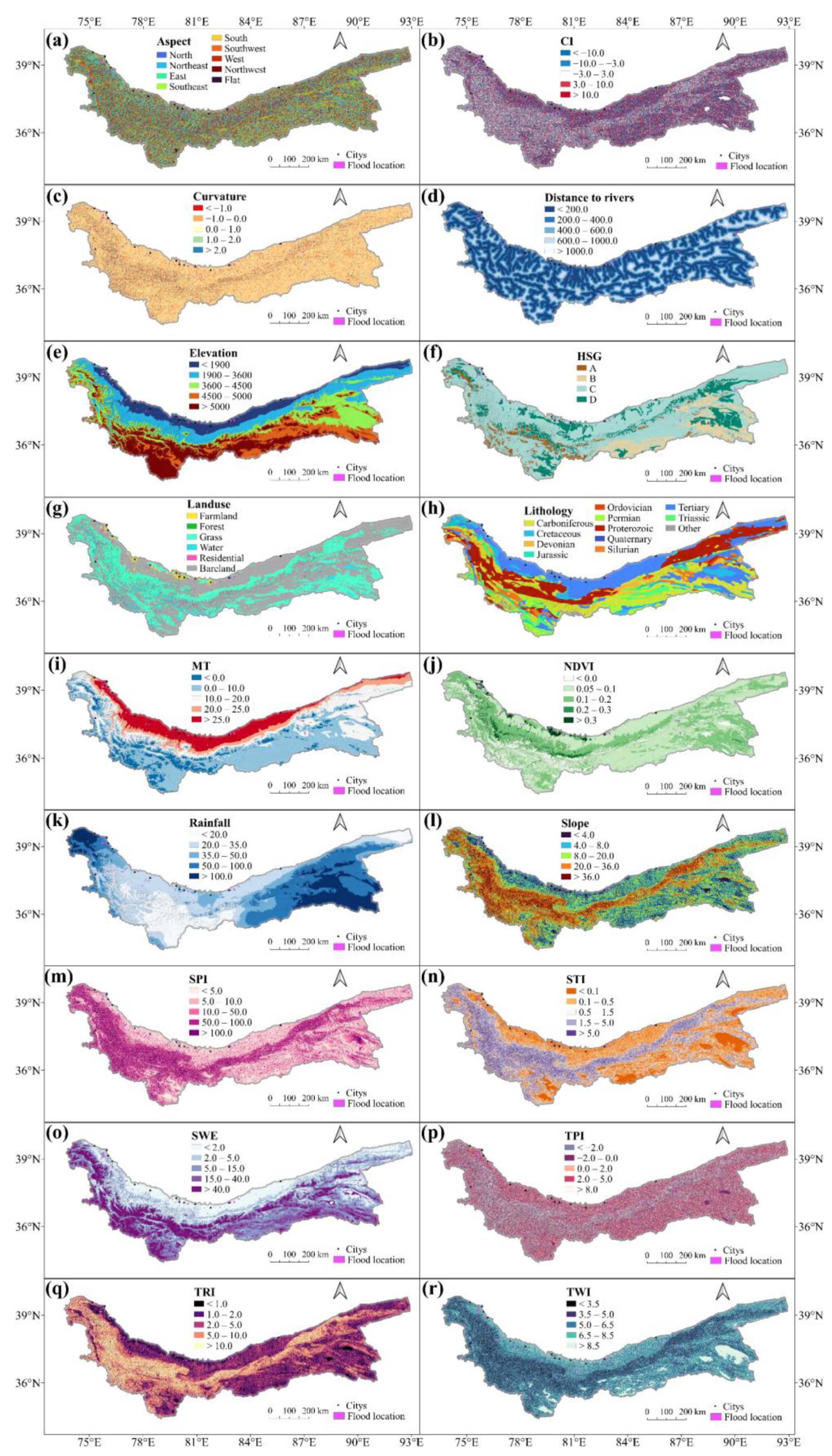
Using the sensitive flood conditioning factors is critical in generating an accurate flood-susceptibility map [53]. To select the most influential factors, 18 factors affecting snowmelt floods were considered based on historical studies [8,55,56,57,58,59,60], which cover topography, meteorology, human activities and snow. It is worth noting that the formation of snowmelt-type floods is related to snow and thermal conditions, in addition to the influence of topography and rainfall [9]. Snowmelt and high temperatures should be additionally considered when studying snowmelt-type floods to distinguish them from other types [61,62]. In terms of subtypes, warming floods are mainly caused by high temperatures, while mixed floods are influenced by a combination of high temperatures and rainfall [63]. Table 1 contains a summary of these conditioning factors. The spatial distribution map of the data is categorized according to the natural breakpoint approach (Figure 2).
The spatial resolution of all the conditioning factors was resampled to 30 m to maintain uniformity on a spatial scale. Long-term multitemporal data related to meteorological factors were processed by taking multi-year averages. A small portion of the few data that could not cover the historical flood duration started from the earliest available time. In addition, the data-standardization method was used to solve the problem of an inconsistent range of data values [64], which can prevent model parameters from failing to converge during model training. The data were input as the same size two-dimensional arrays. Flood events with different ranged sizes were divided by a fixed matrix to achieve incremental data, yielding 1105 positive sample datasets. An equal number of matrices was randomly generated as negative sample datasets in other areas which do not have snowmelt flooding as in the study area to meet the model’s training needs. Referring to the division basis of DL-related studies [48], while ensuring that the model is adequately trained, the whole dataset is divided into training and validation sets in the ratio of 7:3.

2.3.1. Terrain Factors

Terrain factors are represented by Digital Elevation Models (DEM) and derived maps. The DEM data source was from Global Digital Elevation Model Version 3. The derived data were obtained by extracting and calculating the DEM with a spatial resolution of 30 m. There are elevation, slope, aspect, convergence index (CI), curvature, distance to rivers, topographic position index (TPI), topographic ruggedness index (TRI), stream power index (SPI), sediment transport index (STI) and terrain wetness index (TWI). Elevation is one of the most critical factors affecting floods, and flooding is inversely proportional to elevation. The higher the altitude, the lower the chance of flooding and vice versa happening [65]. Slope is an essential surface characteristic that affects floods by affecting surface runoff velocity and vertical seepage [66]. Aspect is defined as the direction of the most prominent slope on the terrain surface. As different slope directions respond differently to precipitation, they affect the direction of flood flow while maintaining soil moisture [67], which makes aspect influences flooding indirectly [26]. Curvature is a factor of runoff, which describes the degree of slope deformation and is used in modeling flood susceptibility since curvature affects the water budget of floods [68,69]. CI is a morphological characterization factor that quantifies the convergence of the river network [70], with negative values highlighting valleys and positive values highlighting the characteristics of the inter-alluvial surface. Most affected flooded areas are usually near rivers [71]. Distance to rivers is an essential moderating factor in determining which areas are affected [72]. Thus, distance to rivers directly affects flooding. TPI is often used to distinguish topographic slope positions, with positive values indicating a central store above the surrounding mean and negative values indicating a lower one below the mean [73]. TRI is one of the main influencing factors of flood events. It depends on the local topography of the study area. Higher flood probabilities are associated with lower TRI values [57]. SPI refers to the ability of a river to transport sediment and erode its bed during floods, which has an essential impact on the river system [74]. STI is directly related to changes in the elevation and structure of the riverbed, which can increase the frequency of floods and thus leading to damage to the foundation [75]. For the occurrence of floods, TWI is an influential factor by which the differences in wetness in the study area are spatially represented by this index [76].

2.3.2. Meteorological and Snow Factors

Rainfall was chosen as one of the main influencing factors for snowmelt flooding. The reason is that high-intensity rainfall over a short period can cause snowmelt and superimpose itself to trigger snowmelt flooding [77,78,79]. Similarly, higher temperatures can also trigger snow melt, thus leading to the formation of snowmelt floods [78], and the maximum temperature (MT) can reflect the potential risk of snowmelt floods and is a valid response indicator for snowmelt flood assessment [80,81]. The snow water equivalent (SWE) is of great significance for allowances and water use, as it describes the amount of water stored in the snowpack [82]. It better expresses the contribution to runoff and thus indirectly affecting snowmelt flooding compared with snowpack depth [82,83]. Therefore, it is used to assess the susceptibility to snowmelt flooding. The rainfall and MT maps represent annual averages from 1999 to 2020. These data were obtained from the Loess Plateau Subcenter of the National Earth System Science Data Center of the Ministry of Science and Technology of China (loess.geodata.cn, accessed on 17 January 2022) at a raw spatial resolution of 1 km. SWE maps represent mean values from 2002 to 2020, and data were obtained from the AMSR-E/Aqua L3 Global Snow Water Equivalent EASE-Grids. The raw spatial resolution is 10 km, and this paper used a proven method of combining the raw SWE dataset with the MODIS/Aqua Snow Cover 8-Day L3 Global 500 m SIN Grid, Version 6 to increase the spatial resolution of the data to 500 m [60,84,85].

2.3.3. Other Factors

Other factors include normalized difference vegetation index (NDVI), hydrological soil group (HSG), lithology and land use. NDVI is an indicator that expresses vegetation’s denseness, and it strongly influences flooding [86]. It is widely accepted that areas with low vegetation density are prone to flooding [87]. NDVI maps represent the mean values from 2002 to 2020, with data from MODIS remote sensing data products and a raw spatial resolution of 250 m. HSG is a soil classification based on minimum permeability, with different runoff potentials for each group [88]. It affects the rate of water infiltration and, finally, the storage potential of the surface, which in turn affects flooding [89]. HSG components are divided into four groups: A, B, C and D. The soil in group A has the minimum runoff potential, and the soil in group D has the maximum runoff potential. The raw data were obtained from soil data provided by the National Cryosphere Desert Data Center (ncdc.ac.cn, accessed on 23 January 2022) with a spatial resolution of 10 km. Lithology determines the structure of drainage patterns, and different lithologies have different soil porosity and infiltration rates [90], which significantly impact the development of floodplains [38]. Therefore, lithology is necessary for the spatial prediction of floods. The original data is a geological map of the Xinjiang Uygur Autonomous Region at a scale of 1:5,000,000, and the available data were obtained by rasterization. The lithological grouping of the study area includes Quaternary, Tertiary, Cretaceous, Jurassic, Triassic, Permian, Carboniferous, Devonian, Silurian, Ordovician, Proterozoic and others. Land use categories directly control the generation and infiltration of surface runoff [91], and different types of land use influence flood frequency by affecting runoff, which helps to identify flood-prone areas [91,92]. The raw data were obtained from the China Resources and Environment Science and Data Center with a spatial resolution of 1 km. The classification includes farmland, forest land, grassland, waterbody, residential land and bare land.

2.4. Methodology

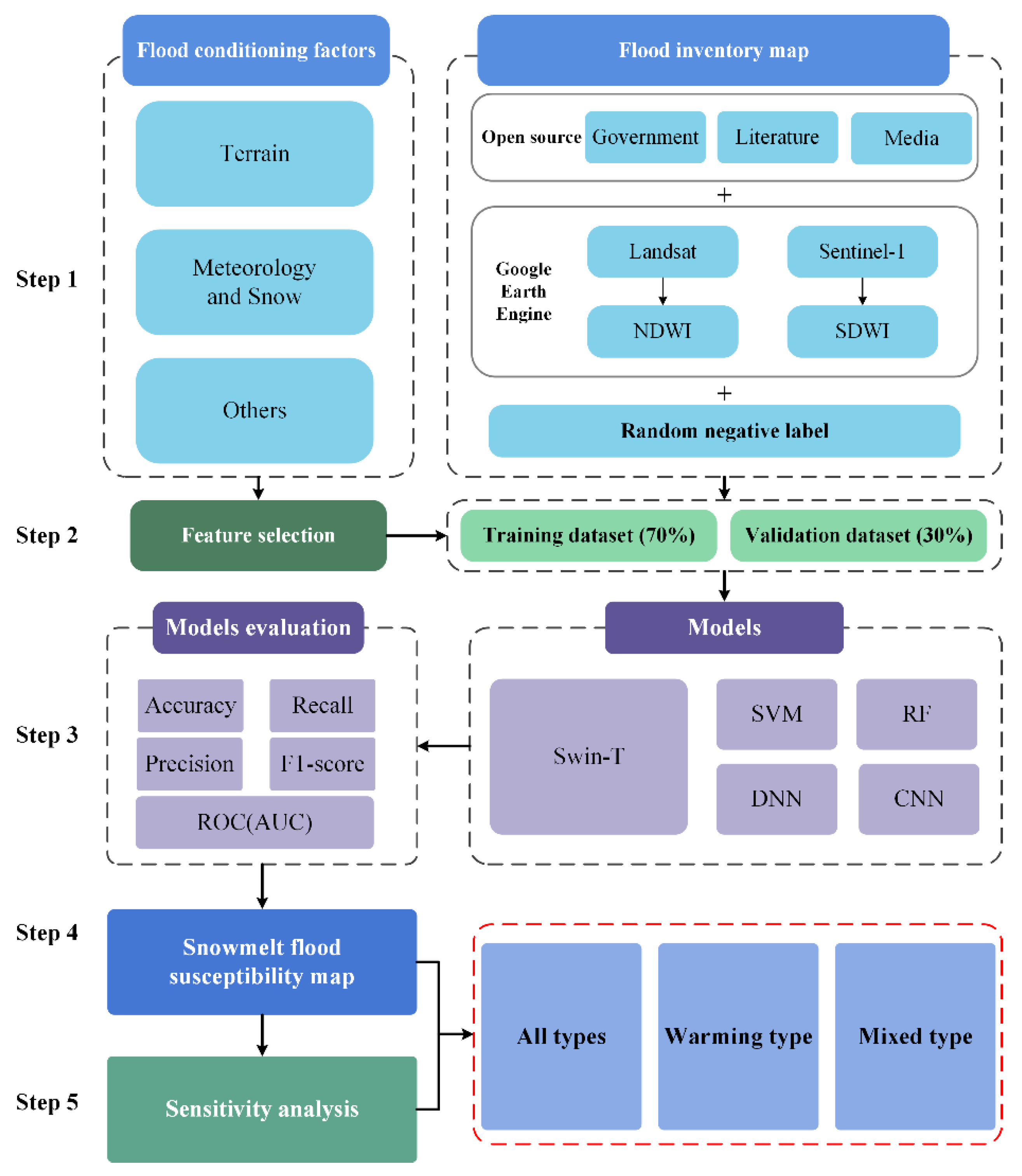
In this research, five models were used to evaluate the susceptibility of snowmelt floods in the Kunlun Mountains. The Swin Transformer (Swin-T) is the most novel one of these methods, in addition to two traditional ML models, support vector machine (SVM) and random forest (RF), and two DL models, deep neural network (DNN) and convolutional neural network (CNN). The flow chart of the method used in this study is shown in Figure 3, consisting of five parts: (1) Prepared the historical flood inventory and selected the appropriate flood conditioning factors. (2) Constructed training and validation datasets by screening the flood-influencing factors based on ReliefF and multicollinearity analysis methods. (3) Constructed and trained several models, including Swin-T, and then evaluated their performance for comparison. (4) Based on the best-performing model, different snowmelt flood susceptibility maps were generated using data inventory data screening. (5) Sensitivity analysis of different snowmelt floods was performed for the conditioning factors.

2.4.1. Feature Selection

Filtering the input features to remove those with poor classification ability can effectively avoid the training difficulties associated with high data dimensionality [28] and improve the stability of the model [93]. The influencing factors should be independent; therefore, it is necessary to test the predictors for multicollinearity [36]. The variance inflation factor (VIF) has been widely used in detecting flood susceptibility factors and has the characteristics of accuracy and efficiency [48,94]. Therefore, this study used VIF to quantify the potential influence of 18 snowmelt flooding moderators on the model. VIF > 9 and very low correlation coefficients indicate the presence of multicollinearity among the factors [95], and it is strongly recommended to exclude moderators with VIF > 9 from modeling. In addition, ReliefF is one of the most well-known methods for selecting influential variables [96], which effectively estimates the quality of attributes in the problem of variable dependence [97]. Therefore, the ReliefF method was used to assess various factors’ effective contribution to the classification. The method uses random feature sampling to estimate the quality of attributes based on the degree of differentiation (distance) of attribute values between close instances [96]. The equation based on the feature weight update calculation is as follows:
W ( A ) = W ( A ) j = 1 k d i f f ( A , R i , H j ) m k + C c l a s s ( P ) [ P ( C ) 1 P ( c l a s s ( R i ) ) × j = 1 k d i f f ( A , R i , M j ( C ) ) ] × ( m · k ) 1
where W ( A ) represents the updated feature weight, Function d i f f ( A , R i , H j ) indicates that sample one and sample two differ in feature A. The contribution for each class of misses is weighted by the prior probability of that class P ( C ) (estimated from the training set). P ( c l a s s ( R i ) ) represents the sum of the probabilities for the miss classes.

2.4.2. Models

(1)
Swin Transformer (Swin-T)
Swin Transformer (Swin-T) is a relatively new deep learning model that abandons the convolutional stack structure of CNNs and uses an encoder approach to preserve the global features of the data [40]. This model relies on hierarchical transformer blocks and window-shifting transformer structures to reduce computational complexity by not overlapping windows, overcoming the lack of global effects and avoiding the loss of connectivity between each window [98]. Like the convolution process of CNN, the data are split among the models, but the spatial connections between them are retained in Swin-T. Figure 4 shows the Swin-T structure used in this study.
The framework of the whole model consists of a Patch Partition module and multiple stages containing Swin-T blocks. The input data to the model is a multi-layer image consisting of flood conditioning factors. The Patch Partition module is responsible for segmenting and encoding the input data, and then merging the adjacent small blocks into a structure with deeper layers [40]. The linear embedding module in stage 1 is used to change the number of input layers to meet the input of the Swin-T block. In contrast, the Patch Merging layer included in the rest stages is like the pooling operation that reduces the computational complexity without losing information. The final output of the model is the probability of whether it is a flood or not.
The Swin-T block is the most important module in this structure, and it comprises two shifted window-based multi-head self-attention (W-MSA and SW-MSA) modules, a 2-layer Multilayer Perceptron (MLP) with Gaussian Error Linear Unit (GELU) nonlinearity in the middle. Before each MSA module and each MLP, a LayerNorm (LN) layer is applied, and a residual connection follows each subblock [40]. The whole block can be expressed as follows:
z ^ l = W MSA ( LN ( z l 1 ) ) + z l 1
z l = MLP ( LN ( z ^ l ) ) + z ^ l
z ^ l + 1 = SW MSA ( LN ( z l ) ) + z l
z l + 1 = MLP ( LN ( z ^ l + 1 ) ) + z ^ l + 1
where z ^ l and z l represent the outputs of the (S)W-MSA and the MLP of l t h block. The shift operation of the window in the MSA block is the key to the model’s ability to address the global information deficit (Figure 5). The movement of the window changes the scope of information perception and creates connections between otherwise unconnected data, allowing global information to be preserved [99]. Additionally, the multi-head self-attention mechanism can be expressed as follows:
M u l t i H e a d ( Q , K , V ) = C o n c a t ( h e a d 1 , , h e a d h )
h e a d 1 = A t t e n t i o n ( Q W i Q , K W i K , V W i V )
A t t e n t i o n ( Q , K , V ) = S o f t M a x ( Q K T d + B ) V
where Q , K , V R M 2 × d , Q stands for query, which will be matched with each K in the follow-up, K stands for key, which will be matched by each Q in the follow-up, and V stands for the extracted information, and d represent the dimension of query or key.
(2)
Support vector machine (SVM)
SVM is a classical and general machine learning method [100] widely used in flood susceptibility assessment [90]. SVM adopts the kernel function approach to map the original data to multiple dimensional feature space and constructs a hyperplane to achieve classification. The model’s performance depends on whether the choice of kernel function matches the target. The current main kernel functions include linear kernel, sigmoid kernel, radial basis, and polynomial kernel. The radial basis sum function was used in the study because it outperformed other kernel functions in assessing flood susceptibility [39].
(3)
Random Forest (RF)
The RF model is a representative machine learning model with an efficient combination of multiple decision trees (DTs). Each DT is constructed with bootstrap samples of the data, and the majority result of all DTs determines the model’s outcome [101]. Therefore, RF can avoid the problems of noise and overfitting and effectively perform the tasks of regression and classification. As one of the excellent representatives of integrated learning, this model has more advantages in flood-susceptibility mapping [102,103].
(4)
Deep neural network (DNN)
DNN is an artificial neural network with multiple hidden layers, enabling complex data transformation by increasing the number of hidden layers, making it better applicable to variable relations with complex relationships [30]. From the technical point of view, the model has no rule of thumb, and its decision process is influenced by the problem’s complexity and the data set. DNN is a feed-forward neural network that uses backpropagation for training and reduces the training difficulty of the network through different activation functions and optimization functions. As one of the popular deep learning algorithms, it has been used several times in flood susceptibility assessment [30,31]. This study used a DNN model consisting of an input layer, three hidden layers and an output layer to model the susceptibility to snowmelt flooding.
(5)
Convolutional neural network (CNN)
CNN is a multilayer feed-forward neural network that automatically extracts valuable features from original data, and it has shown powerful performance in several flood hazard applications [104,105]. The architecture improves the structure of the hidden layer based on DNN by changing it from a fully connected layer to a combination of different numbers of convolutional and pooling layers. The convolutional layer uses convolutional kernels to extract complex features, which usually follow the pooling layer responsible for down sampling and reducing the computational cost. The present study constructed a visual geometry group (VGG) model, a classical convolutional neural network model with excellent performance [106]. The model consists of thirteen convolutional layers, three fully connected layers, five pooling layers and a SoftMax layer for final classification.
All models in this study were built on a dell computer from Xinjiang, China, configured with an i9-11900k processor, 128 G RAM and RTX A4000 graphics card. All model implementations are based on the python language and related libraries from the Python Software Foundation in Delaware, USA, where the Python version is 3.9. Hyperparameter optimization is implemented through the Optuna framework [107], which contains many excellent hyperparameter sampling algorithms for optimizing ML and DL models. The hyperparameters are shown in Table 2. To avoid model overfitting and to ensure model robustness, the training results of all models are based on the lowest loss convergence achieved in the validation set.

2.4.3. Model Evaluation

The model was evaluated using four widely used indices, including accuracy (A), precision (P), recall (R) and F1-score (F). The calculation of these indices relies on the confusion matrix values. The model’s positive and negative samples correctly predicted are true-positive (TP) and true-negative (TN). In contrast, the positive and negative samples that are incorrectly classified are called false-positive (FP) and false-negative (FN). The above four indices are calculated as follows:
A = T P + T N T P + F P + T N + F N
P = T P T P + F P
R = T P T P + F N
F = 2 P R P + R
In addition, the study uses receiver operating characteristic (ROC) and area under curve (AUC) to respond more visually to the good or bad performance of the model [108], and they are widely used to assess the accuracy of sensitivity maps [39,109]. The ROC curve was constructed with “1-specificity” as the X-axis and “sensitivity” as the Y-axis. “1-specificity” is the false positive rate (FPR), “Sensitivity” represents the true positive rate (TPR), and they are calculated as follows:
F P R = F P T N + F P
T P R = T P T P + F N
AUC = 0 is considered no informative result, AUC = 0.5 is considered no classification performance, and AUC = 1 means that the simulated results have an excellent spatial agreement with the actual labels.

2.4.4. Sensitivity Analysis

Sensitivity analysis is a general method for quantifying the contribution of variables or parameters to the variability and uncertainty of different kinds of numerical model outputs [110]. The Jackknife test is often used for statistics of model characteristics [26], most AUC-based statistical coefficients rely on it [111], and it is considered to have high power for a wide range of practical problems [112]. Therefore, the Jackknife test was used to assess the factor’s sensitivity to flooding in the study. This test compares predictions based on all dependent variables with predictions that deliberately exclude one dependent variable, observing the reduction in AUC relative to the original value [113]. The percentage of relative decrease (PRD) is the indicator evaluated by this test method. The effect of the excluded factor is considered more pronounced if the PRD is reduced by more. The PRD is calculated as:
P R D i = 100 × | A U C o A U C i | A U C o
where A U C o is the original AUC value including all factors, and A U C i is AUC value when the i t h factor has been removed.

3. Results

3.1. Feature Selection

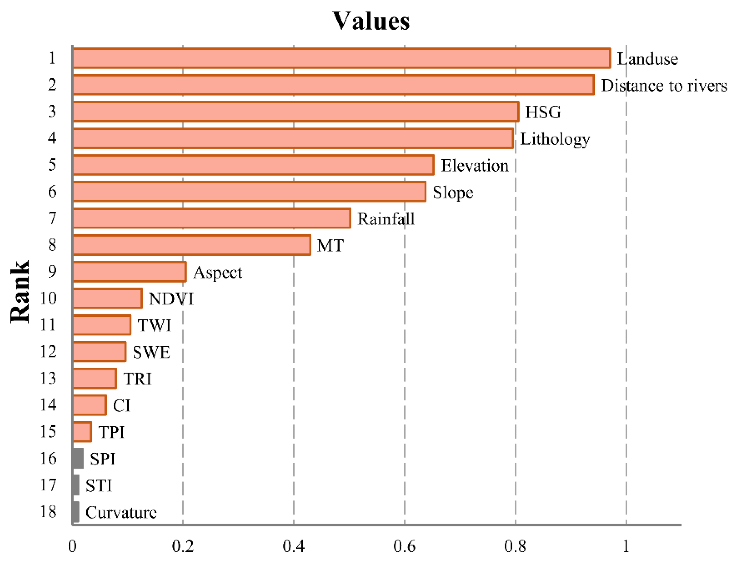
The outcomes of the multicollinearity diagnostic test (Table 3) showed that the VIF was greatest for elevation (value = 7.2), followed by curvature, slope, TPI, TRI, SPI, STI, MT, NDVI, SWE, lithology, land-use, TWI, distance to rivers, CI, HSG and rainfall. The results also indicated that there was no collinearity problem among 18 potential factors for involving flood susceptible models. In addition, the study calculated separately for the warming, mixed and all types of flood data to avoid the errors associated with the random sampling of the ReliefF method, then the average of these results was used as a reference for classification ability (Figure 6). Result suggested that land use, distance to rivers, HSG, lithology, elevation and slope had a strong classification power (values > 0.6) in the flood model of the study area. As factors specific to snowmelt flooding, MT and SWE were in the middle of the result ranking, and their classification performance should not be neglected. In contrast, the lower-ranked factors were related to terrain: SPI, STI and curvature were at the end of the ranking. It is noteworthy that these three factors ranked in the last three places in all random feature sampling results, although there were differences in the order. Therefore, to ensure the prediction model’s accuracy, these three factors were eventually removed from the input features while retaining the other fifteen conditioning factors as input factors for the model.

3.2. Model Comparison and Validation

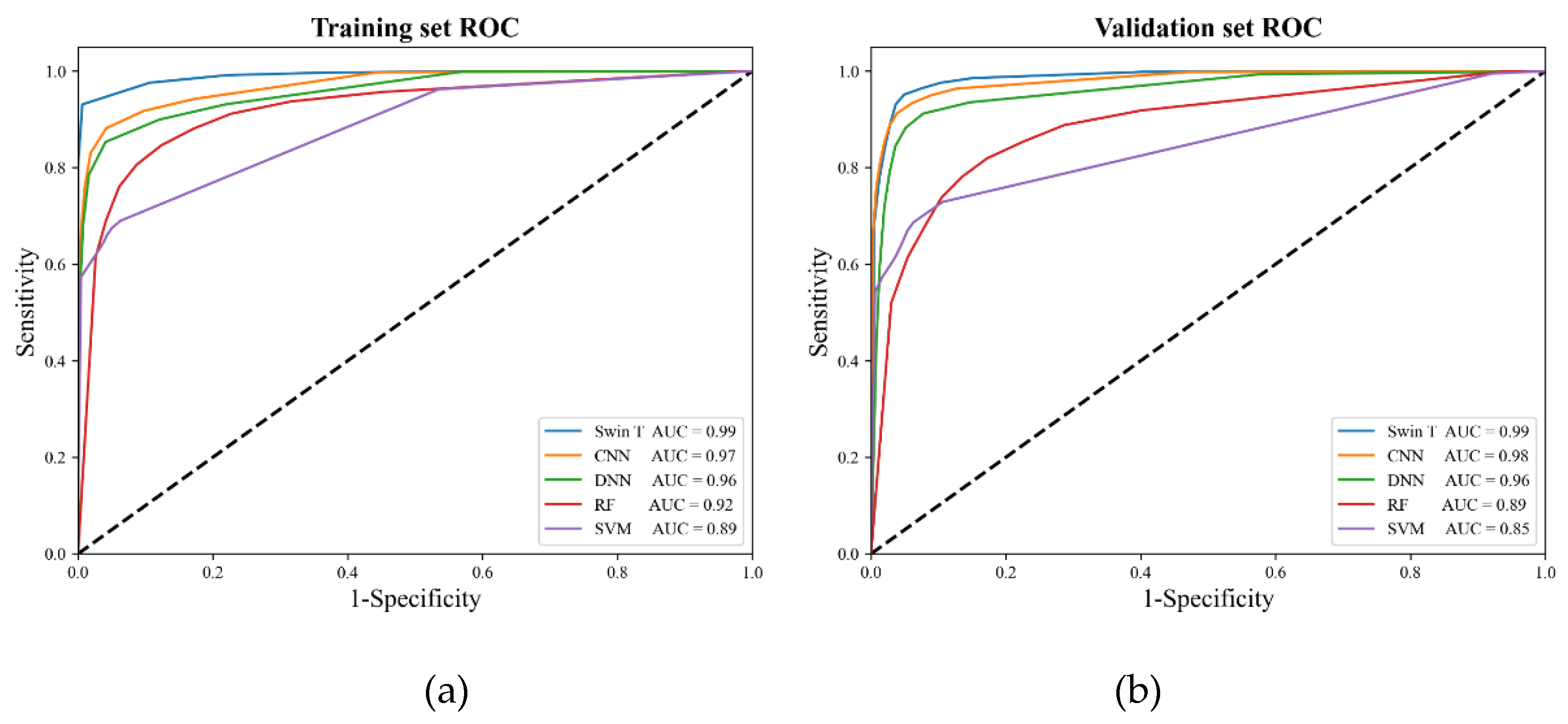
Five susceptibility models (Swin-T, SVM, RF, DNN, CNN) were evaluated on the training and validation sets using various standard quantitative metrics (Table 4 and Figure 7). The results showed that the models had the same ranking by data accuracy on both the training and validation sets, with the highest accuracy being Swin-T (99.55% and 96.07%), followed by CNN, DNN, RF and SVM. The highest precision (99.27% and 96.55%) was obtained for the random forest model on both the training and validation sets. On the other hand, CNN had the highest Recall (97.48%) on the validation set. Other than that, Swin-T won in all the remaining metrics, including having the highest Recall (100%) on the training set and having the highest F1-score (99.55% and 96.05%) on both the training and test sets. The results showed that the Swin-T model has the highest accuracy and high confidence on all datasets, which could provide accurate snowmelt flood susceptibility maps.
The ROC results showed that the Swin-T model achieved the highest AUC value (0.99) on both the training and test sets. The remaining models were CNN (AUC = 0.97 and 0.98), DNN (AUC = 0.96 and 0.96), RF (AUC = 0.92 and 0.89), and SVM (AUC = 0.89 and 0.85) in order. All models used in this study attained satisfactory flood sensitivity assessments (AUC > 0.85). The analysis of ROC showed that Swin-T had the relatively best predictive power, as well as the most robust generalization ability, and the other models were ranked closely to the performance evaluation results in previous studies [31,39]. Therefore, Swin-T was finally selected to generate snowmelt flood-susceptibility maps.

3.3. Flood Susceptibility Mapping

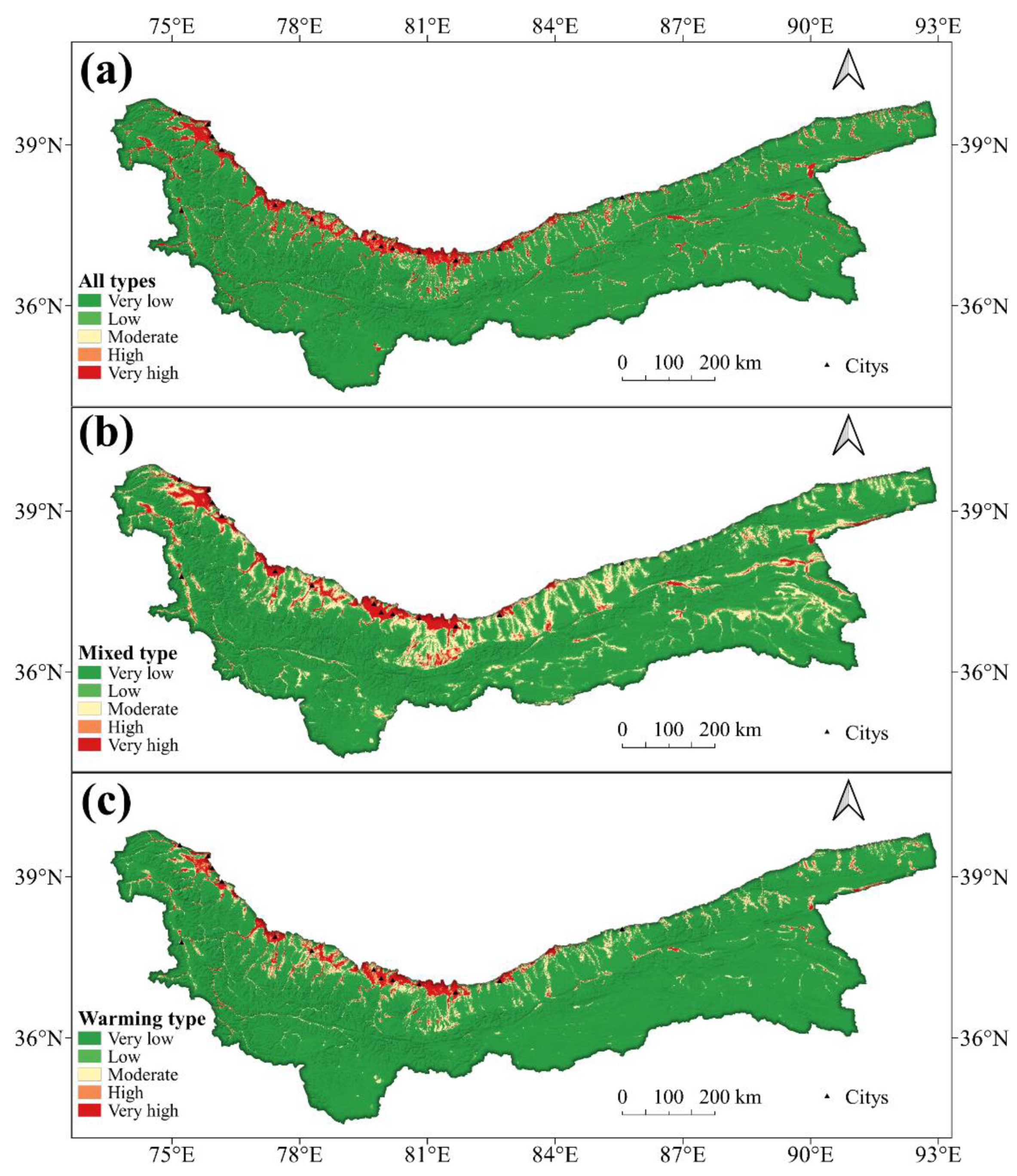
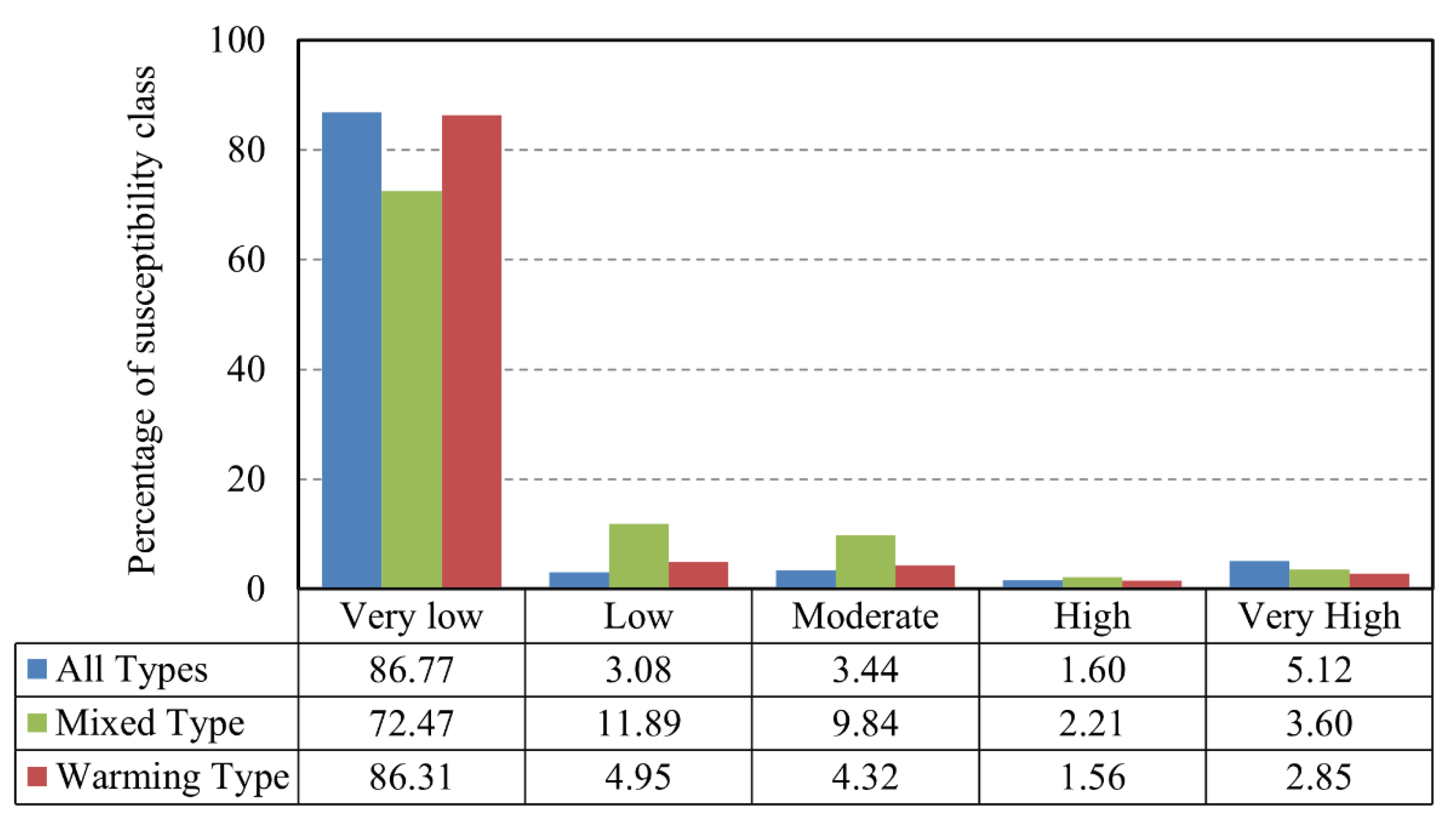
The research mapped snowmelt flood susceptibility separately using data for different flood types, including warming, mixed, and all types containing. These maps were classified into five classes: very low susceptibility, low susceptibility, moderate susceptibility, high susceptibility and very high susceptibility using the natural break classification method (Figure 8). In addition, the study compared the susceptibility classification of diverse types by counting the specific proportions of the different susceptibility classes (Figure 9).
For all types of snowmelt floods, the areas with high and above susceptibility are primarily along rivers, concentrated in the low-elevation areas in the north-central and north-west of the study area, with a high overlap with the distribution of cities. At the same time, only a tiny part of the eastern regions fell into both classes. From the perspective of area proportion, the proportion of high and above classes was only 6.72% of the entire study area, and the susceptibility of most areas is low. These areas have the characteristics of high altitude and are far from the river. Compared with all types of assessment results, in the mixed-type susceptibility assessment results, although the distribution of high and above classes was also concentrated in the urban area at the border of the study area, the distribution of low susceptibility areas in this result was significantly reduced. In terms of area, there was a 14.3% decrease in the low-susceptibility areas, and this part was more often reclassified as low- and moderate-susceptibility areas. In contrast, the area proportion of high susceptibility and above classes did not change much for about 5.81%, and the sporadic distribution was significantly reduced. In the evaluation results of warming-type snowmelt floods, the sporadic distribution of high and above classes was the least among the three results, and the concentrated distribution was more evident in the urban areas of the central and northwestern regions. However, the proportion of its area was further decreased simultaneously. Correspondingly, the proportion of low- susceptibility and very low classes increased further, reaching 91.26%, and there were almost no high- susceptibility areas in high-altitude areas. The abovementioned outcomes showed significant differences in the susceptibility zoning of warming and mixed snowmelt floods.
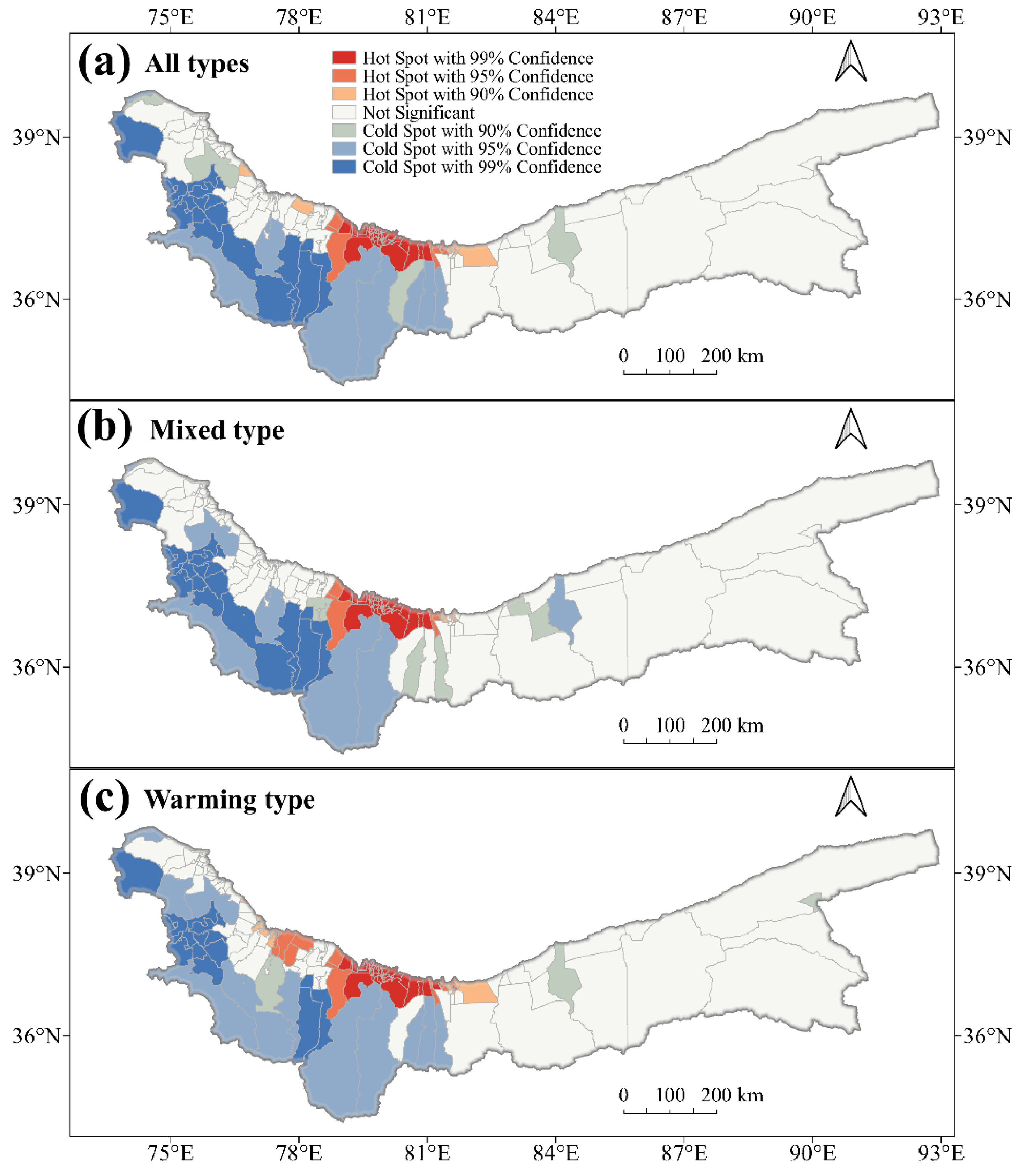
A hotspot analysis tool was used to explore further spatial characteristics of the snowmelt flood susceptibility maps of 227 townships in the study area (Figure 10). The results showed that the different types of snowmelt floods had highly similar pattern characteristics, i.e., the hotspot areas with high-value aggregation which were mainly distributed in the north-central part and showed a concentrated contiguous pattern. The warming type had the most 105 high-value hotspot areas in comparison, and the rest were all types (70) and mixed types (64). Moreover, the distribution of hotspot areas with low-value aggregation extended from the southwestern part of the study area to the western region, again showing a contiguous distribution. Besides, most of the eastern part of the study area was not significant. The high susceptibility to snowmelt flooding in the study area showed a small spatial concentration in the north-central part. Therefore, this region is highly susceptible to snowmelt flooding, and the regional decision makers should pay attention to snowmelt flood prevention.
For further confirmation of the reliability of the results, we conducted a regional statistical analysis on the distribution of snowmelt flood events in different prone areas (Table 5. The proportion of these flood events in different susceptibility classes reflect the reasonableness of the results of the susceptibility assessment [36]. Among the three susceptibility evaluation results, more than 90% of the historical snow-melt flood events were in the high and above classes, which indicates that the evaluation results of snowmelt flood susceptibility based on the Swin-T model had high reliability.

3.4. Sensitivity Analysis

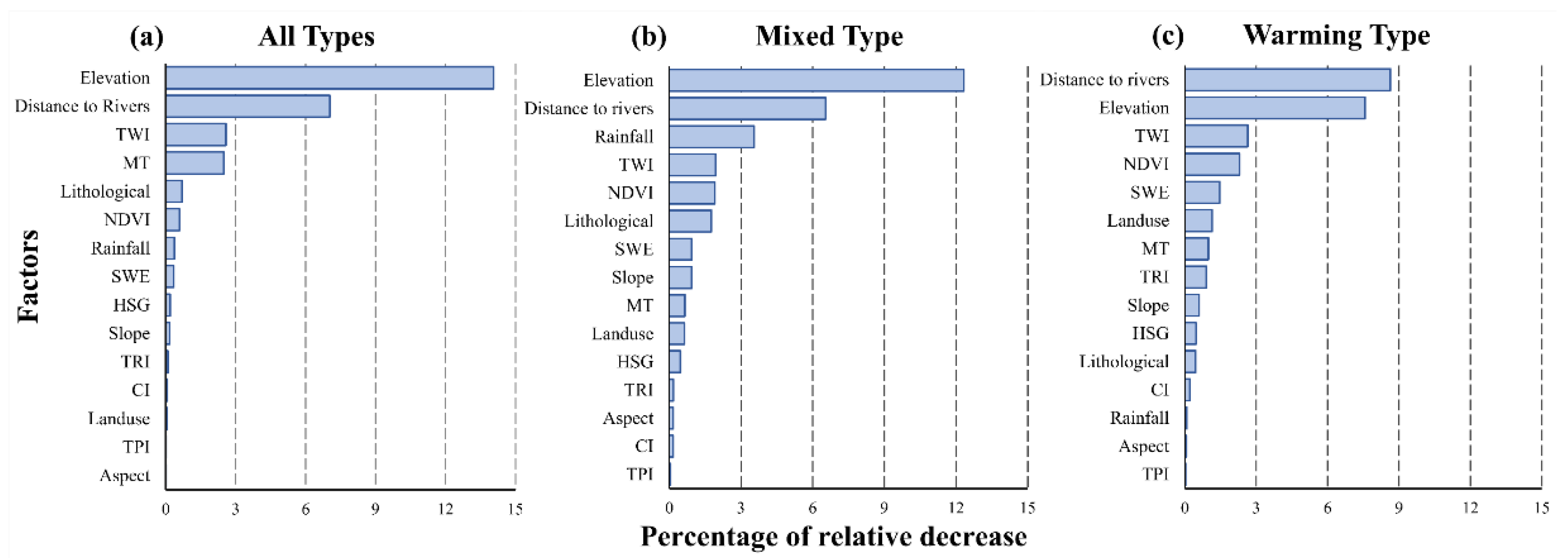
The sensitivity tests for the fifteen snowmelt flood factors were performed using the Jackknife test method, and the results were ranked from highest to lowest in terms of PRD values (Figure 11). In this study, for all ranking results, elevation and distance to rivers are more influential on snowmelt flooding and have higher sensitivity (PRD > 6) than other factors. Elevation had a more major influence than the distance to rivers among all types and mixed types. In contrast, in the warming type, the PRD of these two factors was close, with distance to rivers being the more sensitive factor (PRD = 8.6) but less different from elevation (PRD = 7.6). In all ranking results, all factors at the bottom (PRD < 0.1) were topography-related, including TPI, CI and aspect. The small effect of rainfall in warming floods (PRD < 0.1) suggested that the main contribution of runoff in this type comes from snowmelt, which is consistent with the view that warming snowmelt floods are almost unaffected by rainfall [21]. In contrast, the rainfall effect had a higher sensitivity in mixed snowmelt floods (PRD = 3.5), indicating a higher percentage of rainfall in the runoff than the snowmelt factor (PRD = 0.9). The two types were effectively distinguished. It is worth mentioning that MT and SWE, as factors unique to snowmelt flooding, were in the middle-ranking (PRD > 0.5) of all the test results, which implied that they have some contribution to snowmelt flood susceptibility. Therefore, it can be concluded that the model successfully identifies the relationship between the influencing factors and snowmelt flooding.

4. Discussion

A critical prerequisite for flood hazard prevention and reduction is the adoption of appropriate flood modeling [18,114], so it is necessary to explore the possibility of applying new techniques in snowmelt flood susceptibility assessment. Taking Kunlun Mountain as an example, we tried to apply an advanced model Swin Transformer to assess snowmelt flood susceptibility which so far has not been used in the field of flood-susceptibility assessment and compare it with the methods used before such as SVM, RF, DNN and CNN. Among the methods, SVM and RF are widely applied for landslide susceptibility modeling [115,116], flood-susceptibility modeling [31,117] and gully-erosion modeling [118,119,120]. DNNs and CNNs have also become popular as recent methods in natural hazard risk assessment [45,121]. As more and more studies no longer consider floods as a point phenomenon [122], the explanatory factors of the surrounding environment are gradually under consideration in flood risk studies. More efficient use of spatial information may mean better performance results for data and studies that emphasize spatial information [122]. The use of two-dimensional (2D) data as input preserves the spatial information well, and the efficient use of spatial information enables DL methods to automatically learn more valuable features within the model [31]. 2D data are split into individual pixels in traditional ML methods, which cut off the connections between points, leading to the destruction of the spatiality of the data [123]. In contrast, CNN models input 2D data as a whole and obtain more accurate results than single-point input (AUC = 0.98). The model effectively uses the spatial information of the data. However, as mentioned in the introduction, CNNs can only retain local spatial information and internal operations to dissolve the global features. Swin-T, which encodes globally, has the best performance (AUC = 0.99), indicating that preserving the spatial integrity of the data allows the model to learn more internal features that are beneficial for evaluation. In the research, retention of the data spatial information integrity proved helpful for improvement of model performance. Admittedly, there are still some challenges the Swin-T model will face. Considering the trade-off between the complexity of the model structure and the training problem, using Swin-T with a deep structure requires tunes a large number of parameters, which makes it risky when migrating applications, it’s a limitation of DL methods in the field of flood assessment as well. Besides, in future research, more common ML models such as MAXENT and ANN should be included in the comparison instead, making the model performance amount results more convincing. Therefore, to avoid the possibility of specialization, the Swin-T model needs more application cases to demonstrate its generalization ability for performance improvement in flood-susceptibility studies.
In addition to the choice of the model itself, the composition of flood-regulating factors significantly impacts the assessment of flood susceptibility. Unlike terrain factors, meteorological factors are subject to more rapid change. The spatial and temporal variations of vital sensitive factors such as temperature, snowpack and rainfall are closely linked to future snowmelt flooding in the study area. The present outcome also proved that these moderating factors are non-negligible in snowmelt flood susceptibility. However, an appropriate number of conditioning factors should be selected when assessing flood susceptibility. Too many input features may negatively affect the model to make an accurate assessment [28]. Some DEM-derived data (e.g., TPI, CI, STI) appear to have limited impacts on snowmelt flooding compared with other factors in this study. Therefore, when there are few model parameters, researchers should focus on influences related to meteorological factors and human activities to improve data quality and save time and cost. It is worth noting that the contribution of aspect and slope to snowmelt flooding seems to be limited in the study area, which makes them less critical. However, in some flood-susceptibility studies, aspect or slope were greatly affected [26,36,124]; the difference may be a result of the specific topography of the Kunlun Mountains region, which should be analyzed in depth in future. In addition, flood frequency should be an important influencing factor for flood susceptibility [125], but this factor seems to receive insufficient attention in flood-related ML methods. In the case of snowmelt flooding, the permafrost extent or ratio is also an essential influencing factor [126]. For the reasons out of prudence and controlling the number of features, some other additional snowmelt flooding influencing factors were not added; so, in future studies, attempts to consider these influences may achieve better assessment accuracy.

5. Conclusions

Flood-susceptibility maps are generated by collecting and analyzing data from various sources combined with modeling approaches to improve understanding of the spatial distribution probability of snowmelt floods. In this study, Swin-T was used to model and evaluate the sensitivity of snowmelt floods in the Kunlun Mountains region of Xinjiang. The performance was compared with machine learning and deep learning methods such as SVM, RF, DNN and CNN. Susceptibility maps for different types of snowmelt floods were generated with the combination of historical snowmelt flood data and condition factors in the study area. Then, sensitivity analysis was performed for different types of conditions. In general, the main conclusions of this paper are summarized as follows.
(1)
The Swin-T-based approach had the most accurate and robust results. It successfully determined the relationship between the conditioning factors and the occurrence of snowmelt flooding.
(2)
Elevation and distance to rivers influenced snowmelt flooding in the study area. Rainfall and snow water equivalent were the dominant natural factors for mixed and warming types.
(3)
The north-central area of the Kunlun Mountains is highly susceptible to snowmelt floods.
The results of this study can provide a useful reference for regional decision-makers in planning and policy development for snowmelt flood management and prevention.

Author Contributions

Conceptualization, R.Y., G.Z. and A.B.; methodology, R.Y. and P.H.; software, R.Y. and P.H.; validation, Y.L.; formal analysis, R.Y.; investigation, R.Y.; resources, R.Y. and Y.L.; data curation, R.Y.; writing—original draft preparation, R.Y.; writing—review and editing, G.Z., W.X. and A.B.; supervision, A.B.; funding acquisition, Y.L., W.X. and A.B. All authors have read and agreed to the published version of the manuscript.

Funding

This research was funded by the Open Project of Key Laboratory of Xinjiang Uygur Autonomous Region, grant number 2018D04027, the 2020 Qinghai Kunlun talents—Leading scientists project, grant number 2020LCJ02 and the Key Research and Development Program of Xinjiang Uygur Autonomous Region, grant number 2022B03001-3.

Acknowledgments

Acknowledgement for the data support from Loess Plateau SubCenter, National Earth System Science Data Center, National Science & Technology Infrastructure of China.

Conflicts of Interest

The authors declare no conflict of interest.

References

  1. Pascaline, W.; Debarati, G.-S.; Denis, M.; CRED; UNISDR. The Human Cost of Weather-related Disasters 1995–2015; CRED: Bengaluru, India; UNISDR: Geneva, Switzerland, 2015; p. 30. [Google Scholar]
  2. Ahmadisharaf, E.; Tajrishy, M.; Alamdari, N. Integrating flood hazard into site selection of detention basins using spatial multi-criteria decision-making. J. Environ. Plan. Manag. 2016, 59, 1397–1417. [Google Scholar] [CrossRef]
  3. Wang, H. Study on Three-Dimensional Visualization of Snowmelt Flood. Master’s Thesis, Shihezi University, Shihezi, China, 2016. [Google Scholar]
  4. Hock, R.; Rees, G.; Williams, M.W.; Ramirez, E. Preface—Contribution from glaciers and snow cover to runoff from mountains in different climates—Special issue. Hydrol. Process. 2006, 20, 2089–2090. [Google Scholar] [CrossRef]
  5. Zhu, G.; Xiao, C.; Chen, B.; Zhao, Y. Spring snowmelt flood estimate in the upper Heihe River under climate change. Adv. Clim. Chang. Res. 2020, 16, 667–678. [Google Scholar] [CrossRef]
  6. Manfreda, S.; Samela, C. A digital elevation model based method for a rapid estimation of flood inundation depth. J. Flood Risk Manag. 2019, 12, e12541. [Google Scholar] [CrossRef] [Green Version]
  7. Shahabi, H.; Shirzadi, A.; Ghaderi, K.; Omidvar, E.; Al-Ansari, N.; Clague, J.J.; Geertsema, M.; Khosravi, K.; Amini, A.; Bahrami, S.; et al. Flood detection and susceptibility mapping using Sentinel-1 remote sensing data and a machine learning approach: Hybrid intelligence of bagging ensemble based on K-nearest neighbor classifier. Remote Sens. 2020, 12, 266. [Google Scholar] [CrossRef] [Green Version]
  8. Liu, D.; Zhong, S.; Huang, Q. Study on risk assessment framework for snowmelt flood and hydro-network extraction from watersheds. In Geo-Informatics in Resource Management and Sustainable Ecosystem; Communications in Computer and Information Science; Bian, F., Xie, Y., Eds.; Springer: Berlin/Heidelberg, Germany, 2016; Volume 569, pp. 638–651. [Google Scholar]
  9. Zhou, G.; Cui, M.; Li, Z.; Zhang, S. Dynamic evaluation of the risk of the spring snowmelt flood in Xinjiang. Arid Zone Res. 2021, 38, 950–960. [Google Scholar] [CrossRef]
  10. Mohammed, A.A.; Kurylyk, B.L.; Cey, E.E.; Hayashi, M. Snowmelt infiltration and macropore flow in frozen soils: Overview, knowledge gaps, and a conceptual framework. Vadose Zone J. 2018, 17, 1–15. [Google Scholar] [CrossRef]
  11. Li, J.; Liu, S.; Zhang, S.; Chen, R.; Zhao, Q.; Guo, W.; Shangguan, D.; Wang, R.; Zhong, X.; Yin, Z.; et al. Review on snowmelt runoff simulation in mountain regions, Northwest China. J. Glaciol. Geocryol. 2022, 44, 1029–1040. [Google Scholar]
  12. Steimke, A.L.; Han, B.; Brandt, J.S.; Flores, A.N. Climate change and curtailment: Evaluating water management practices in the context of changing runoff regimes in a snowmelt-dominated basin. Water 2018, 10, 1490. [Google Scholar] [CrossRef] [Green Version]
  13. Lastrada, E.; Garzon-Roca, J.; Cobos, G.; Torrijo, F.J. A decrease in the regulatory effect of snow-related phenomena in Spanish mountain areas due to climate change. Water 2021, 13, 1550. [Google Scholar] [CrossRef]
  14. Peker, I.B.; Sorman, A.A. Application of SWAT using snow data and detecting climate change impacts in the mountainous eastern regions of Turkey. Water 2021, 13, 1982. [Google Scholar] [CrossRef]
  15. Taraky, Y.M.; Liu, Y.B.; McBean, E.; Daggupati, P.; Gharabaghi, B. Flood risk management with transboundary conflict and cooperation dynamics in the Kabul River Basin. Water 2021, 13, 1513. [Google Scholar] [CrossRef]
  16. Singh, V.; Munoz-Arriola, F. Improvements in sub-catchment fractional snowpack and snowmelt parameterizations and hydrologic modeling for climate change assessments in the Western Himalayas. Hydrology 2021, 8, 179. [Google Scholar] [CrossRef]
  17. Mateo-Lazaro, J.; Castillo-Mateo, J.; Sanchez-Navarro, J.A.; Fuertes-Rodriguez, V.; Garcia-Gil, A.; Edo-Romero, V. Assessment of the role of snowmelt in a flood event in a gauged catchment. Water 2019, 11, 506. [Google Scholar] [CrossRef] [Green Version]
  18. Hong, H.; Panahi, M.; Shirzadi, A.; Ma, T.; Liu, J.; Zhu, A.X.; Chen, W.; Kougias, I.; Kazakis, N. Flood susceptibility assessment in Hengfeng area coupling adaptive neuro-fuzzy inference system with genetic algorithm and differential evolution. Sci. Total Environ. 2018, 621, 1124–1141. [Google Scholar] [CrossRef]
  19. Sarafanov, M.; Borisova, Y.; Maslyaev, M.; Revin, I.; Maximov, G.; Nikitin, N.O. Short-term river flood forecasting using composite models and automated machine learning: The case study of Lena River. Water 2021, 13, 3482. [Google Scholar] [CrossRef]
  20. Chen, S.H.; Lin, Y.H.; Chang, L.C.; Chang, F.J. The strategy of building a flood forecast model by neuro-fuzzy network. Hydrol. Process. 2006, 20, 1525–1540. [Google Scholar] [CrossRef]
  21. Zhang, J.; Luo, J.; Wang, R. Combined analysis of the spatiotemporal variations in snowmelt (ice) flood frequency in Xinjiang over 20 years and atmospheric circulation patterns. Arid Zone Res. 2021, 38, 339–350. [Google Scholar] [CrossRef]
  22. Ma, M.H.; Liu, C.J.; Zhao, G.; Xie, H.J.; Jia, P.F.; Wang, D.C.; Wang, H.X.; Hong, Y. Flash flood risk analysis based on machine learning techniques in the Yunnan Province, China. Remote Sens. 2019, 11, 170. [Google Scholar] [CrossRef] [Green Version]
  23. Costache, R.; Hong, H.; Quoc Bao, P. Comparative assessment of the flash-flood potential within small mountain catchments using bivariate statistics and their novel hybrid integration with machine learning models. Sci. Total Environ. 2020, 711, 134514. [Google Scholar] [CrossRef]
  24. Sahana, M.; Rehman, S.; Sajjad, H.; Hong, H. Exploring effectiveness of frequency ratio and support vector machine models in storm surge flood susceptibility assessment: A study of Sundarban Biosphere Reserve, India. Catena 2020, 189, 104450. [Google Scholar] [CrossRef]
  25. Towfiqul, I.A.R.M.; Swapan, T.; Susanta, M.; Sonali, K.; Uddin, E.K.; Bao, P.Q.; Alban, K.; Thuy, L.N.T. Flood susceptibility modelling using advanced ensemble machine learning models. Geosci. Front. 2021, 12, 101075. [Google Scholar] [CrossRef]
  26. Choubin, B.; Moradi, E.; Golshan, M.; Adamowski, J.; Sajedi-Hosseini, F.; Mosavi, A. An ensemble prediction of flood susceptibility using multivariate discriminant analysis, classification and regression trees, and support vector machines. Sci. Total Environ. 2019, 651, 2087–2096. [Google Scholar] [CrossRef] [PubMed]
  27. Zeng, Z.P.; Li, Y.J.; Lan, J.Y.; Hamidi, A.R. Utilizing user-generated content and gis for flood susceptibility modeling in mountainous areas: A case study of Jian City in China. Sustainability 2021, 13, 6929. [Google Scholar] [CrossRef]
  28. Pham, B.T.; Luu, C.; Dao, D.V.; Phong, T.V.; Nguyen, H.D.; Le, H.V.; von Meding, J.; Prakash, I. Flood risk assessment using deep learning integrated with multi-criteria decision analysis. Knowl.-Based Syst. 2021, 219, 106899. [Google Scholar] [CrossRef]
  29. Kabir, S.; Patidar, S.; Xia, X.; Liang, Q.; Neal, J.; Pender, G. A deep convolutional neural network model for rapid prediction of fluvial flood inundation. J. Hydrol. 2020, 590, 125481. [Google Scholar] [CrossRef]
  30. Quang-Thanh, B.; Quoc-Huy, N.; Xuan Linh, N.; Vu Dong, P.; Huu Duy, N.; Van-Manh, P. Verification of novel integrations of swarm intelligence algorithms into deep learning neural network for flood susceptibility mapping. J. Hydrol. 2020, 581, 124379. [Google Scholar] [CrossRef]
  31. Wang, Y.; Fang, Z.; Hong, H.; Peng, L. Flood susceptibility mapping using convolutional neural network frameworks. J. Hydrol. 2020, 582, 124482. [Google Scholar] [CrossRef]
  32. Eini, M.; Kaboli, H.S.; Rashidian, M.; Hedayat, H. Hazard and vulnerability in urban flood risk mapping: Machine learning techniques and considering the role of urban districts. Int. J. Disaster Risk Reduct. 2020, 50, 101687. [Google Scholar] [CrossRef]
  33. Lin, J.Y.; He, P.T.; Yang, L.; He, X.Y.; Lu, S.Y.; Liu, D.Y. Predicting future urban waterlogging-prone areas by coupling the maximum entropy and FLUS model. Sustain. Cities Soc. 2022, 80, 103812. [Google Scholar] [CrossRef]
  34. Hayashi, Y. The Right Direction Needed to Develop White-Box Deep Learning in Radiology, Pathology, and Ophthalmology: A Short Review. Front. Robot. AI 2019, 6, 24. [Google Scholar] [CrossRef]
  35. Gudiyangada Nachappa, T.; Meena, S.R. A novel per pixel and object-based ensemble approach for flood susceptibility mapping. Geomat. Nat. Hazards Risk 2020, 11, 2147–2175. [Google Scholar] [CrossRef]
  36. Zeng, Z.; Wang, J.; Zou, S. Susceptibility assessment of flood disaster in mountain cities based on GIS and logistic regression analysis: A case study of Ji’an City, Jiangxi Province. Resour. Environ. Yangtze Basin 2020, 29, 2090–2100. [Google Scholar] [CrossRef]
  37. Mosavi, A.; Ozturk, P.; Chau, K.-w. Flood prediction using machine learning models: Literature review. Water 2018, 10, 1536. [Google Scholar] [CrossRef] [Green Version]
  38. Bui, D.T.; Hoang, N.-D.; Martinez-Alvarez, F.; Phuong-Thao Thi, N.; Pham Viet, H.; Tien Dat, P.; Samui, P.; Costache, R. A novel deep learning neural network approach for predicting flash flood susceptibility: A case study at a high frequency tropical storm area. Sci. Total Environ. 2020, 701, 134413. [Google Scholar] [CrossRef]
  39. Zhao, G.; Pang, B.; Xu, Z.; Peng, D.; Zuo, D. Urban flood susceptibility assessment based on convolutional neural networks. J. Hydrol. 2020, 590, 125235. [Google Scholar] [CrossRef]
  40. Liu, Z.; Lin, Y.; Cao, Y.; Hu, H.; Wei, Y.; Zhang, Z.; Lin, S.; Guo, B. Swin transformer: Hierarchical vision transformer using shifted windows. arXiv 2021, arXiv:2103.14030. [Google Scholar] [CrossRef]
  41. Fang, K.; Ouyang, J.; Hu, B. Swin-HSTPS: Research on target detection algorithms for multi-source high-resolution remote sensing images. Sensors 2021, 21, 8113. [Google Scholar] [CrossRef]
  42. Xu, Z.; Zhang, W.; Zhang, T.; Yang, Z.; Li, J. Efficient transformer for remote sensing image segmentation. Remote Sens. 2021, 13, 3585. [Google Scholar] [CrossRef]
  43. Gao, L.; Liu, H.; Yang, M.; Chen, L.; Wan, Y.; Xiao, Z.; Yurong, Q. STransFuse: Fusing swin transformer and convolutional neural network for remote sensing image semantic segmentation. IEEE J. Sel. Top. Appl. Earth Obs. Remote Sens. 2021, 14, 10990–11003. [Google Scholar] [CrossRef]
  44. Wagenaar, D.; Curran, A.; Balbi, M.; Bhardwaj, A.; Soden, R.; Hartato, E.; Sarica, G.M.; Ruangpan, L.; Molinario, G.; Lallemant, D. Invited perspectives: How machine learning will change flood risk and impact assessment. Nat. Hazards Earth Syst. Sci. 2020, 20, 1149–1161. [Google Scholar] [CrossRef]
  45. Iqbal, U.; Perez, P.; Li, W.; Barthelemy, J. How computer vision can facilitate flood management: A systematic review. Int. J. Disaster Risk Reduct. 2021, 53, 102030. [Google Scholar] [CrossRef]
  46. Shang, L.; Huang, Y.; Mao, W. Features of the snow and ice meltwater flood caused by high temperature in the Southern Xinjiang Region during the summer of 2015. J. Glaciol. Geocryol. 2016, 38, 480–487. [Google Scholar]
  47. Zhang, L.; Hu, L.; Li, S.; Hou, X.; Zheng, Z. Analyses of variation of summer snowline elevation and its influencing factors in the Kunlun Mountains based on RS, 2001–2015. J. Glaciol. Geocryol. 2019, 41, 546–553. [Google Scholar]
  48. Panahi, M.; Jaafari, A.; Shirzadi, A.; Shahabi, H.; Rahmati, O.; Omidvar, E.; Lee, S.; Dieu Tien, B. Deep learning neural networks for spatially explicit prediction of flash flood probability. Geosci. Front. 2021, 12, 101076. [Google Scholar] [CrossRef]
  49. Chen, R.; Shen, Y.; Mao, W.; Zhang, S.; Lu, H.; Liu, Y.; Liu, Z.; Fang, S.; Zhang, W.; Chen, C.; et al. Progress and issues on key technologies in forecasting of snowmelt flood disaster in Arid Areas, Northwest China. Adv. Earth Sci. 2021, 36, 233–244. [Google Scholar] [CrossRef]
  50. DeVries, B.; Huang, C.; Armston, J.; Huang, W.; Jones, J.W.; Lang, M.W. Rapid and robust monitoring of flood events using Sentinel-1 and Landsat data on the Google Earth Engine. Remote Sens. Environ. 2020, 240, 111664. [Google Scholar] [CrossRef]
  51. Swain, K.C.; Singha, C.; Nayak, L. Flood susceptibility mapping through the GIS-AHP technique using the cloud. Isprs Int. J. Geo-Inf. 2020, 9, 720. [Google Scholar] [CrossRef]
  52. Mehmood, H.; Conway, C.; Perera, D. Mapping of flood areas using landsat with google earth engine cloud platform. Atmosphere 2021, 12, 866. [Google Scholar] [CrossRef]
  53. Costache, R.; Popa, M.C.; Dieu Tien, B.; Diaconu, D.C.; Ciobotaru, N.; Minea, G.; Quoc Bao, P. Spatial predicting of flood potential areas using novel hybridizations of fuzzy decision-making, bivariate statistics, and machine learning. J. Hydrol. 2020, 585, 124808. [Google Scholar] [CrossRef]
  54. Otsu, N. Threshold selection method from gray-level histograms. IEEE Trans. Syst. Man Cybern. 1979, 9, 62–66. [Google Scholar] [CrossRef] [Green Version]
  55. Mahmoud, S.H.; Gan, T.Y. Multi-criteria approach to develop flood susceptibility maps in arid regions of Middle East. J. Clean. Prod. 2018, 196, 216–229. [Google Scholar] [CrossRef]
  56. Costache, R.; Hong, H.; Wang, Y. Identification of torrential valleys using GIS and a novel hybrid integration of artificial intelligence, machine learning and bivariate statistics. Catena 2019, 183, 104179. [Google Scholar] [CrossRef]
  57. Rahmati, O.; Yousefi, S.; Kalantari, Z.; Uuemaa, E.; Teimurian, T.; Keesstra, S.; Tien Dat, P.; Dieu Tien, B. Multi-hazard exposure mapping using machine learning techniques: A case study from Iran. Remote Sens. 2019, 11, 1943. [Google Scholar] [CrossRef] [Green Version]
  58. Camera, A.S.C.; Bajni, G.; Corno, C.; Raffa, R.; Stevenazzi, S.; Apuani, A. Introducing intense rainfall and snowmelt variables to implement a process-related non-stationary shallow landslide susceptibility analysis. Sci. Total Environ. 2021, 786, 147360. [Google Scholar] [CrossRef]
  59. Zhang, G. The response of annual runoff to the height change at the zero temperature level in summer over Xinjiang. Acta Geogr. Sin. 2007, 62, 279–290. [Google Scholar] [CrossRef]
  60. Mhawej, M.; Faour, G.; Fayad, A.; Shaban, A. Towards an enhanced method to map snow cover areas and derive snow-water equivalent in Lebanon. J. Hydrol. 2014, 513, 274–282. [Google Scholar] [CrossRef]
  61. Zhang, J.; Mao, W.; Wang, J.; Zhang, Y. A New technique of forecast and service of heavy rainfall and snowemlted flood in Weigan River Area. Meteorol. Mon. 2004, 30, 48–51. [Google Scholar] [CrossRef]
  62. Lu, Z.; Zhihui, L.; Yan, Y. Study of features of snowmelt flood and flood control measures in Xinjiang. Res. Soil Water Conserv. 2007, 14, 216–218. [Google Scholar]
  63. Liu, Y.; Xinyu, L.; Liancheng, Z.; Yang, L.; Chunrong, J.; Ni, W.; Juan, Z. Quantifying rain, snow and glacier meltwater in river discharge during flood events in the Manas River Basin, China. Nat. Hazards 2021, 108, 1137–1158. [Google Scholar] [CrossRef]
  64. Li, G.; Wu, Q. Research on data standardization in comprehensive evaluation based on consistent result. Math. Pract. Theory 2011, 41, 72–77. [Google Scholar] [CrossRef]
  65. Dieu Tien, B.; Pradhan, B.; Nampak, H.; Quang-Thanh, B.; Quynh-An, T.; Quoc-Phi, N. Hybrid artificial intelligence approach based on neural fuzzy inference model and metaheuristic optimization for flood susceptibilitgy modeling in a high-frequency tropical cyclone area using GIS. J. Hydrol. 2016, 540, 317–330. [Google Scholar] [CrossRef]
  66. Rahmati, O.; Pourghasemi, H.R.; Zeinivand, H. Flood susceptibility mapping using frequency ratio and weights-of-evidence models in the Golastan Province, Iran. Geocarto Int. 2016, 31, 42–70. [Google Scholar] [CrossRef]
  67. Chu, H.B.; Wu, W.Y.; Wang, Q.J.; Nathan, R.; Wei, J.H. An ANN-based emulation modelling framework for flood inundation modelling: Application, challenges and future directions. Environ. Model. Softw. 2020, 124, 104587. [Google Scholar] [CrossRef]
  68. Lee, M.-J.; Kang, J.-e.; Jeon, S. Application of frequency ratio model and validation for predictive flooded area susceptibility mapping using GIS. In Proceedings of the 2012 IEEE International Symposium on Geoscience and Remote Sensing Symposium, Munich, Germany, 22–27 July 2012; Volume 2012, pp. 895–898. [Google Scholar] [CrossRef]
  69. Mojaddadi, H.; Pradhan, B.; Nampak, H.; Ahmad, N.; bin Ghazali, A.H. Ensemble machine-learning-based geospatial approach for flood risk assessment using multi-sensor remote-sensing data and GIS. Geomat. Nat. Hazards Risk 2017, 8, 1080–1102. [Google Scholar] [CrossRef] [Green Version]
  70. Costache, R.; Zaharia, L. Flash-flood potential assessment and mapping by integrating the weights-of-evidence and frequency ratio statistical methods in GIS environment-case study: Basca Chiojdului River catchment (Romania). J. Earth Syst. Sci. 2017, 126, 59. [Google Scholar] [CrossRef]
  71. Aalto, R.; Maurice-Bourgoin, L.; Dunne, T.; Montgomery, D.R.; Nittrouer, C.A.; Guyot, J.L. Episodic sediment accumulation on Amazonian flood plains influenced by El Nino/Southern Oscillation. Nature 2003, 425, 493–497. [Google Scholar] [CrossRef]
  72. Tehrany, M.S.; Pradhan, B.; Mansor, S.; Ahmad, N. Flood susceptibility assessment using GIS-based support vector machine model with different kernel types. Catena 2015, 125, 91–101. [Google Scholar] [CrossRef]
  73. De Reu, J.; Bourgeois, J.; Bats, M.; Zwertvaegher, A.; Gelorini, V.; De Smedt, P.; Chu, W.; Antrop, M.; De Maeyer, P.; Finke, P.; et al. Application of the topographic position index to heterogeneous landscapes. Geomorphology 2013, 186, 39–49. [Google Scholar] [CrossRef]
  74. Pamucar, D.; Mihajlovic, M.; Obradovic, R.; Atanaskovic, P. Novel approach to group multi-criteria decision making based on interval rough numbers: Hybrid DEMATEL-ANP-MAIRCA model. Expert Syst. Appl. 2017, 88, 58–80. [Google Scholar] [CrossRef] [Green Version]
  75. Billi, P. Flash flood sediment transport in a steep sand-bed ephemeral stream. Int. J. Sediment Res. 2011, 26, 193–209. [Google Scholar] [CrossRef]
  76. Gokceoglu, C.; Sonmez, H.; Nefeslioglu, H.A.; Duman, T.Y.; Can, T. The 17 March 2005 Kuzulu landslide (Sivas, Turkey) and landslide-susceptibility map of its near vicinity. Eng. Geol. 2005, 81, 65–83. [Google Scholar] [CrossRef]
  77. Shen, Y.; Su, H.; Wang, G.; Mao, W.; Wang, S.; Han, P.; Wang, N.; Li, Z. The responses of glaciers and snow cover to climate change in Xinjiang (I): Hydrological effect. J. Glaciol. Geocryol. 2013, 35, 513–527. [Google Scholar] [CrossRef]
  78. Duan, Y.; Liu, T.; Meng, F.; Luo, M.; Frankl, A.; De Maeyer, P.; Bao, A.; Kurban, A.; Feng, X. Inclusion of modified snow melting and flood processes in the SWAT model. Water 2018, 10, 1715. [Google Scholar] [CrossRef] [Green Version]
  79. Moran-Tejeda, E.; Fassnacht, S.R.; Lorenzo-Lacruz, J.; Lopez-Moreno, J.I.; Garcia, C.; Alonso-Gonzalez, E.; Collados-Lara, A.J. Hydro-meteorological characterization of major floods in Spanish mountain rivers. Water 2019, 11, 2641. [Google Scholar] [CrossRef] [Green Version]
  80. Nasab, M.T.; Chu, X.F. Do sub-daily temperature fluctuations around the freezing temperature alter macro-scale snowmelt simulations? J. Hydrol. 2021, 596, 125683. [Google Scholar] [CrossRef]
  81. Gulimire, H.; Haimidan, H.; Liu, Q.; Su, L. Dynamic snowmelt process and its relationship with air temperature in a small watershed in the West Tianshan Mountains. Arid Zone Res. 2019, 36, 801–808. [Google Scholar]
  82. Ntokas, K.F.F.; Odry, J.; Boucher, M.-A.; Garnaud, C. Investigating ANN architectures and training to estimate snow water equivalent from snow depth. Hydrol. Earth Syst. Sci. 2021, 25, 3017–3040. [Google Scholar] [CrossRef]
  83. Dong, C.; Menzel, L. Recent snow cover changes over central European low mountain ranges. Hydrol. Process. 2020, 34, 321–338. [Google Scholar] [CrossRef]
  84. Gao, Y.; Xie, H.; Lu, N.; Yao, T.; Liang, T. Toward advanced daily cloud-free snow cover and snow water equivalent products from Terra-Aqua MODIS and Aqua AMSR-E measurements. J. Hydrol. 2010, 385, 23–35. [Google Scholar] [CrossRef]
  85. Deng, J.; Huang, X.; Ma, X.; Feng, Q.; Liang, T. Downscaling algorithm and verification of AMSR2 snow cover depth products in North Xinjiang. Arid Zone Res. 2016, 33, 1181–1188. [Google Scholar] [CrossRef]
  86. Kumar, R.; Acharya, P. Flood hazard and risk assessment of 2014 floods in Kashmir Valley: A space-based multisensor approach. Nat. Hazards 2016, 84, 437–464. [Google Scholar] [CrossRef]
  87. Phuong-Thao Thi, N.; Nhat-Duc, H.; Pradhan, B.; Quang Khanh, N.; Xuan Truong, T.; Quang Minh, N.; Viet Nghia, N.; Samui, P.; Bui, D.T. A novel hybrid swarm optimized multilayer neural network for spatial prediction of flash floods in tropical areas using Sentinel-1 SAR imagery and geospatial data. Sensors 2018, 18, 3704. [Google Scholar] [CrossRef] [Green Version]
  88. Zhang, K.; Wang, Q.; Chao, L.; Ye, J.; Li, Z.; Yu, Z.; Yang, T.; Ju, Q. Ground observation-based analysis of soil moisture spatiotemporal variability across a humid to semi-humid transitional zone in China. J. Hydrol. 2019, 574, 903–914. [Google Scholar] [CrossRef]
  89. Sepehri, M.; Malekinezhad, H.; Jahanbakhshi, F.; Ildoromi, A.R.; Chezgi, J.; Ghorbanzadeh, O.; Naghipour, E. Integration of interval rough AHP and fuzzy logic for assessment of flood prone areas at the regional scale. Acta Geophysica 2020, 68, 477–493. [Google Scholar] [CrossRef]
  90. Tehrany, M.S.; Pradhan, B.; Jebur, M.N. Flood susceptibility mapping using a novel ensemble weights-of-evidence and support vector machine models in GIS. J. Hydrol. 2014, 512, 332–343. [Google Scholar] [CrossRef]
  91. Benito, G.; Rico, M.; Sanchez-Moya, Y.; Sopena, A.; Thorndycraft, V.R.; Barriendos, M. The impact of late Holocene climatic variability and land use change on the flood hydrology of the Guadalentin River, southeast Spain. Glob. Planet. Chang. 2010, 70, 53–63. [Google Scholar] [CrossRef] [Green Version]
  92. Karlsson, C.S.J.; Kalantari, Z.; Mortberg, U.; Olofsson, B.; Lyon, S.W. Natural hazard susceptibility assessment for road planning using spatial multi-criteria analysis. Environ. Manag. 2017, 60, 823–851. [Google Scholar] [CrossRef] [Green Version]
  93. Mirkes, E.M.; Allohibi, J.; Gorban, A. Fractional norms and quasinorms do not help to overcome the curse of dimensionality. Entropy 2020, 22, 1105. [Google Scholar] [CrossRef]
  94. Khosravi, K.; Binh Thai, P.; Chapi, K.; Shirzadi, A.; Shahabi, H.; Revhaug, I.; Prakash, I.; Dieu Tien, B. A comparative assessment of decision trees algorithms for flash flood susceptibility modeling at Haraz watershed, northern Iran. Sci. Total Environ. 2018, 627, 744–755. [Google Scholar] [CrossRef]
  95. Wang, Y.; Fang, Z.C.; Hong, H.Y. Comparison of convolutional neural networks for landslide susceptibility mapping in Yanshan County, China. Sci. Total Environ. 2019, 666, 975–993. [Google Scholar] [CrossRef]
  96. Pang, Z.; Zhu, D.; Chen, D.; Li, L.; Shao, Y. A computer-aided diagnosis system for dynamic contrast-enhanced MR images based on level set segmentation and relieff feature selection. Comput. Math. Methods Med. 2015, 2015, 450531. [Google Scholar] [CrossRef] [Green Version]
  97. Kavzoglu, T.; Sahin, E.K.; Colkesen, I. Selecting optimal conditioning factors in shallow translational landslide susceptibility mapping using genetic algorithm. Eng. Geol. 2015, 192, 101–112. [Google Scholar] [CrossRef]
  98. Wang, J.; Zhang, Z.; Luo, L.; Zhu, W.; Chen, J.; Wang, W. SwinGD: A robust grape bunch detection model based on swin transformer in complex vineyard environment. Horticulturae 2021, 7, 492. [Google Scholar] [CrossRef]
  99. Dosovitskiy, A.; Beyer, L.; Kolesnikov, A.; Weissenborn, D.; Zhai, X.; Unterthiner, T.; Dehghani, M.; Minderer, M.; Heigold, G.; Gelly, S.; et al. An image is worth 16 × 16 words: Transformers for image recognition at scale. arXiv 2020, arXiv:2010.11929. [Google Scholar] [CrossRef]
  100. Shen, L.; Chen, H.L.; Yu, Z.; Kang, W.C.; Zhang, B.Y.; Li, H.Z.; Yang, B.; Liu, D.Y. Evolving support vector machines using fruit fly optimization for medical data classification. Knowl.-Based Syst. 2016, 96, 61–75. [Google Scholar] [CrossRef]
  101. Breiman, L. Random forests. Mach. Learn. 2001, 45, 5–32. [Google Scholar] [CrossRef] [Green Version]
  102. Wang, Z.; Lai, C.; Chen, X.; Yang, B.; Zhao, S.; Bai, X. Flood hazard risk assessment model based on random forest. J. Hydrol. 2015, 527, 1130–1141. [Google Scholar] [CrossRef]
  103. Zhao, G.; Pang, B.; Xu, Z.; Yue, J.; Tu, T. Mapping flood susceptibility in mountainous areas on a national scale in China. Sci. Total Environ. 2018, 615, 1133–1142. [Google Scholar] [CrossRef]
  104. Zhang, C.; Sargent, I.; Pan, X.; Li, H.; Gardiner, A.n.; Hare, J.; Atitinson, P.M. An object-based convolutional neural network (OCNN) for urban land use classification. Remote Sens. Environ. 2018, 216, 57–70. [Google Scholar] [CrossRef] [Green Version]
  105. Khosravi, K.; Panahi, M.; Golkarian, A.; Keesstra, S.D.; Saco, P.M.; Dieu Tien, B.; Lee, S. Convolutional neural network approach for spatial prediction of flood hazard at national scale of Iran. J. Hydrol. 2020, 591, 125552. [Google Scholar] [CrossRef]
  106. Song, Q.; Zhang, C.; Chen, Y.; Wang, X.; Yang, X. Road segmentation using full convolutional neural networks with conditional random fields. J. Tsinghua Univ. Sci. Technol. 2018, 58, 725–731. [Google Scholar] [CrossRef]
  107. Akiba, T.; Sano, S.; Yanase, T.; Ohta, T.; Koyama, M.; Assoc Comp, M. Optuna: A next-generation hyperparameter optimization framework. In Proceedings of the 25th ACM SIGKDD International Conference on Knowledge Discovery & Data Mining (KDD), Anchorage, AK, USA, 4–8 August 2019; pp. 2623–2631. [Google Scholar]
  108. Namdar, K.; Haider, M.A.; Khalvati, F. A modified AUC for training convolutional neural networks: Taking confidence into account. Front. Artif. Intell. 2021, 4, 582928. [Google Scholar] [CrossRef] [PubMed]
  109. Costache, R.; Arabameri, A.; Elkhrachy, I.; Ghorbanzadeh, O.; Quoc Bao, P. Detection of areas prone to flood risk using state-of-the-art machine learning models. Geomat. Nat. Hazards Risk 2021, 12, 1488–1507. [Google Scholar] [CrossRef]
  110. Xing, Y.; Shao, D.; Yang, Y.F.; Ma, X.Y.; Zhang, S.S. Influence and interactions of input factors in urban flood inundation modeling: An examination with variance-based global sensitivity analysis. J. Hydrol. 2021, 600, 126524. [Google Scholar] [CrossRef]
  111. Jung, K.; Ouarda, T.; Marpu, P.R. On the value of river network information in regional frequency analysis. J. Hydrometeorol. 2021, 22, 201–216. [Google Scholar] [CrossRef]
  112. Bandos, A.I.; Guo, B.; Gur, D. Jackknife variance of the partial area under the empirical receiver operating characteristic curve. Stat. Methods Med. Res. 2017, 26, 528–541. [Google Scholar] [CrossRef] [Green Version]
  113. Park, N.W. Using maximum entropy modeling for landslide susceptibility mapping with multiple geoenvironmental data sets. Environ. Earth Sci. 2015, 73, 937–949. [Google Scholar] [CrossRef]
  114. Wang, Y.; Cao, Y.H.; Wang, S.H.; Su, H.T. Clutter suppression and ground moving target imaging approach for hypersonic vehicle borne multichannel radar based on two-step focusing method. Digit. Signal Process. 2019, 85, 62–76. [Google Scholar] [CrossRef]
  115. Hong, H.Y.; Shahabi, H.; Shirzadi, A.; Chen, W.; Chapi, K.; Bin Ahmad, B.; Roodposhti, M.S.; Hesar, A.Y.; Tian, Y.Y.; Bui, D.T. Landslide susceptibility assessment at the Wuning area, China: A comparison between multi-criteria decision making, bivariate statistical and machine learning methods. Nat. Hazards 2019, 96, 173–212. [Google Scholar] [CrossRef]
  116. Wu, Y.L.; Ke, Y.T.; Chen, Z.; Liang, S.Y.; Zhao, H.L.; Hong, H.Y. Application of alternating decision tree with AdaBoost and bagging ensembles for landslide susceptibility mapping. Catena 2020, 187, 104396. [Google Scholar] [CrossRef]
  117. Ma, M.; Zhao, G.; He, B.; Li, Q.; Dong, H.; Wang, S.; Wang, Z. XGBoost-based method for flash flood risk assessment. J. Hydrol. 2021, 598, 126382. [Google Scholar] [CrossRef]
  118. Arabameri, A.; Nalivan, O.A.; Saha, S.; Roy, J.; Pradhan, B.; Tiefenbacher, J.P.; Ngo, P.T.T. Novel Ensemble Approaches of Machine Learning Techniques in Modeling the Gully Erosion Susceptibility. Remote Sens. 2020, 12, 1890. [Google Scholar] [CrossRef]
  119. Pham, Q.B.; Mukherjee, K.; Norouzi, A.; Linh, N.T.T.; Janizadeh, S.; Ahmadi, K.; Cerda, A.; Doan, T.N.C.; Anh, D.T. Head-cut gully erosion susceptibility modelling based on ensemble Random Forest with oblique decision trees in Fareghan watershed, Iran. Geomat. Nat. Hazards Risk 2020, 11, 2385–2410. [Google Scholar] [CrossRef]
  120. Saha, S.; Sarkar, R.; Thapa, G.; Roy, J. Modeling gully erosion susceptibility in Phuentsholing, Bhutan using deep learning and basic machine learning algorithms. Environ. Earth Sci. 2021, 80, 295. [Google Scholar] [CrossRef]
  121. Sun, R.; Gao, G.; Gong, Z.; Wu, J. A review of risk analysis methods for natural disasters. Nat. Hazards 2020, 100, 571–593. [Google Scholar] [CrossRef]
  122. Al-Abadi, A.M.; Pradhan, B. In flood susceptibility assessment, is it scientifically correct to represent flood events as a point vector format and create flood inventory map? J. Hydrol. 2020, 590, 125475. [Google Scholar] [CrossRef]
  123. Kimura, N.; Yoshinaga, I.; Sekijima, K.; Azechi, I.; Baba, D. Convolutional neural network coupled with a transfer-learning approach for time-series flood predictions. Water 2020, 12, 96. [Google Scholar] [CrossRef] [Green Version]
  124. Mirzaei, S.; Vafakhah, M.; Pradhan, B.; Alavi, S.J. Flood susceptibility assessment using extreme gradient boosting (EGB), Iran. Earth Sci. Inform. 2021, 14, 51–67. [Google Scholar] [CrossRef]
  125. Zhou, T.; Liu, Z.Y.; Jin, J.L.; Hu, H.X. Assessing the impacts of univariate and bivariate flood frequency approaches to flood risk accounting for reservoir operation. Water 2019, 11, 475. [Google Scholar] [CrossRef] [Green Version]
  126. Guo, Y.D.; Song, C.C. Investigation into effects of warmer conditions on seasonal runoff and dissolved carbon fluxes in permafrost catchments in northeast China. Environ. Sci. Process. Impact. 2021, 23, 890–902. [Google Scholar] [CrossRef] [PubMed]
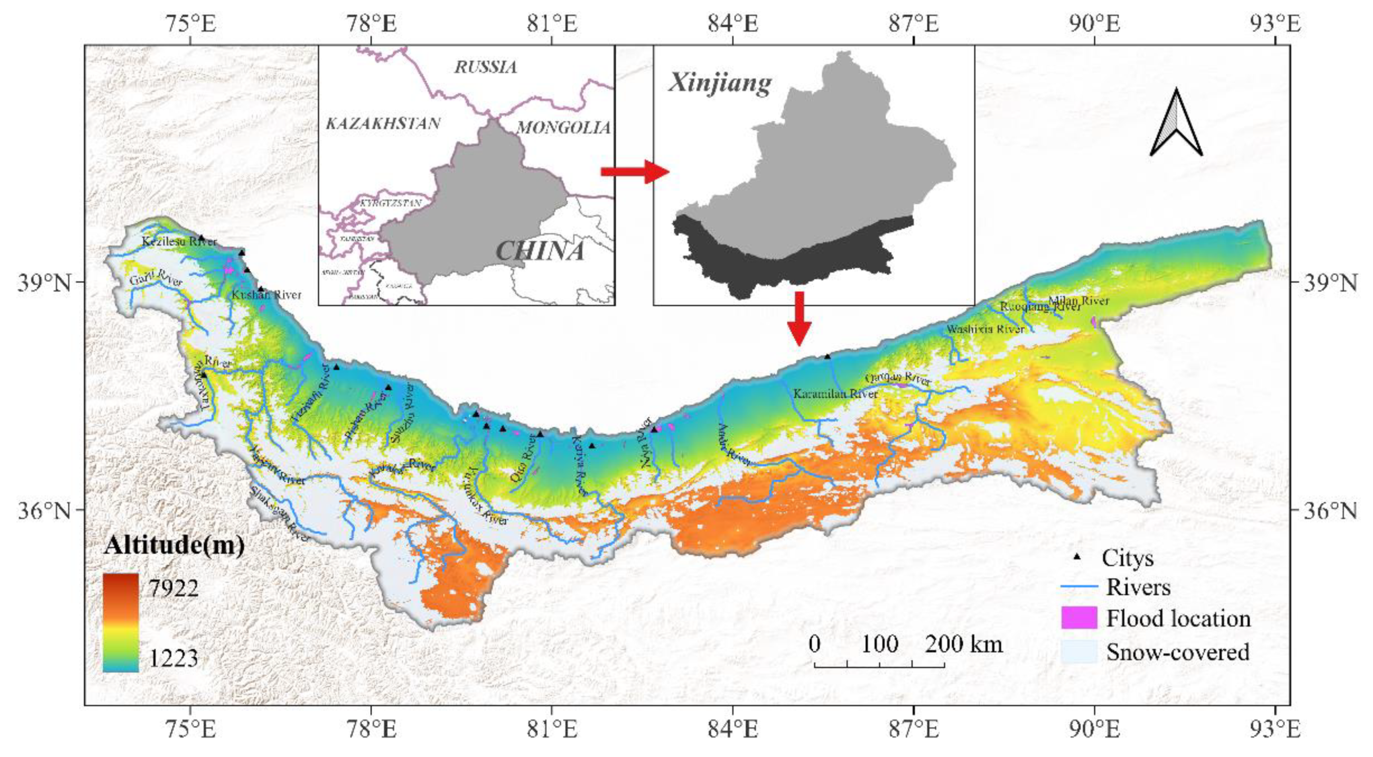
Figure 1. Locations of the study area and historical snowmelt floods.
Remotesensing 14 06360 g001
Figure 2. Conditioning factor maps: (a) aspect, (b) CI, (c) curvature, (d) distance to rivers, (e) elevation, (f) HSG, (g) land use, (h) lithology, (i) MT, (j) NDVI, (k) rainfall, (l) slope, (m) SPI, (n) STI, (o) SWE, (p) TPI, (q) TRI, (r) TWI.
Remotesensing 14 06360 g002
Figure 3. Flowchart of the proposed methodology.
Remotesensing 14 06360 g003
Figure 4. Swin Transformer structure.
Remotesensing 14 06360 g004
Figure 5. Explanation of the shift window method for calculating self-attention in the Swin Transformer architecture.
Remotesensing 14 06360 g005
Figure 6. Feature ranking based on the ReliefF method.
Remotesensing 14 06360 g006
Figure 7. ROC curve and AUC value of the (a) training set and (b) validation set.
Remotesensing 14 06360 g007
Figure 8. Snowmelt flood susceptibility in Kunlun Mountains: (a) all types, (b) mixed type and (c) warming type.
Remotesensing 14 06360 g008
Figure 9. Percentage of different susceptibility levels for different snowmelt flood types.
Remotesensing 14 06360 g009
Figure 10. Hotspot analysis results.
Remotesensing 14 06360 g010
Figure 11. Sensitivity analysis results.
Remotesensing 14 06360 g011
Table 1. Flood conditioning factors.
Factor TypeFactor NameSource of DataScale/ResolutionTime
TerrainAspectASTER GDEM Version 330 m2000
Convergence index (CI)
Curvature
Distance to rivers
Elevation
Slope
Stream power index
(SPI)
Sediment transport index (STI)
Topographic position index (TPI)
Topographic ruggedness index (TRI)
Terrain wetness index (TWI)
Meteorology
and Snow
Maximum temperature (MT)Loess Plateau Subcenter, National Earth System Science Data Center, National1 km1999–2020
RainfallScience & Technology Infrastructure of China 1999–2020
Snow water equivalent (SWE)AMSR-E/AMSR-2 product and MODIS snow cover500 m2002–2020
OthersHydrological soil group (HSG)National Cryosphere Desert Data Center, China1:1,000,0002012
LithologyGeological map of Xinjiang Uygur Autonomous Region1:5,000,0002002
Land useResource and Environment Science and Data Center, China1 km2020
Normalized difference vegetation index (NDVI)MODIS Vegetation Indices Version 6250 m2002–2020
Table 2. Hyper-parameters of models used in this study.
Model NameDescription of ParametersDetermination Framework
SVMRegularization parameter-5.5, kernel-radial basis function, gamma-0.4, seed-0, number of fold-10, batch size-64, epoch of training-100, loss function-cross entropyScikit-learn
Optuna
RFBase classifier-decision tree, max depth-4, number of trees-41, max leaf nodes-3, calc out of bag-TRUE, seed-0, number of fold-10, batch size-64, epoch of training-100, loss function-cross entropyScikit-learn
Optuna
DNNHidden layer-3, learn rate = 1.0 × 10⁻⁴, optimizer-Adam, dropout-0.5, seed-0, batch size-64, epoch of training-100, loss function-cross entropyPytorch
Optuna
CNNConvolutional layer-13, learn rate = 1.0 × 10⁻⁵, optimizer-Adam, dropout-0.5, seed-0, batch size-64, epoch of training-100, loss function-cross entropyPytorch
Optuna
Swin-TNumber of Swin-T block-24, learn rate = 1.0 × 10⁻⁶, embedding = True, optimizer-Adam, seed-0, batch size-64, epoch of training-100, loss function-cross entropyPytorch
Optuna
Table 3. The result of the multicollinearity test (VIF).
ParameterVIF ValueParameterVIF Value
Elevation7.1593SWE2.2753
Curvature3.8400Lithology2.2287
Slope3.6333Land-use1.7398
TPI3.5751TWI1.6934
TRI3.2373Distance to rivers1.6481
SPI2.8217CI1.5456
STI2.7965HSG1.3746
MT2.5249Rainfall1.3693
NDVI2.4173Aspect1.0056
Table 4. Validation results of the models using indices.
ModelTraining SetValidation Set
A (%)P (%)R (%)F (%)A (%)P (%)R (%)F (%)
Swin-T99.5599.10100.0099.5596.0795.4796.6496.05
CNN96.8394.7098.9296.7695.6293.6697.4895.53
DNN96.6494.3298.9296.5794.8692.1597.4494.72
RF93.9499.2787.4092.9691.4096.5585.6390.06
SVM88.1190.6885.0987.8084.0184.0083.4983.74
Table 5. Proportion of different snowmelt floods in each level.
Snowmelt FloodVery LowLowModerateHighVery High
All Types0.900.732.592.9092.88
Mixed Type0.080.616.219.7283.38
Warming Type0.720.956.059.2783.01
Publisher’s Note: MDPI stays neutral with regard to jurisdictional claims in published maps and institutional affiliations.