Article

Inundated Vegetation Mapping Using SAR Data: A Comparison of Polarization Configurations of UAVSAR L-Band and Sentinel C-Band

by
Abdella Salem
1 and
Leila Hashemi-Beni
2,*
1
Applied Science and Technology Program, North Carolina A&T State University, Greensboro, NC 27411, USA
2
Geomatics Program, Department of Built Environment, North Carolina A&T State University, Greensboro, NC 27411, USA
*
Author to whom correspondence should be addressed.
Remote Sens. 2022, 14(24), 6374; https://doi.org/10.3390/rs14246374
Submission received: 10 October 2022 / Revised: 7 December 2022 / Accepted: 9 December 2022 / Published: 16 December 2022
(This article belongs to the Collection Feature Paper Special Issue on Forest Remote Sensing)

Abstract

:
Flood events have become intense and more frequent due to heavy rainfall and hurricanes caused by global warming. Accurate floodwater extent maps are essential information sources for emergency management agencies and flood relief programs to direct their resources to the most affected areas. Synthetic Aperture Radar (SAR) data are superior to optical data for floodwater mapping, especially in vegetated areas and in forests that are adjacent to urban areas and critical infrastructures. Investigating floodwater mapping with various available SAR sensors and comparing their performance allows the identification of suitable SAR sensors that can be used to map inundated areas in different land covers, such as forests and vegetated areas. In this study, we investigated the performance of polarization configurations for flood boundary delineation in vegetated and open areas derived from Sentinel1b, C-band, and Uninhabited Aerial Vehicle Synthetic Aperture Radar (UAVSAR) L-band data collected during flood events resulting from Hurricane Florence in the eastern area of North Carolina. The datasets from the sensors for the flooding event collected on the same day and same study area were processed and classified for five landcover classes using a machine learning method—the Random Forest classification algorithm. We compared the classification results of linear, dual, and full polarizations of the SAR datasets. The L-band fully polarized data classification achieved the highest accuracy for flood mapping as the decomposition of fully polarized SAR data allows land cover features to be identified based on their scattering mechanisms.

1. Introduction

Flooding is one of the most frequent natural disasters that causes damage to properties, destruction to crops, and even death to humans and animals every year worldwide. In 2016, flooding affected more than 74 million people worldwide, causing 4720 deaths and more than $57 million in economic losses [1]. Global climate change causes extreme weather events that can increase flood intensity and frequency [2,3]. As climate change continues to rise, many urban and rural areas will be prone to frequent floods, especially in low-elevated coastal areas [4]. Rapid flood extent mapping helps flood relief programs and emergency management agencies to direct their resources to the most affected areas [5,6,7,8].
Floodwater extent maps have been generated from field surveys to hydrodynamic modeling to remotely sensed data [9,10,11,12,13,14]. Delineating flooded areas using field data is usually expensive and impractical [15]. Many researchers have used satellite and aerial imagery to generate floodwater extent maps. For example, [7] used optical remotely sensed data with high-resolution terrain data and social media photographs to produce rapid floodwater maps. Ban et al. analyzed optical data acquired by Terra Satellite to map floodwater along the Pampanga River in the Philippines and the Poyang and Dongting Lakes in China [16]. Despite the successful utilization of optical data for mapping open floodwater extent, it is challenging to map floodwater in forests and vegetated areas since optical sensors cannot see through clouds and underneath vegetation. Hashemi-Beni and Gebrehiwot developed an integrated method using deep learning and region growing to map the flood extent in a vegetated area using optical data [17]. While the method is promising, the quality of the floodwater map heavily relies on the quality of the topography data of the study area. Synthetic Aperture Radar (SAR) can monitor the earth’s surface day and night, independent of sunlight for illumination and in all weather conditions [18]. Due to the SAR signal capability of penetrating clouds, rain haze, and vegetation canopy, SAR provides valuable data that can be analyzed to generate near-real-time flood extent maps [19,20]. An open, calm water surface appears dark in a SAR image due to the specular reflection property of the flat water surface that reflects the SAR signal away from the SAR sensor. The presence of water underneath vegetation enhances the SAR backscattered signal due to double- and multi-bounce effects between water and vegetation structures such as trunks and stems [21]. Therefore, flooded vegetation appears bright in a SAR image.
Recently, many satellites carry onboard SAR sensors such as PALSAR-2, Sentinel-1, Radarsat-2, TerraSAR-X, and CosmoSkyMed. These SAR systems monitor the earth’s surface using various wavelengths, including X, C, and L-bands. A longer wavelength is more suitable for detecting inundated vegetation because longer wavelengths can penetrate vegetation canopy better than shorter wavelengths [5]. High temporal and spatial resolution SAR images are being used by many organizations around the world to produce near-real-time floodwater extent maps. Utilizing SAR data from various space and airborne platforms allows the production of high-temporal-resolution floodwater extent maps, especially in challenging areas like forests and vegetated areas. Inundated vegetation mapping is critical to estimate the flood extent and avoid the unseen floods that come from these areas, protecting both human life and property [17]. Before utilizing data from a SAR system, the configuration of that system, its sensor characteristics and polarization, and environmental conditions must be considered because these variables affect the reliability of floodwater extent maps [22]. Analyzing the contemporaneous data of various SAR systems acquired for the same area and comparing their results to ground reference data allows the identification of the suitable SAR system, in terms of cost and accuracy, for the particular environmental condition. Airborne SAR imagery, such as UAVSAR, can provide high spatial and temporal resolution data to monitor flooded areas in detail [5].
In contrast, satellite SAR data such as Sentinel-1b (S-1b) allows the monitoring of floodwater extent over a larger area [21]. In this study, we investigated and compared the performance of two SAR configurations (C-band and L-band) using different polarizations to detect and map floodwater extent in varying land cover types, including dense forests, short vegetation, and open areas over a flood-prone study area. To make the analyses comparable, which is a significant issue in the field of RS data analytics, and to identify promising strategies, the datasets from two important SAR systems (Sentinel 1b and NASA UAVSAR) were analyzed for the same flooding event in our study area due to Hurricane Florence in 2018.

2. Materials and Methods

2.1. Study Area and Data

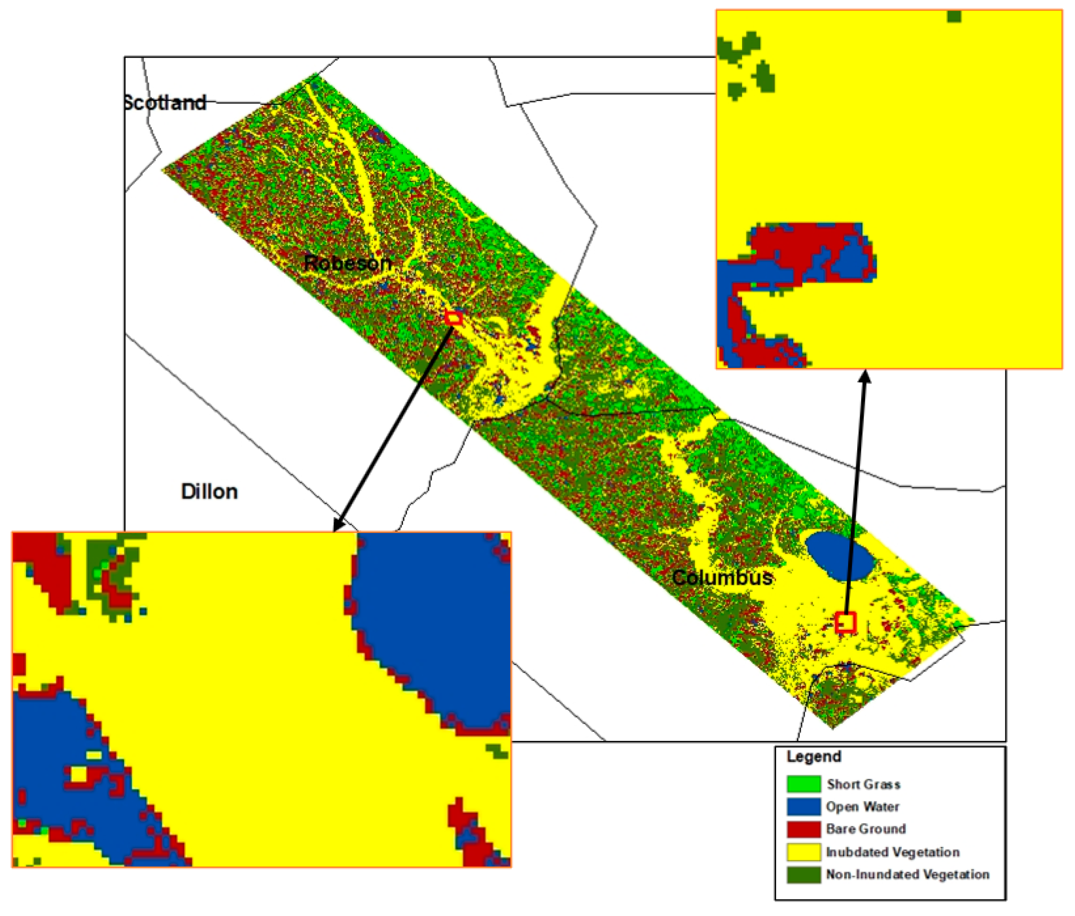
The study area was located in the eastern North Carolina coastal plain area. This area is a flood-prone area covered with dense vegetation affected by many hurricanes causing heavy rain and flooding in many counties in the state. In 2018, Hurricane Florence produced high amounts of precipitation, causing devastating flooding. Fifty-three people have been confirmed dead due to Hurricane Florence, and 77% of the causalities were in N.C.’s rural flood plain [23]. In addition, Florence was classified as one of the top 10 costliest hurricanes in United States history. As a result, FEMA identified 44 counties in the state of N.C. for federal disaster assistance. The study area is shown in Figure 1, where both UAVSAR data and S-1b SAR acquired on the same day are available.
  • UAVSAR data: The dataset includes high-resolution SAR data captured over several flight lines with repeated path observations from September 18 to 23 September 2018. UAVSAR is a fully polarized SAR system that collects data using L-band. In this study, we analyzed the ground-range-projected (GRD) format acquired over flight line 31509. These data have a pixel spacing of 6 m by 5 m.
  • Sentinel-1b: The Sentinel-1 mission contains two identical satellites: Sentinel-1a and Sentinel-1b. Each satellite provides global coverage with a revisit time of 12 days. By utilizing data from the two satellites, the global coverage temporal resolution can increase to 6 days. Sentinel-1 acquires data over the land surface using the Interferometric Wide-Swath mode with 250-km swath width and 5 × 20-m spatial resolution. Sentinel-1b collects data using dual polarization C-band (5.405 GHz, 5.6 cm wavelength), i.e., VV (vertical sent–vertical received) and VH (vertical sent–horizontal received). This research used Sentinel-1b SAR level 1 acquired on 19 September 2018 from path 77 using VV and VH polarizations.
UAVSAR data and Sentinel-1b SAR data acquired on the same date were downloaded from the Alaska Satellite Facility for the study.
  • Auxiliary data: Permanent surface water data were downloaded from the U.S. Fish and Wildlife Services National Wetland Inventory. These data were used to separate permanent open water from temporarily flooded open water and to identify permanently inundated vegetation from temporarily inundated vegetation. In addition, the research used UAV optical data to generate training and validation samples by visually identifying land cover classes. The UAV optical datasets were obtained from the National Oceanic and Atmospheric Administration.

2.2. Data Preprocessing

SAR backscattered energy is influenced by terrain variation, SAR acquisition geometry, and noise. Therefore, some data preprocessing was conducted to improve SAR data quality by reducing noise and correcting the distortions due to SAR acquisition geometry and topography variations. In addition, the preprocessing ensures that variation in SAR backscatter values is only influenced by land cover variation. Therefore, SAR preprocessing is essential for accurate land cover classifications.

2.2.1. Sentinel-1b SAR Image

The preprocessing framework of Sentinel-1b data includes (a) orbit file update, (b) border noise removal, (c) radiometric calibration, (d) speckle removal, and (f) geometric and radiometric terrain correction.
(a) Orbit file update: The orbit vector information in the metadata associated with the SAR product is created using an onboard navigation solution. The precise orbit information, including the satellite velocity and position during the image acquisition, is available by Copernicus Precise Orbit Determination (POD) Service after SAR image production. Precise orbit information is needed for data geometric and radiometric calibration.
(b) Border noise removal: The GRD level 1 production from Sentinel-1 raw data involves some processing steps. These steps include sampling start time correction to compensate for the earth’s curvature and azimuth and range compression. Unfortunately, these processes generate artifacts, including radiometric and no-value samples at the image borders [24], and the noise creates thin artifacts in the azimuth and range directions [25]. Therefore, the border noise correction eliminates low-intensity noise and invalid data on the image edges.
(c) Radiometric calibration: This step is applied to ensure that a SAR image’s pixel value directly corresponds to the radar backscatter of the sensed area. The calibration is essential for the quantitative use of level 1 SAR data. Radiometric calibration converts digital numbers in SAR image pixels to sigma naught (σ0) which is sensitive to the properties of the scattering area, incident angle, polarization, and radar wavelength [24]. The scattering coefficient (σ0) is the measure of radar-returned signal strength compared to the expected signal strength reflected by a horizontal area of a one-meter square. Sigma naught is dimensionless, usually expressed in decibels (dB), and generally computed using the pixel’s digital number (DN) and SAR sensor calibration factor (K) [26]:
σo = 10 ∗ log10(〖DN〗^2) + K
(d) Speckle removal: Speckles are noise that have a pepper appearance in SAR images. Speckles appear as the result of coherence interference between signals reflected by many elements within a resolution cell. Lee filter applies local statistics, mean, and variance of sample pixels and uses a directional window with lower mean square error [27]. In addition, the Lee filter keeps the structure in the SAR image, preserving edges and characteristic patterns associated with temporally flooded areas [26]. To remove speckles, we applied a Lee filter with a window dimension of 7 by 7.
(e) Geometric and radiometric terrain correction: SAR sensor tilt and the variation in terrain height can cause geometric distortion in SAR images. We applied the range doppler terrain correction to remove geometric terrain distortion. This method uses orbit vector information, the radar timing information in the annotation file, the slant-to-ground range conversion factor, and a reference digital elevation model (DEM) to geocode SAR images [28]. SAR image geocoding allows the location of land cover features, combining SAR data acquired by different platforms and acquisition geometry. Georeferencing is the process of rectifying SAR images to a map projection and DEM to remove distortion in SAR images caused by topography [28]. The result of the geometric correction is a geocoded SAR image with a similar geometrical representation of the sensed area. The local incident angle and topography variation influence the radar-reflected signal [26]. The terrain variations affect the brightness of the radar’s received energy which can reduce the accuracy of land cover classification [29]. The radiometric calibration implemented here was proposed by [30]:
I = (DN²/k) (sin(θ)/sin(θref))
where I is the intensity, DN is the digital number of the image, and K is the calibration constant. Then, radiometric normalization is applied using:
σ 0 corr = σ 0 sin(θ)/sin(θref)
where θ is the local incident angle, and θref is the incident angle between SAR incoming ray and normal to reference ellipsoid model of the earth’s surface.

2.2.2. UAVSAR Data

The UAVSAR processing includes (a) extraction of the coherency matrix (T3) to identify physical properties of the scattering surface, (b) speckle noise removal, (c) polarization orientation compensation, (d) T3 matrix decomposition, and (e) radiometric terrain correction and incidence angle variation effects correction.
(a) Extraction of the coherency matrix (T3).
A backscattered polarized signal from a target contains information about the target geometry, orientation, and geophysical properties. When a scattering surface reflects a SAR wave, the physical properties of the scattering surface can be extracted from the coherence matrix of the backscattered signal. The coherency matrix T represents each pixel in the polarimetric SAR image. The coherence matrix is a 3-by-3 nonnegative definite Hermitian matrix [31]:
T =   T     T   T T 12     T   T T 13 T 23 T
The coherence matrix represents the contribution of three scattering mechanisms: volume, double-bounce, and surface scattering. Comparing backscatter contributions allows retrieval of relative contribution weights of each scattering component [32].
T = PsT surface + PdT double bounce + PvT volume
where Ps, Pd, and Pv denote the power of each scattering mechanism [33].
(b) Speckle removal: Speckles are noises that appear in SAR images due to coherence interference of reflected waves from many backscatter points in the same pixel [34]. Speckles can reduce SAR image segmentation and classification accuracy [35]. We applied a 7-by-7 refined Lee filter. This filter preserves polarimetric properties and statistical correlation between channel features, edge sharpness, and point targets. The refined Lee filter applies local statistics using an edge-aligned window. Applying the Lee filter can significantly improve polarimetric SAR image classification performance [33].
(c) Polarization orientation compensation: The polarization orientation angle (POA) refers to the angle between the major axis of the polarization ellipse and the horizontal axis [35]. The POA of the scattering surface affects polarimetric SAR signature, and without the application of orientation compensation, decomposition models may produce incorrect scattering characteristics leading to misclassification. The polarization de-orientation compensates overestimation of volume scattering (especially in forest areas) that may occur due to the effects of terrain slope on the radar-backscattered signal [5].
(d) T3 coherency matrix decomposition: Decomposition techniques extract scattering mechanisms of the earth’s surface features in PolSAR data. Decomposition methods decompose total power in PolSAR image pixels into different scattering mechanisms [36]. Dominant scattering mechanisms can be identified by decomposing the T3 matrix because polarimetric SAR data are influenced by target physical properties and geometry [5]. We applied the Freeman and Durden polarimetry decompositions model. This model identifies and isolates three radar scattering mechanisms: volume scattering, double-bounce scattering, and single or odd scattering mechanisms. The result of this method is three image files representing portions of radar backscatter energy associated with each of the radar backscattering mechanisms.
(e) Radiometric terrain correction and incident angle variation effects correction: As mentioned above, terrain variation affects the brightness of SAR images even in areas with the same land cover class. Land cover signatures often become difficult to recover without terrain radiometric correction, especially in SAR image foreshortening, shadows, and layover pixels [37]. The local incident angle varies from 22 degrees in the near range to 67 degrees in the far range. This incident angle variation from near range to far range generates illumination gradients across SAR image swaths. Radar backscattered values vary with the variation in incident angle and land cover features. The UAVSAR data were radiometrically corrected for terrain and incident angle variation effects. Backscatter signatures can be misjudged without these corrections, leading to less accurate land cover classification.

2.3. Data Classification

Image classification techniques are the process of extracting information from an image to identify land cover features based on pixel values [38]. Based on the level at which image classification is performed, image classification techniques are divided into pixel-level methods and object-level methods. Pixel-level methods consider each pixel belonging to a single land cover class based on either unsupervised classification algorithms or supervised classification algorithms. The unsupervised algorithms do not require training data or prior knowledge of the study area and can identify land cover classes by clustering image values [39]. In contrast, supervised algorithms learn from training samples and label a pixel’s class by comparing its spectral information to training samples [40]. Object-level classification methods apply image segmentation techniques to divide remote sensing images into objects or geographic features and label them based on the spectral properties and other relevant measures [40].
In this study, we applied the Random Forest (RF) supervised classification algorithm. The RF classification method is fast and robust to outliers and noise [41]. RF classifiers can handle large datasets with many variables and identify important variables in the classification process [42]. RF is an ensemble classifier that generates many decision trees, and its final prediction is based on the majority of votes obtained from all trees [43]. The RF classifier builds many classification and regression trees from training data using random sampling with replacement [44]. This indicates that the same training sample can be drawn more than once, while some samples may not be drawn at all [45]. Using a random feature selection, trees are grown on a new training set without pruning [41]. Each decision tree is generated independently, and it is up to the analyst to define the number of trees and features to split each node. The RF algorithm generates decision trees with low bias and high variances [45]. One-third of the bootstrap training set is used for internal validation to evaluate the performance of the RF model [41]. It is characterized by high prediction accuracy and fast computation process [40]
Generally, decision-tree-based algorithms apply many approaches, including gain ratio, Gini index, and chi-square, to identify a suitable attribute that results in maximum dissimilarity between classes [42]. RF classifiers usually compute the Gini index to identify the characteristic that yields the best split option by measuring the impurity of the characteristics with respect to other classes [42]. Gini index is computed using the following:
J i f ( C i ,   T ) / | T | f ( C j , T ) / | T |
where T is the training sample and f (Ci, T)/|T| represents the probability of selecting pixels that belong to class Ci. In RF classification algorithms, decision trees are extended to their full depth without pruning using a combination of variables or features. As a result, the RF classifier is more advanced than other decision-based methods because the performance of tree-based classification methods is affected by the choice of pruning approaches and not attribute selection measures [43]. The computation time needed to build the RF classification model can be computed using the following [41]:
T M N l o g N
where T represents the number of trees, M is the number of features or variables used in node split, and N is the size of training samples.
The classification process includes (a) land cover sample labeling and (b) training, prediction, and validation.
(a) Land cover sample labeling
The UAV high-resolution optical data were overlaid with SAR data. We visually identified five different land cover types: open water, bare ground, grassland, inundated vegetation, and non-inundated vegetation. Over 120 training samples for each of the five land covers were manually annotated.
(b) Training, prediction, and validation
Supervised classification methods require training samples selected from sites with known land cover types to represent land cover classes in the area of interest. Supervised classifiers compare the spectral information of image pixels with the spectral pattern in the training samples. Then, some statistical and classification decision rules are used to assign each image pixel to a class with the highest similarity to the pixel [40]. Ground truth data are generally used to assess the accuracy of the classifier. In this study, we randomly selected 75% of the training sample pixels for training, and 25% of the samples were withheld for validation. This process generated 214,572 point samples for training and 7143 points for validation for the S-1b data. For The UAVSAR data, 51,980 and 17,182 point samples were randomly selected for training and validation of the predictions. The RF classifier was trained using the selected training sample pixels for each land cover type. Various numbers of decision trees and variables per split were tested. The model with 300 trees and 3 variables per split has achieved high training accuracy, so we classified the data using this model.

3. Results

The classification accuracy was estimated using validation samples, i.e., the annotated data that had not been seen by the RF classifier.

3.1. UAVSAR L-Band Classification Results

The UAVSAR data was classified using three models: linear polarization (VV/VH), dual polarization, and full polarization.
(a) L-band linear polarization: The linear polarizations VV and VH were analyzed and segmented using the RF method to create a flood map of the study areas. The performance of the classification results was evaluated using a confusion matrix representing counts from predicted and actual values in the classifications. The confusion matrix of this VV model is shown in Table 1, which was generated by comparing the land cover classification results obtained from this model to the training samples.
After generating the confusion matrix, we computed the training accuracy using:
O v e r a l l   t r a i n i n g   A c c u r a c y   ( O A ) = t o t a l   n u m b e r   o f   c o r r e c t l y   c l a s s i f i e d   p i x e l s t o t a l   n u m b e r   o f   p i x e l s   i n   t h e   t r a i n g   s a m p l e O A   f o r   t h e   V V   M o d e l = 22 , 124 22 , 346   = 99.01 %
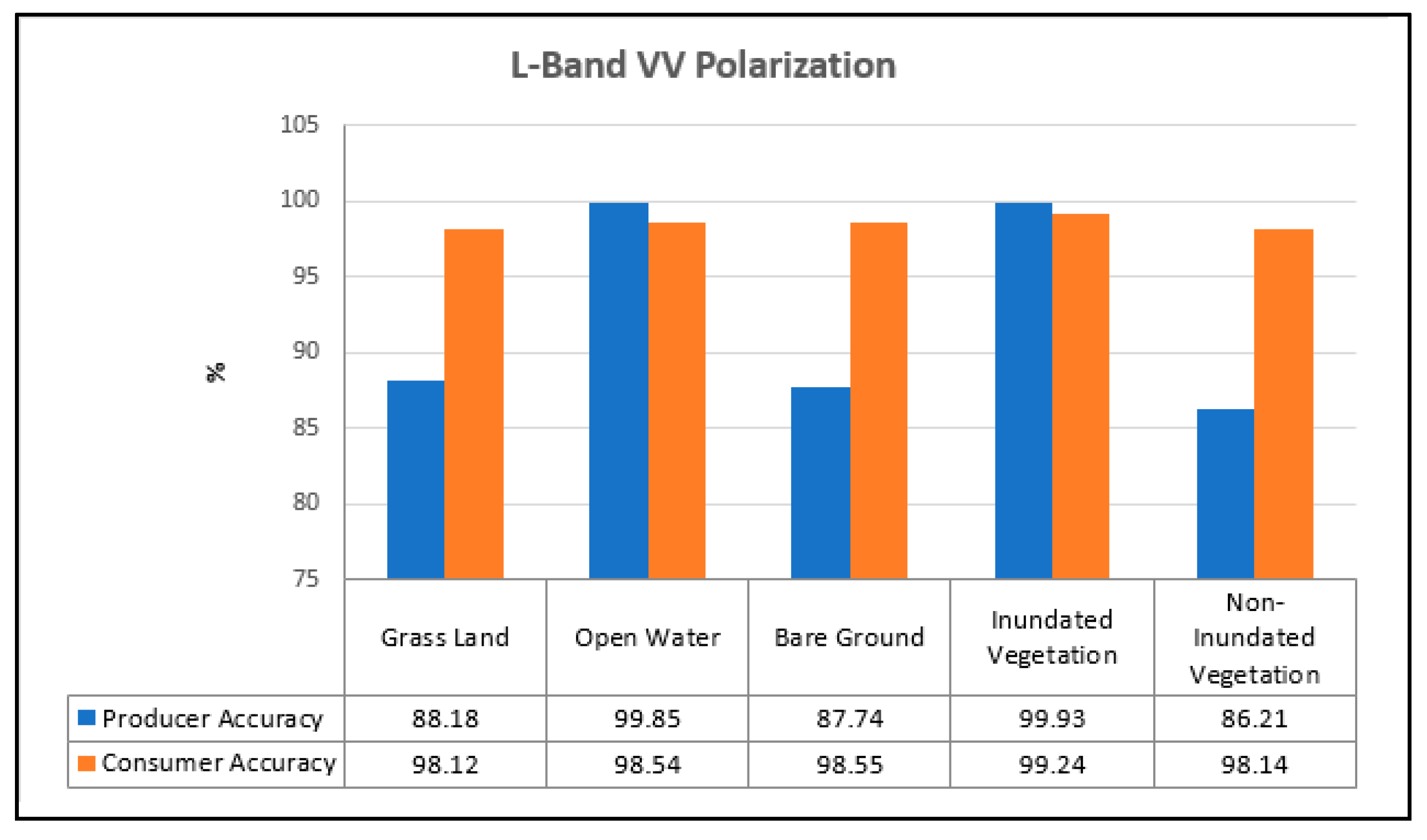
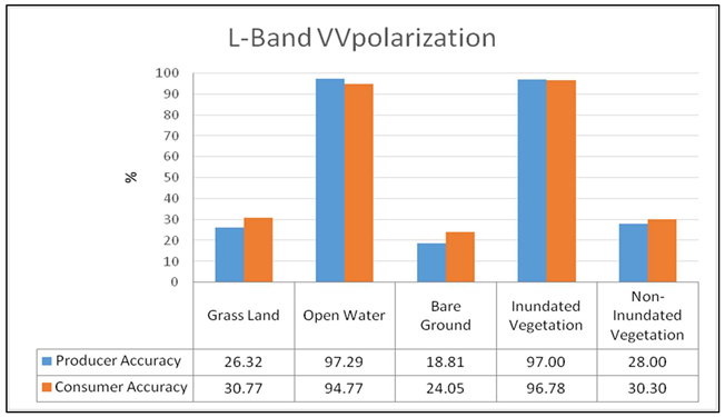
The producer and consumer accuracy for the UAVSAR VV model is shown in Figure 2. The classification accuracy was also evaluated using kappa statistics. Kappa statistics provide additional accuracy assessment measuring test interrater reliability. Kappa statistic (k) is calculated by subtracting the summation of chance agreement from the summation of the agreement of the results [44].
K = ( P o b P c ) ( 1 P c h )
where Po is observed agreement, and Pch is the chance agreement. K for UAV training:
P o b = ( 418 22,346 ) + ( 5487 22,346 ) + ( 272 22,346 ) + ( 15,259 22,346 ) + ( 688 22,346 ) = 0.9901 P c h = [ ( 474 426 22,346 ) + ( 5495 5568 22,346 ) + ( 310 276 22,346 ) + ( 15,269 15,375 22,346 ) + ( 798 701 22,346 ) ] / 22,346 = 0.53 K = ( 0.9901 0.5331 ) ( 1 0.5331 ) = 97.88 %
The validation error matrix for the classification of the UAVSAR VV polarization data was generated by comparing the classification results with the reference data samples that the classifier has not seen, hence providing a reliable accuracy assessment. The overall validation accuracy for this model is 92.35%, with kappa statistics of 83.65%. The validation error matrix for this model is shown in Table 2.
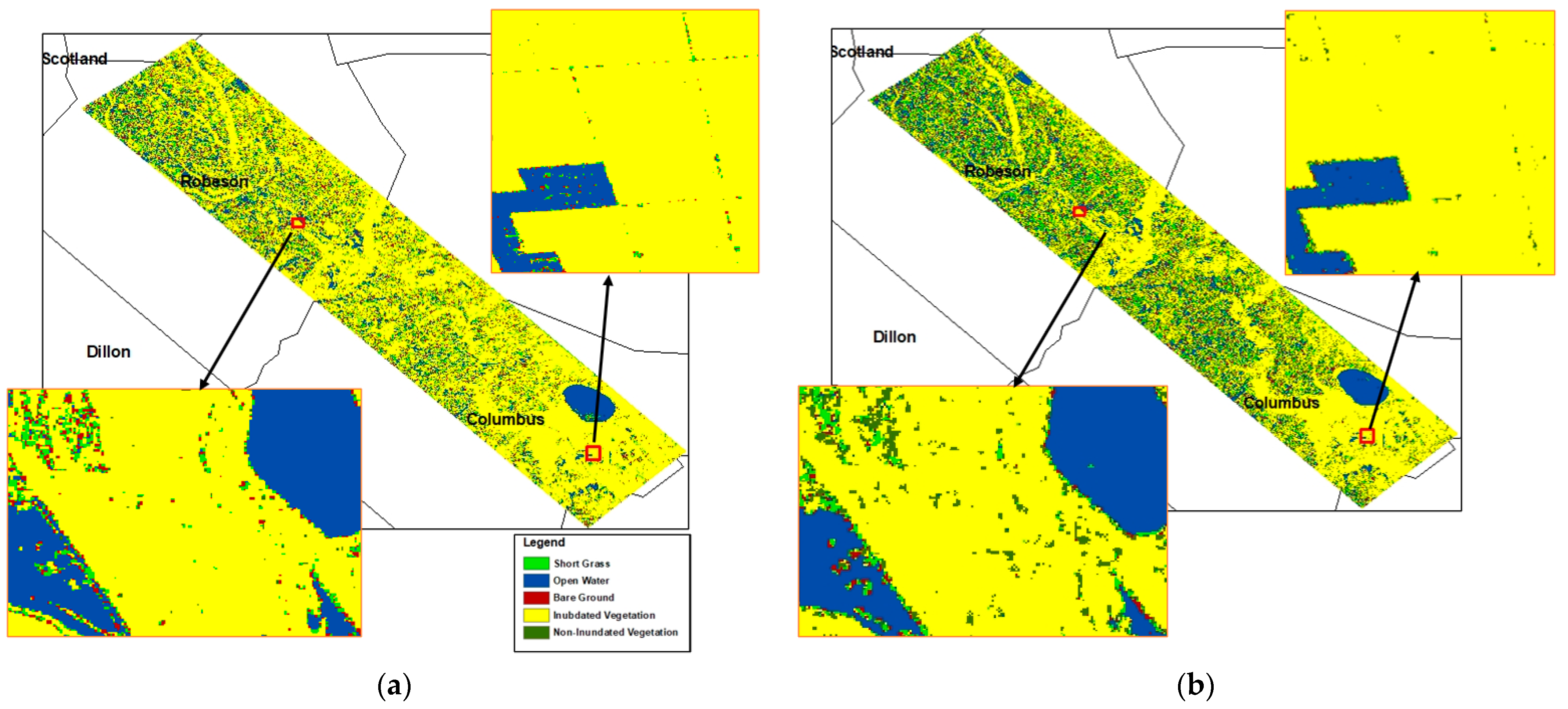
The linear polarization of VH was also analyzed and segmented using the RF method to create a flood map of the study areas. The results of the classification are described in Figure 3 and Figure 4.
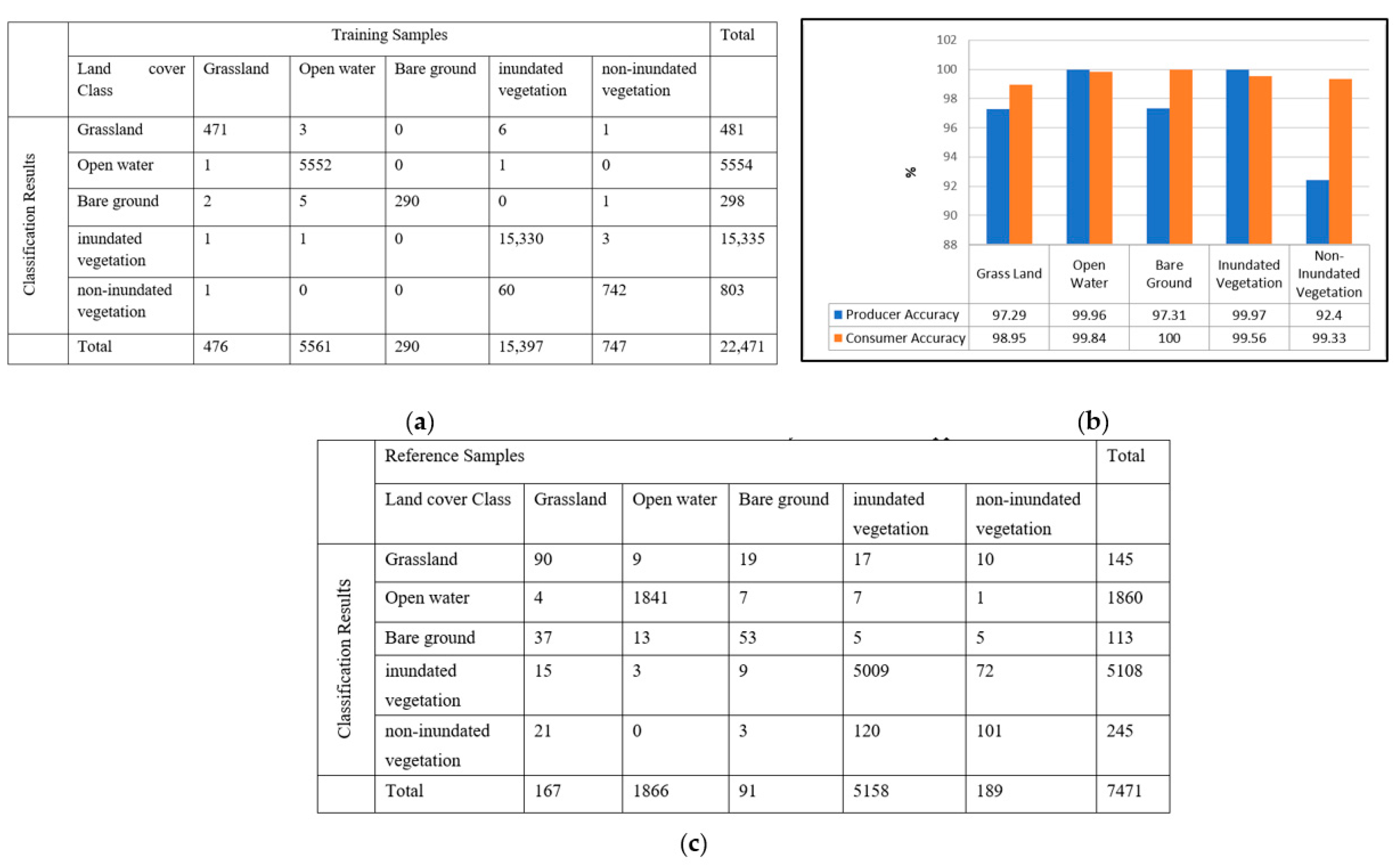
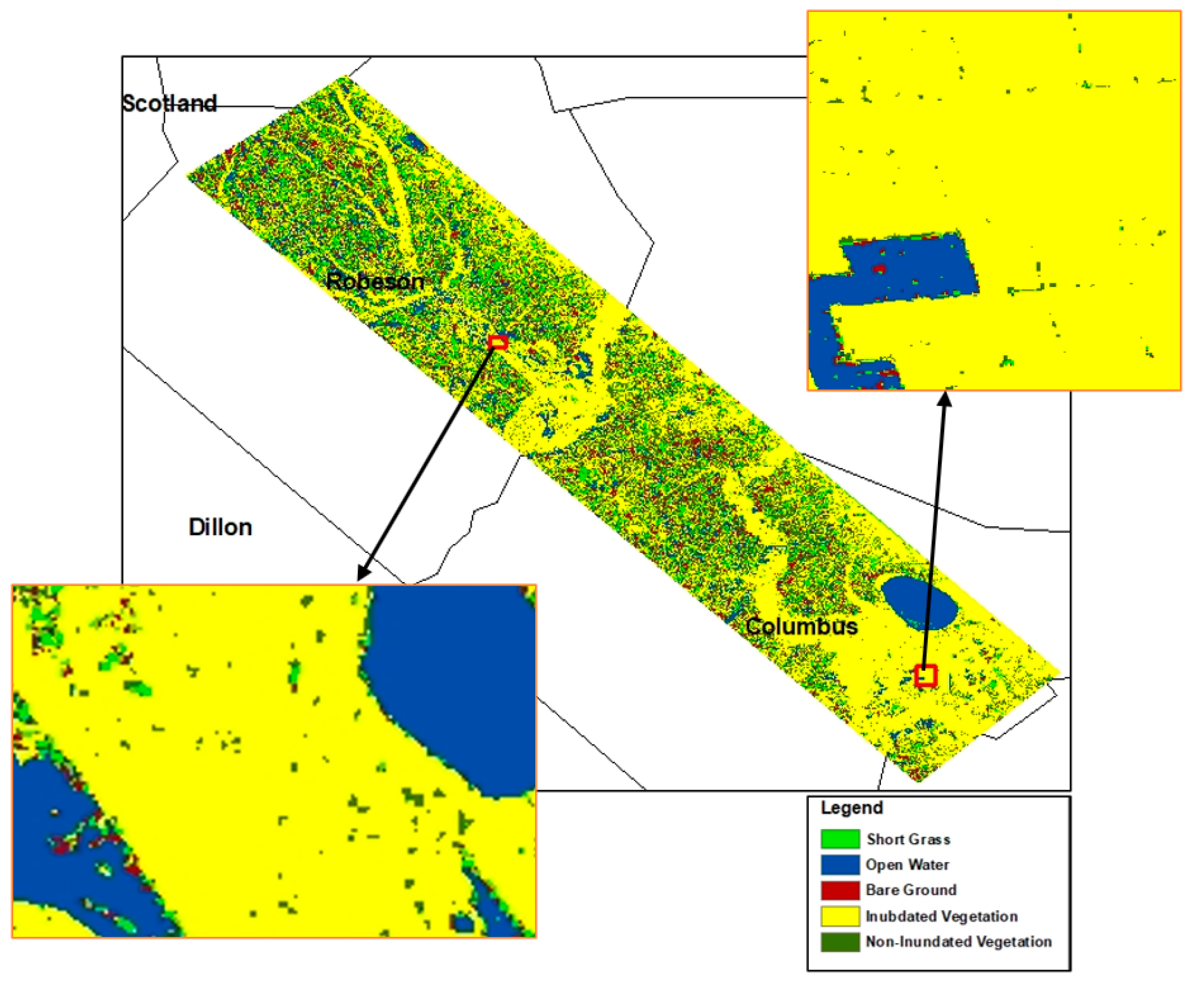
(b) L-band dual polarization: To study the performance of the UAVSAR dual polarization for flood mapping, a composite image was created using the VV, VH, and the ratio |VV|/|VH|. This image was classified using the RF classification algorithm. Figure 5 describes the classification performance for the training and validation of the L-band dual polarization for flood mapping. This model has an overall training accuracy of 99.61% with a kappa coefficient of 99.18. The validation error samples for this model are shown in Figure 5 and Figure 6. This model shows overall validation accuracy of 94.95%, with kappa statistics of 89.13%.
(c) L-band full polarization: This study also utilized the UAVSAR full polarization for flood mapping. The performance of the UAVSAR data classification is described in Figure 7 and Figure 8.
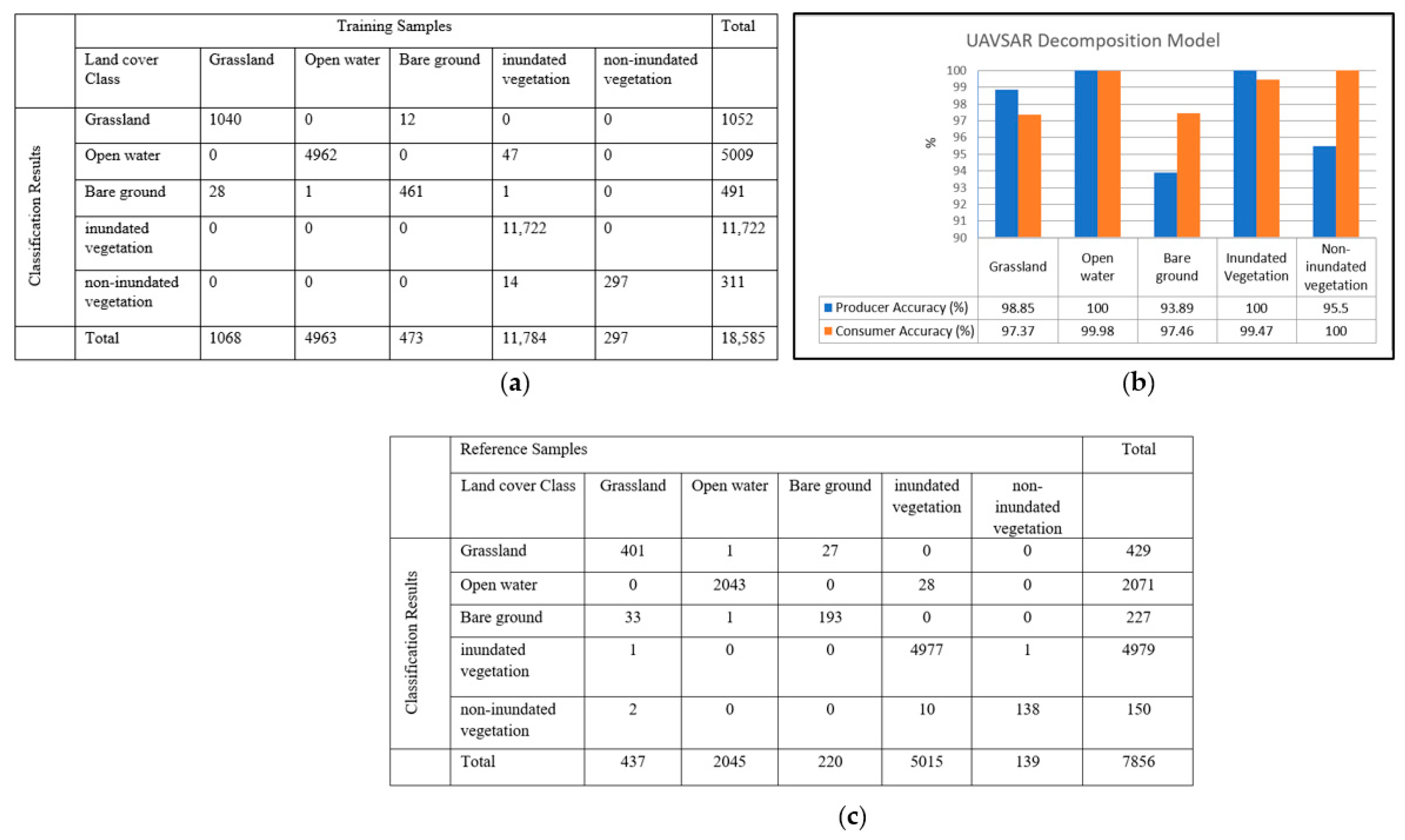
The overall training accuracy and validation accuracy for the UAVSAR decomposition model are 99.45% and 98.68%, respectively. The kappa statistic for the validation reference samples is 97.47%.

3.2. Sentinel C-Band Classification Results

We also generated the confusion matrices for the classification results obtained from S-1b linear polarization (i.e., VV and VH) and dual polarization by comparing the classifier outputs to training samples.
(a) C-band linear polarization: The linear polarizations from sentinel C-band VV- and VH-polarized data were analyzed and segmented using the RF method to create a flood map of the study areas. The performance of the classification results was evaluated using a confusion matrix representing counts from predicted and actual values in the classifications. The performance of the S-1b VV and VH data classification is described in Figure 9 and Figure 10.
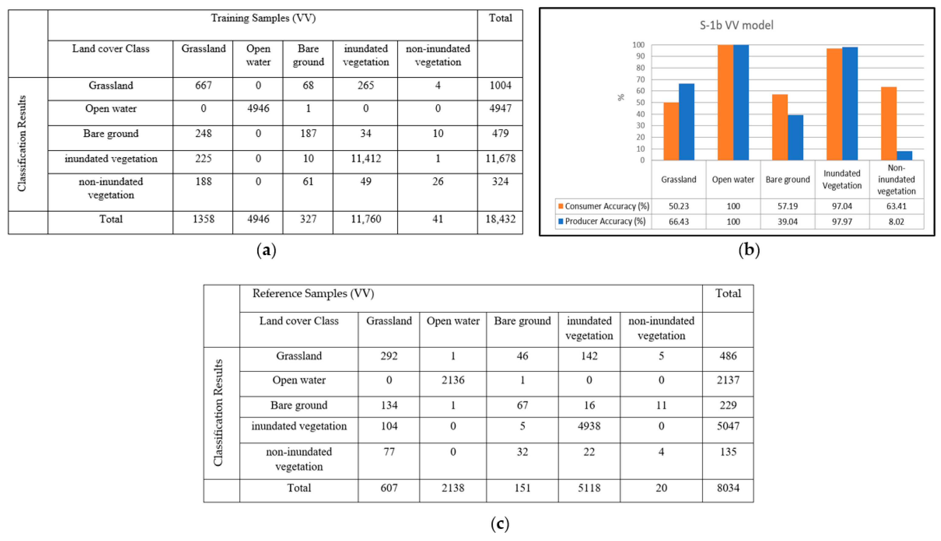
The overall training accuracy for the S-1bVVSAR model is 93.52% (17,238/18,432). The kappa statistic for the overall training accuracy is 87.81%. The VV model producer and consumer accuracy are shown in Figure 9b. We noticed that the model predicted open water and inundated vegetation very well. However, for non-inundated vegetation, the model showed low producer accuracy. The validation error matrix for the S-1b (VV) model is shown in Figure 10c. The overall validation accuracy for the S-1b SAR VV model is 92.57% (7437/8034), and the kappa statistic for the validation accuracy is 85.81%.
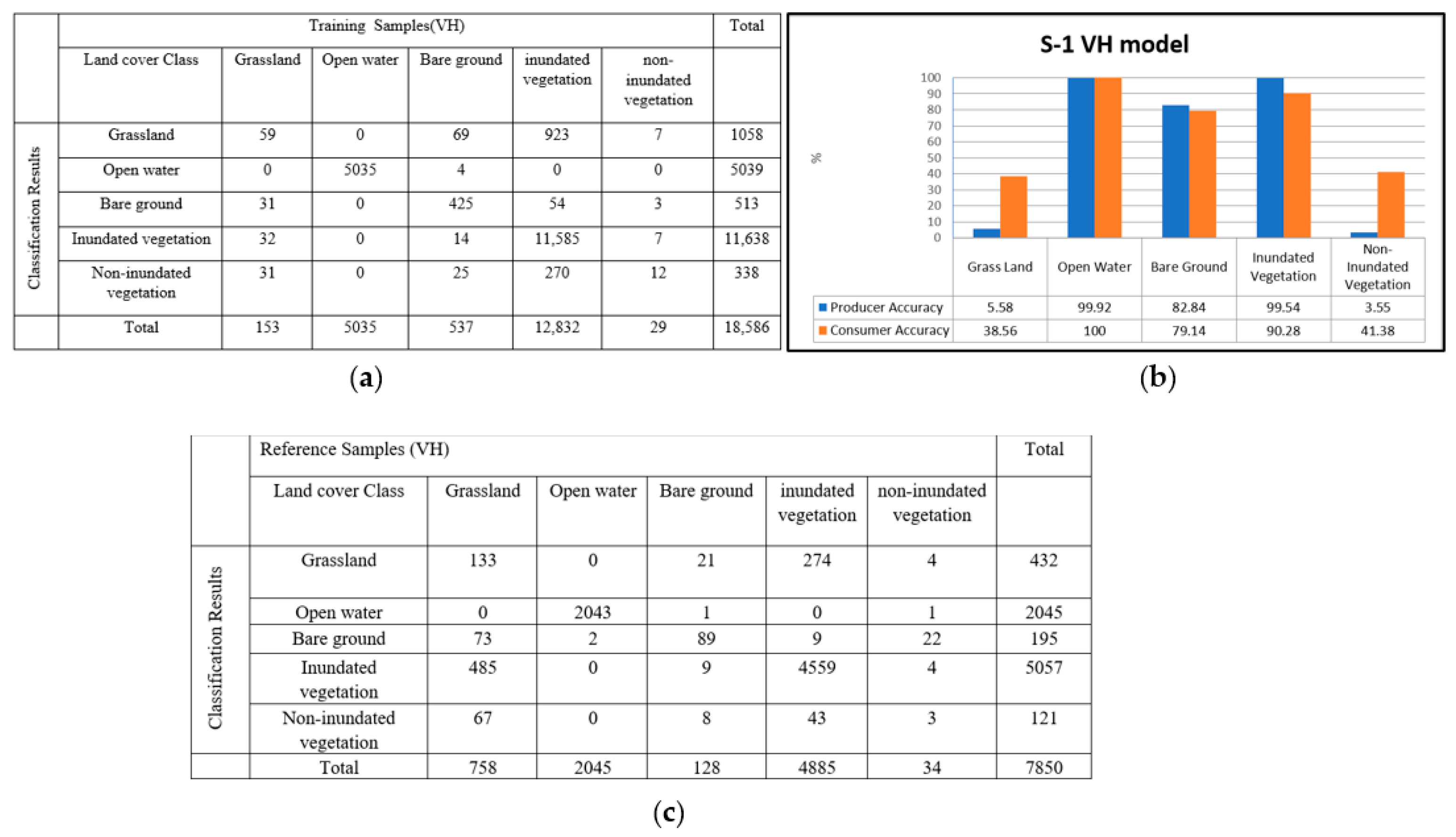
The overall accuracy for the S-1b SAR data (VH polarization) is 86.97% (6827/7850). This model also predicted open water and inundated vegetation with high accuracy (Figure 11). The S-1b VH model overall validation accuracy had a kappa statistic of 75.2%.
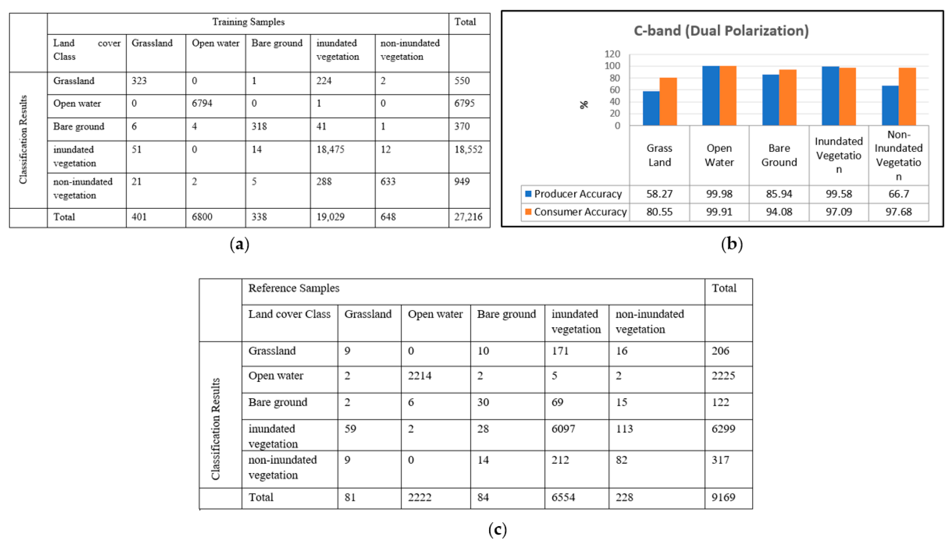
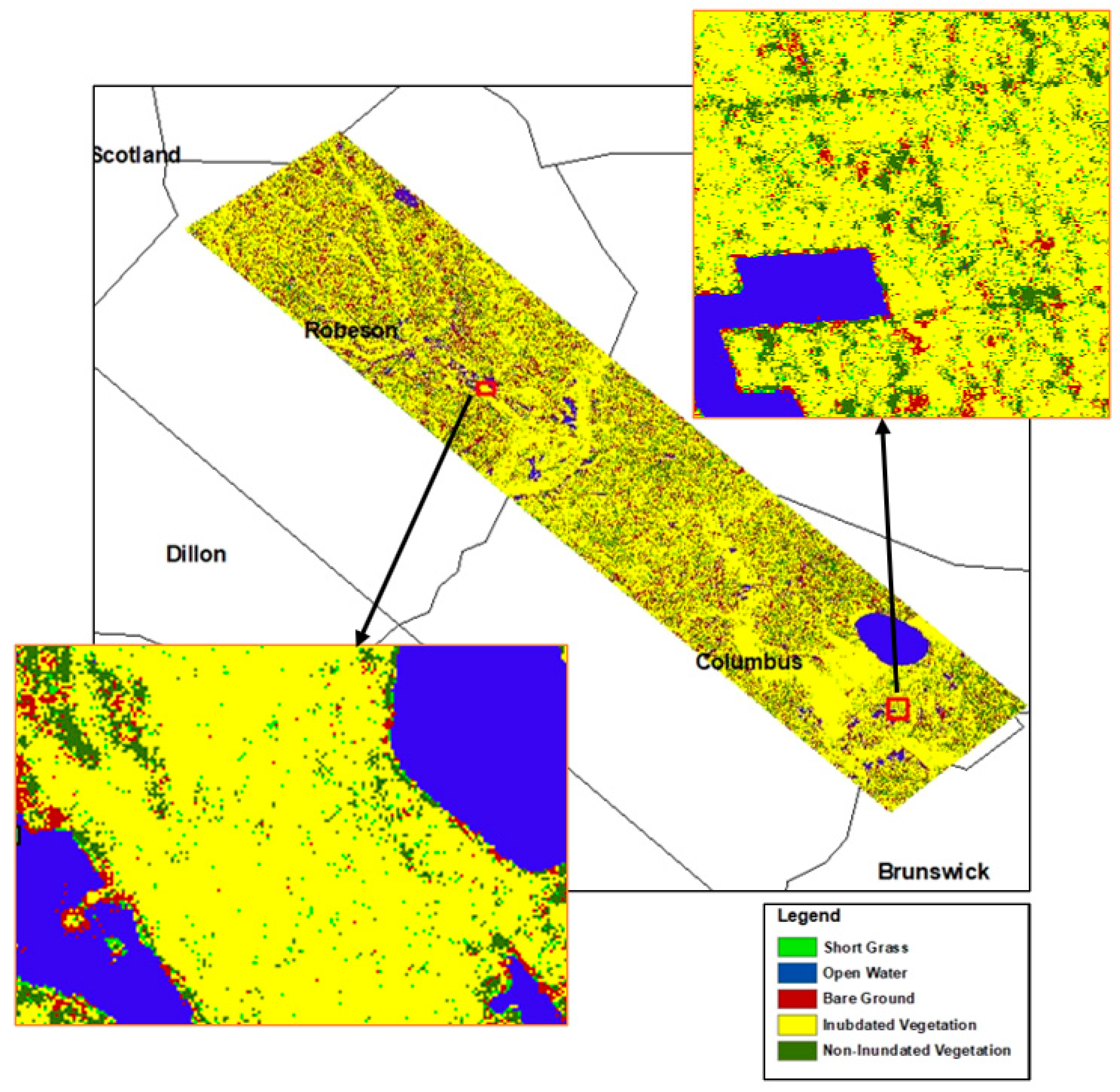
C-band dual polarization: Similar to the UAVSAR dual polarization analysis for flood mapping, a composite image was created using the Sentinel C-band VV, VH, and the ratio |VV|/|VH|. This image was classified using the RF classification algorithm. Figure 12 shows the classification performance for the training and validation of the C-band dual-polarized data for flood mapping. This model has an overall training accuracy of 97.53% with a kappa coefficient of 94.61%. The validation error samples for this model are shown in Figure 12c. This model has an overall validation accuracy of 91.96%, with kappa statistics of 82.01% (Figure 13).
Table 3 summarizes the training and validation accuracy of the RF classification of the UAVSAR L-band and Sentinel 1b C-band for flood mapping using different polarization configurations.
We noticed that both Sentinel and UAVSAR datasets accurately predicted open water areas as expected, because of the high contrast between an open water surface and other land cover features in the study area. This high contrast results from the specular reflection property of calm open water surfaces, causing radar signals to be reflected away from the SAR antenna and making pixels of open water appear dark in the SAR datasets. In addition, some inundated vegetated areas that appeared bright in the SAR images were also accurately detected. The presence of water underneath vegetation enhanced the SAR backscattered signal due to double-bounce and multi-bounce effects between flat water surfaces and vertical vegetation structures, such as trunks and stems, leading to the higher prediction accuracy of inundated vegetation pixels.
The results show that co-polarization VV performed slightly better than the cross-polarization VH for floodwater mapping using both L-band and C-band. As expected, the combination of L-band SAR polarizations (dual and full polarization) performed better than retrieving the floodwater class from a single polarization. However, the classification of the S-1b C-band dual polarization did not increase the flood map accuracy more than the results obtained from the co-polarization of VV. Because the L-band penetrates the vegetation canopy better than the C-band, the overall accuracy of the L-band dual-polarized data was higher than that of the C-band dual-polarized data. The L-band fully polarized data classification achieved the highest accuracy for flood mapping because the decomposition of fully polarized SAR data allows land cover features to be identified based on their scattering mechanisms.
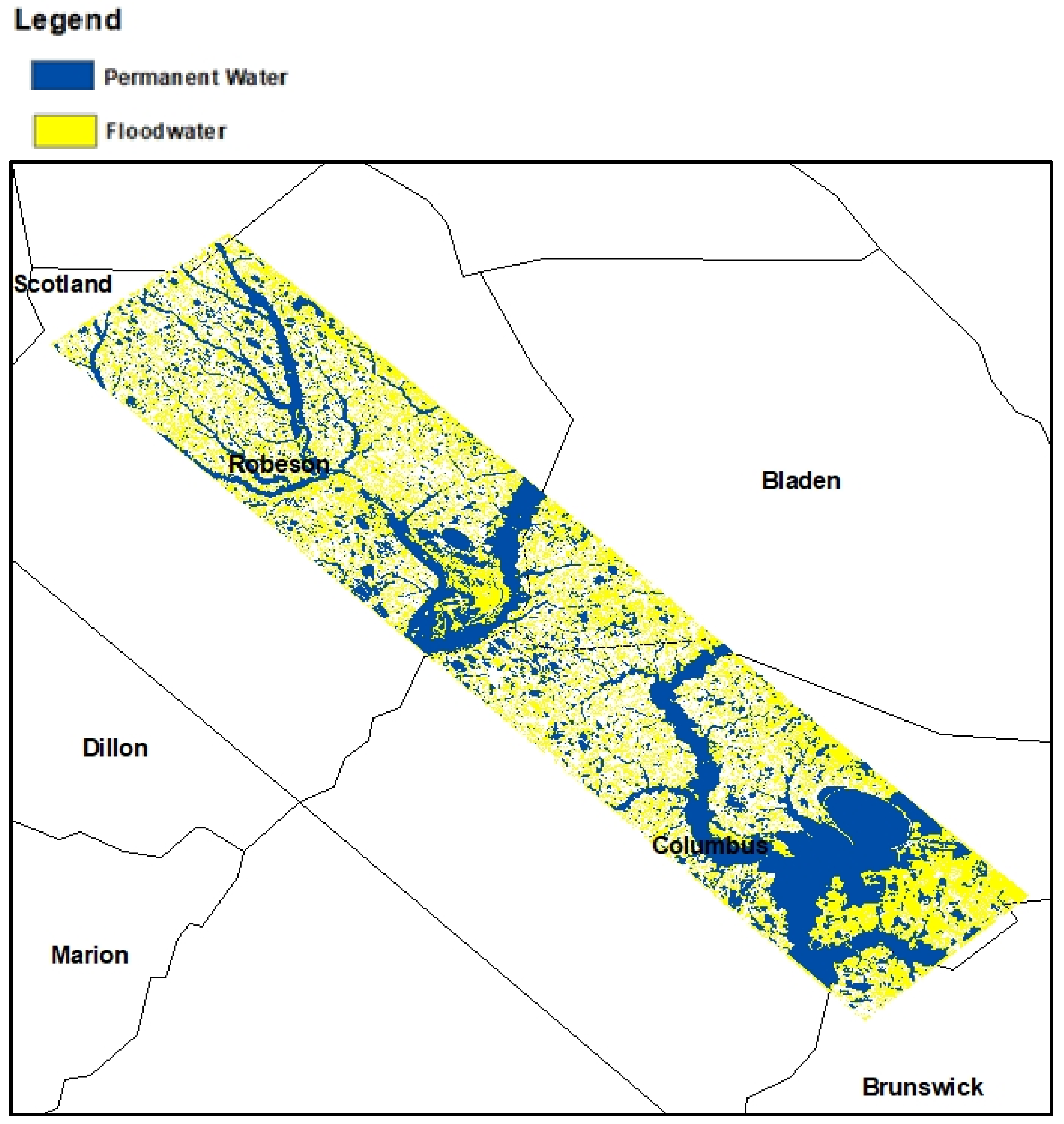
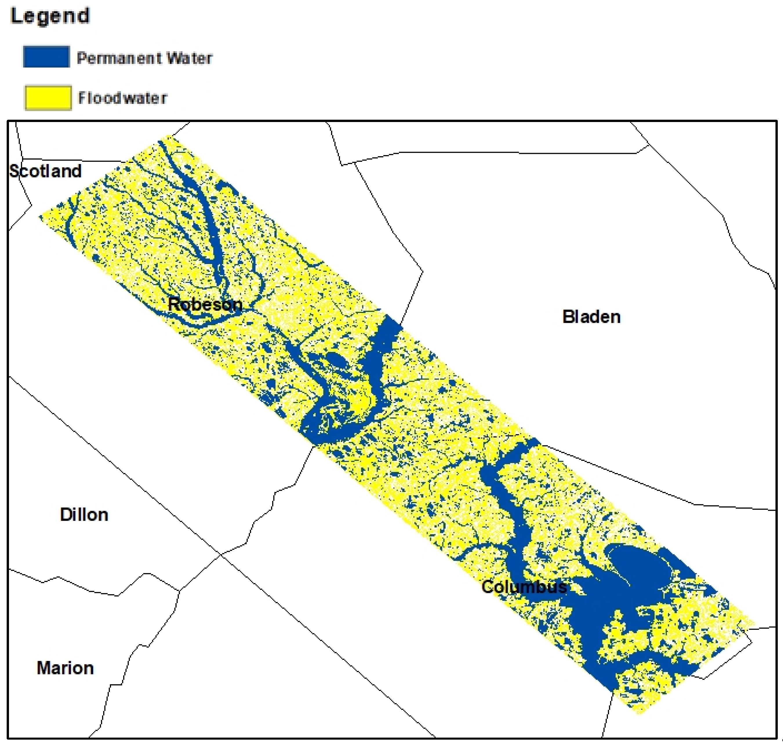
Finally, the flooded vegetation and open floodwater areas were identified by masking permanent water areas. The permanent water layers over our study area, including water under vegetation and open water, were obtained from US fish and wildlife services. The floodwater, including both inundated vegetation and open floodwater detected by UAVSAR and S-1b SAR dual-polarized datasets, are shown in Figure 14 and Figure 15, respectively.

4. Conclusions

Inundated vegetation mapping is critical to estimate the flood extent and avoid the unseen floods that come from these areas, thus protecting both human life and property. This study investigated the performance of different polarization configurations of UAVSAR L-band and Sentinel C-band datasets for inundated vegetation mapping over a flood-prone study area in North Carolina (USA) during Hurricane Florence. Both datasets were suitable for predicting open water with high accuracy. The forward reflection characteristics associated with calm, open water bodies result in low radar backscatter values causing high contrast between open water and other land cover features, leading to the accurate identification of pixels of open water areas. However, inundated vegetation pixels exhibit the double-bounce scattering mechanism identified when decomposing the coherence matrix of fully polarized L-band SAR data. This helps predict flooded vegetation with high accuracy since L-band signals penetrate vegetation canopies more than C-band. The overall floodwater classification accuracy obtained from the Freeman–Durden decomposition of fully polarized L-band reached 98.68%. In addition, the Freeman–Durden decomposition model of the fully polarized SAR data identifies different scattering mechanisms corresponding to different land cover classes, improving the accuracy of the land cover classification.
The backscattered signal enhancement due to double- and multi-bounce effects between the flat water surface and vertical vegetation structures helped identify inundated vegetation with high accuracy. The S-1b VV model had an overall accuracy of 92.57%, while the S-1bVH model achieved 86.97% overall classification accuracy. Therefore, sentinel data showed promising performance in predicting inundated vegetation in the area. Our results showed that the S-1b co-polarization performed slightly better than the S-1b cross-polarization, which agrees with previous studies [46,47,48]. However, our results showed that the S-1b C-band dual polarization did not increase the flood map accuracy more than the results obtained from the co-polarization VV. Therefore, the VV-polarized data from Sentinel 1b are suitable for mapping inundated vegetation in large study areas with reasonable accuracy. In addition, satellite data allow the monitoring of regional floodwater mapping with less cost than airborne SAR datasets.

Author Contributions

Conceptualization, A.S. and L.H.-B.; methodology, A.S. and L.H.-B.; software, A.S.; validation, A.S. and L.H.-B.; formal analysis, A.S. and L.H.-B.; investigation, L.H.-B. and A.S.; resources, L.H.-B.; data curation, A.S.; writing—original draft preparation, A.S. and L.H.-B.; writing—review and editing, A.S. and L.H.-B.; visualization, A.S.; supervision, L.H.-B.; project administration, L.H.-B.; funding acquisition, L.H.-B. All authors have read and agreed to the published version of the manuscript.

Funding

Partial funding for the study was provided by NOAA award #NA21OAR4590358 and by the National Science Foundation under Grant No. 1800768.

Data Availability Statement

Not applicable.

Conflicts of Interest

The authors declare no conflict of interest.

References

  1. Paterson, D.L.; Wright, H.; A Harris, P.N. Health risks of flood disasters. Clin. Infect. Dis. 2018, 67, 1450–1454. [Google Scholar] [CrossRef] [PubMed] [Green Version]
  2. Slater, L.J.; Villarini, G. Recent trends in U.S. flood risk. Geophys. Res. Lett. 2016, 43, 12. [Google Scholar] [CrossRef] [Green Version]
  3. Esposito, G.; Matano, F.; Scepi, G. Analysis of increasing flash flood frequency in the densely urbanized coastline of the campi flegrei volcanic area, Italy. Front. Earth Sci. 2018. [Google Scholar] [CrossRef]
  4. Zhao, J.; Pelich, R.; Hostache, R.; Matgen, P.; Cao, S.; Wagner, W.; Chini, M. Deriving exclusion maps from C-band SAR time-series in support of floodwater mapping. Remote Sens. Env. 2021, 265, 112668. [Google Scholar] [CrossRef]
  5. Wang, C.; Pavelsky, T.M.; Yao, F.; Yang, X.; Zhang, S.; Chapman, B.; Song, C.; Sebastian, A.; Frizzelle, B.; Frankenberg, E.; et al. Flood extent mapping during Hurricane Florence with repeat-pass L-band UAVSAR images. ESS Open Arch. 2021. [Google Scholar] [CrossRef]
  6. Li, Y.; Martinis, S.; Plank, S.; Ludwig, R. An automatic change detection approach for rapid flood mapping in Sentinel-1 SAR data. Int. J. Appl. Earth Obs. Geoinf. 2018, 73, 123–135. [Google Scholar] [CrossRef]
  7. Rosser, J.F.; Leibovici, D.G.; Jackson, M.J. Rapid flood inundation mapping using social media, remote sensing and topographic data. Nat. Hazards 2017, 87, 103–120. [Google Scholar] [CrossRef] [Green Version]
  8. Manjusree, P.; Kumar, L.; Bhatt, C.M.; Rao, G.S.; Bhanumurthy, V. Optimization of threshold ranges for rapid flood inundation mapping by evaluating backscatter profiles of high incidence angle SAR images. Int. J. Disaster Risk Sci. 2012, 3, 113–122. [Google Scholar] [CrossRef] [Green Version]
  9. Gebrehiwot, A.; Hashemi-Beni, L.; Thompson, G.; Kordjamshidi, P.; Langan, T.E. Deep convolutional neural network for flood extent mapping using unmanned aerial vehicles data. Sensors 2019, 19, 1486. [Google Scholar] [CrossRef] [Green Version]
  10. Hashemi-Beni, L.; Gebrehiwot, A. Deep learning for remote sensing image classification for agriculture applications. Int. Arch. Photogramm. Remote. Sens. Spat. Inf. Sci. 2020, XLIV-M-2-2, 51–54. [Google Scholar] [CrossRef]
  11. Anusha, N.; Bharathi, B. Flood detection and flood mapping using multi-temporal synthetic aperture radar and optical data. Egypt. J. Remote. Sens. Space Sci. 2020, 23, 207–219. [Google Scholar] [CrossRef]
  12. Gebrehiwot, A.; Hashemi-Beni, L. Automated Indunation Mapping: Comparison of Methods. In Proceedings of the IGARSS 2020-2020 IEEE International Geoscience and Remote Sensing Symposium, Waikoloa, HI, USA, 26 September–2 October 2020; pp. 3265–3268. [Google Scholar]
  13. Gebrehiwot, A.; Hashemi-Beni, L. A Method to Generate Flood Maps in 3d Using dem and Deep Learning. ISPRS Int. Arch. Photogramm. Remote Sens. Spat. Inf. Sci. 2020, 44, 1800768. [Google Scholar] [CrossRef]
  14. Beni, L.H.; Jones, J.; Thompson, G.; Johnson, C.; Gebrehiwot, A. Challenges and Opportunities for UAV-Based Digital Elevation Model Generation for Flood-Risk Management: A Case of Princeville, North Carolina. Sensors 2018, 18, 3843. [Google Scholar] [CrossRef] [Green Version]
  15. Brakenridge, R.; Anderson, E. MODIS-based flood detection, mapping and measurement: The potential for operational hydrological applications. In Transboundary Floods: Reducing Risks Through Flood Management; Kluwer Academic Publishers: Dordrecht, The Netherlands, 2006; pp. 1–12. [Google Scholar] [CrossRef]
  16. Ban, H.-J.; Kwon, Y.-J.; Shin, H.; Ryu, H.-S.; Hong, S. Flood monitoring using satellite-based RGB composite imagery and refractive index retrieval in visible and near-infrared bands. Remote Sens. 2017, 9, 313. [Google Scholar] [CrossRef] [Green Version]
  17. Hashemi-Beni, L.; Gebrehiwot, A.A. Flood extent mapping: An integrated method using deep learning and region growing using UAV optical data. IEEE J. Sel. Top. Appl. Earth Obs. Remote. Sens. 2021, 14, 2127–2135. [Google Scholar] [CrossRef]
  18. Colesanti, C.; Wasowski, J. Investigating landslides with space-borne Synthetic Aperture Radar (SAR) interferometry. Eng. Geol. 2006, 88, 173–199. [Google Scholar] [CrossRef]
  19. Rahman, M.R.; Thakur, P.K. Detecting, mapping and analysing of flood water propagation using synthetic aperture radar (SAR) satellite data and GIS: A case study from the Kendrapara District of Orissa State of India. Egypt. J. Remote Sens. Space Sci. 2018, 21, S37–S41. [Google Scholar] [CrossRef]
  20. Liang, J.; Liu, D. A local thresholding approach to flood water delineation using Sentinel-1 SAR imagery. ISPRS J. Photogramm. Remote. Sens. 2019, 159, 53–62. [Google Scholar] [CrossRef]
  21. Tsyganskaya, V.; Martinis, S.; Marzahn, P. Flood monitoring in vegetated areas using multitemporal sentinel-1 data: Impact of time series features. Water 2019, 11, 1938. [Google Scholar] [CrossRef]
  22. Tsyganskaya, V.; Martinis, S.; Marzahn, P.; Ludwig, R. SAR-based detection of flooded vegetation–a review of characteristics and approaches. Int. J. Remote Sens. 2018, 39, 8. [Google Scholar] [CrossRef]
  23. Paul, S.; Ghebreyesus, D.; Sharif, H.O. Brief Communication: Analysis of the fatalities and socio-economic impacts caused by hurricane florence. Geosciences 2019, 9, 58. [Google Scholar] [CrossRef] [Green Version]
  24. Filipponi, F. Sentinel-1 GRD preprocessing workflow. Proceedings 2019, 18, 11. [Google Scholar] [CrossRef] [Green Version]
  25. Luo, Y.; Flett, D. Sentinel-1 Data Border Noise Removal and Seamless Synthetic Aperture Radar Mosaic Generation. Proceedings 2018, 2, 330. [Google Scholar] [CrossRef] [Green Version]
  26. Rosenqvist, A.; Killough, B. A Layman’s Interpretation Guide to L-Band and C-band Synthetic Aperture Radar Data; Comittee on Earth Observation Satellites: Washington, DC, USA, 2018. [Google Scholar]
  27. Medasani, S.; Reddy, G.U. Analysis and Evaluation of Speckle Filters by Using Polarimetric Synthetic Aperture Radar Data Through Local Statistics. In Proceedings of the 2nd International Conference on Electronics, Communication and Aerospace Technology, ICECA, Coimbatore, India, 29–31 March 2018; pp. 169–174. [Google Scholar] [CrossRef]
  28. Guide to S-1 Geocoding Guide to Sentinel-1 Geocoding. Sentinel-1 Mission Performance Center. 2022. Available online: https://sentinel.esa.int/documents/247904/3976352/Guide-to-Sentinel-1-Geocoding.pdf/e0450150-b4e9-4b2d-9b32-dadf989d3bd3 (accessed on 19 May 2022).
  29. Small, D. Flattening gamma: Radiometric terrain correction for sar imagery. IEEE Trans. Geosci. Remote Sens. 2011, 49, 3081–3093. [Google Scholar] [CrossRef]
  30. Kellndorfer, J.M.; Pierce, L.E.; Dobson, M.C.; Ulaby, F.T. Toward Consistent Regional-to-Global-Scale Vegetation Characterization Using Orbital SAR Systems. IEEE Trans. Geosci. Remote Sens. 1998, 36, 1396–1411. [Google Scholar] [CrossRef]
  31. An, W.; Cui, Y.; Yang, J. Three-component model-based decomposition for polarimetric SAR data. IEEE Trans. Geosci. Remote Sens. 2010, 48, 2732–2739. [Google Scholar] [CrossRef]
  32. Freeman, A.; Durden, S.L. A three-component scattering model for polarimetric SAR data. IEEE Trans. Geosci. Remote Sens. 1998, 36, 963–973. [Google Scholar] [CrossRef] [Green Version]
  33. Lee, J.-S.; Grunes, M.; de Grandi, G. Polarimetric SAR speckle filtering and its implication for classification. IEEE Trans. Geosci. Remote Sens. 1999, 37, 2363–2373. [Google Scholar] [CrossRef]
  34. Liu, X.N.; Cheng, B. Polarimetric SAR Speckle Filtering For High-Resolution Sar Images Using RADARSAT-2 POLSAR SLC data. In Proceedings of the International Conference on Computer Vision in Remote Sensing, Xiamen, China, 16–18 December 2012; pp. 329–334. [Google Scholar] [CrossRef]
  35. Lee, J.-S.; Ainsworth, T.L.; Wang, Y. Polarization orientation angle and polarimetric SAR scattering characteristics of steep terrain. IEEE Trans. Geosci. Remote Sens. 2018, 56, 7272–7281. [Google Scholar] [CrossRef]
  36. Ramya, M.; Kumar, S. PolInSAR coherence-based decomposition modeling for scattering characterization: A case study in Uttarakhand, India. Sci. Remote Sens. 2021, 3, 100020. [Google Scholar] [CrossRef]
  37. Atwood, D.K.; Small, D.; Gens, R. Improving PolSAR Land Cover Classification With Radiometric Correction of the Coherency Matrix. IEEE J. Sel. Top. Appl. Earth Obs. Remote Sens. 2012, 5, 848–856. [Google Scholar] [CrossRef]
  38. Krivanek, V. (Ed.) ICMT 2019: 7th International Conference on Military Technologies, Brno, Czech Republic, 30–31 May 2019; University of Defence: Brno, Czech Republic, 2019. [Google Scholar]
  39. Hasmadi, M.; Hz, P.; Mf, S. Evaluating supervised and unsupervised techniques for land cover mapping using remote sensing data. Malays. J. Soc. Space 2009, 5, 1. [Google Scholar]
  40. Li, M.; Zang, S.; Zhang, B.; Li, S.; Wu, C. A Review of Remote Sensing Image Classification Techniques: The Role of Spatio-contextual Information. Eur. J. Remote Sens. 2014, 47, 389–411. [Google Scholar] [CrossRef]
  41. Breiman, L. Random forests. Mach. Learing. 2001, 45, 5–32. [Google Scholar] [CrossRef] [Green Version]
  42. Rodriguez-Galiano, V.F.; Ghimire, B.; Rogan, J.; Chica-Olmo, M.; Rigol-Sanchez, J.P. An assessment of the effectiveness of a random forest classifier for land-cover classification. ISPRS J. Photogramm. Remote Sens. 2012, 67, 93–104. [Google Scholar] [CrossRef]
  43. Pal, M. Ensemble learning with decision tree for remote sensing classification. World Acad. Sci. Eng. Technol. 2007, 36, 258–260. [Google Scholar]
  44. Millard, K.; Richardson, M. On the importance of training data sample selection in random forest image classification: A case study in peatland ecosystem mapping. Remote Sens. 2015, 7, 8489–8515. [Google Scholar] [CrossRef] [Green Version]
  45. Belgiu, M.; Drăguţ, L. Random forest in remote sensing: A review of applications and future directions. ISPRS J. Photogramm. Remote Sens. 2016, 114, 24–31. [Google Scholar] [CrossRef]
  46. Du, P.; Samat, A.; Waske, B.; Liu, S.; Li, Z. Random forest and rotation forest for fully polarized SAR image classification using polarimetric and spatial features. ISPRS J. Photogramm. Remote Sens. 2015, 105, 38–53. [Google Scholar] [CrossRef]
  47. Tang, W.; Hu, J.; Zhang, H.; Wu, P.; He, H. Kappa coefficient: A popular measure of rater agreement. Shanghai Arch Psychiatry 2015, 27, 62–67. [Google Scholar] [CrossRef]
  48. Druce, D.; Tong, X.; Lei, X.; Guo, T.; Kittel, C.; Grogan, K.; Tottrup, C. An optical and sar based fusion approach for mapping surface water dynamics over mainland china. Remote Sens. 2021, 13, 1663. [Google Scholar] [CrossRef]
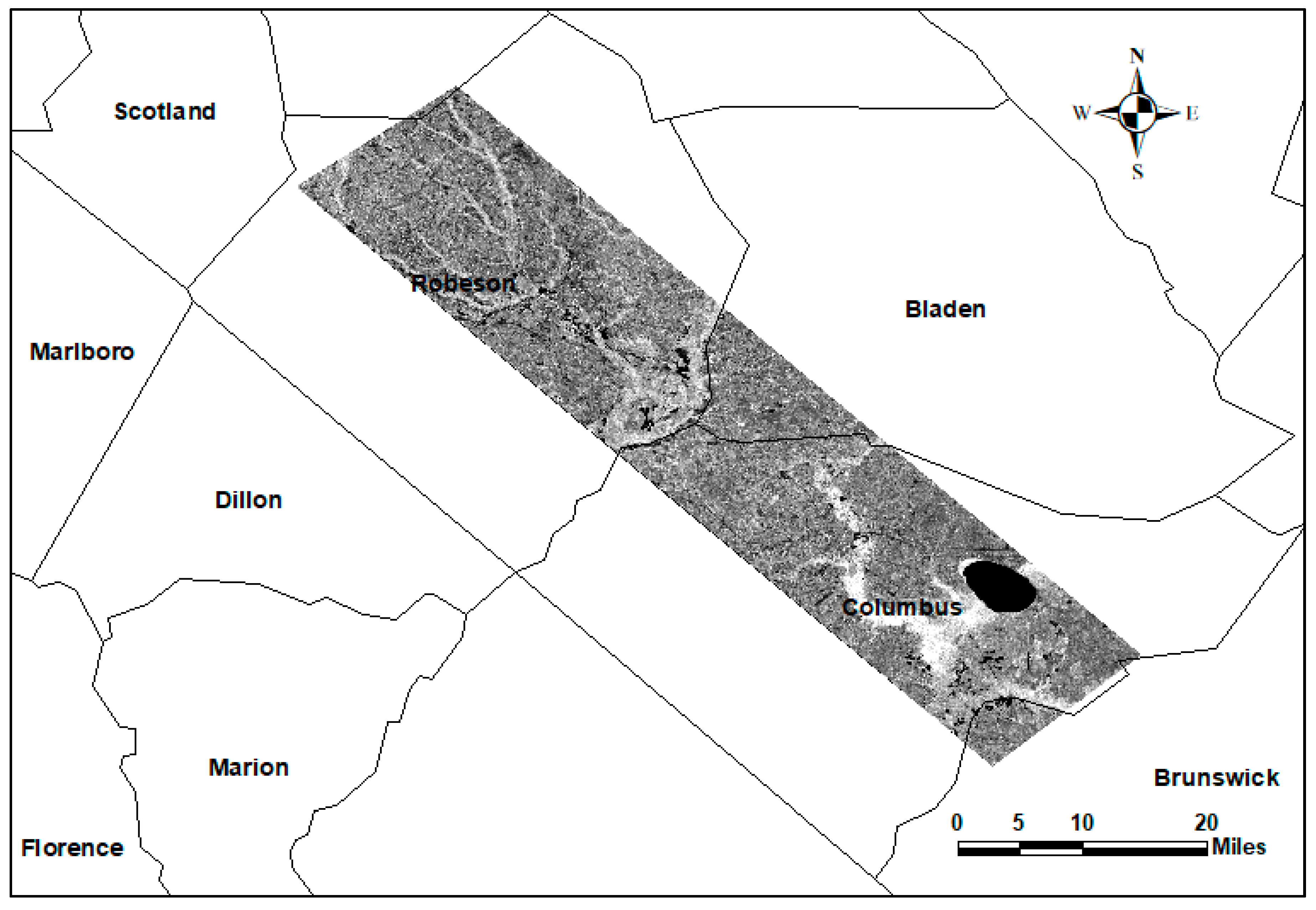
Figure 1. The study area: SAR images of two subareas during Hurricane Florence.
Remotesensing 14 06374 g001
Figure 2. Producer and consumer accuracy for L-band VV polarization.
Remotesensing 14 06374 g002
Figure 3. The accuracy assessment of the UAVSAR L-band VH-polarized data for flood mapping: (a) confusion matrix for training the RF model, (b) producer and consumer accuracy for training, (c) validation error matrix for the classification, and (d) producer and consumer accuracy for validation.
Remotesensing 14 06374 g003
Figure 4. Classification results obtained from the UAVSAR L-band VV (a) and VH (b) polarized data.
Remotesensing 14 06374 g004
Figure 5. The accuracy assessment of the UAVSAR L-band dual-polarized data for flood mapping: (a) confusion matrix for training the RF model, (b) producer and consumer accuracy, and (c) validation error matrix for the classification.
Remotesensing 14 06374 g005
Figure 6. Classification results obtained from the UAVSAR L-band dual-polarized data.
Remotesensing 14 06374 g006
Figure 7. The accuracy assessment of the UAVSAR L-band full-polarized data for flood mapping: (a) confusion matrix for training the RF model, (b) producer and consumer accuracy, and (c) validation error matrix for the classification.
Remotesensing 14 06374 g007
Figure 8. Classification results obtained from the UAVSAR L-band full-polarized data.
Remotesensing 14 06374 g008
Figure 9. The accuracy assessment of the Sentinel C-band VV-polarized data for flood mapping: (a) confusion matrix for training the RF model, (b) producer and consumer accuracy, and (c) validation error matrix for the classification.
Remotesensing 14 06374 g009
Figure 10. The accuracy assessment of the Sentinel C-band VH-polarized data for flood mapping: (a) confusion matrix for training the RF model, (b) producer and consumer accuracy, and (c) validation error matrix for the classification.
Remotesensing 14 06374 g010
Figure 11. Classification results obtained from the Sentinel C-band VV- (a) and VH-polarized (b) data.
Remotesensing 14 06374 g011
Figure 12. The accuracy assessment of the Sentinel C-band dual-polarized data for flood mapping: (a) confusion matrix for training the RF model, (b) producer and consumer accuracy, and (c) validation error matrix for the classification.
Remotesensing 14 06374 g012
Figure 13. Classification results obtained from the Sentinel C-band dual-polarized data.
Remotesensing 14 06374 g013
Figure 14. Floodwater detected by UAVSAR dual-polarized data.
Remotesensing 14 06374 g014
Figure 15. Floodwater detected by S-1b dual-polarized data.
Remotesensing 14 06374 g015
Table 1. Confusion matrix for VV polarization of UAVSAR L-band.
Training Samples (VV)Total
Land Cover ClassGrasslandOpen WaterBare GroundInundated VegetationNon-Inundated Vegetation
Classification ResultsGrassland41846343474
Open water154871515495
Bare ground33427201310
inundated vegetation11015,259815,269
non-inundated vegetation300107688798
Total426556827615,37570122,346
Table 2. Validation error matrix, and producer and consumer accuracy for VV polarization of UAVSAR L-band.
Reference Samples (VV)Total
Land Cover ClassGrasslandOpen WaterBare GroundInundated VegetationNon-Inundated Vegetation
Classification ResultsGrassland404931923152
Open water26186718621919
Bare ground28441937101
inundated vegetation174550191295174
non-inundated vegetation196614970250
Total13019707951862317596
Remotesensing 14 06374 i001
Table 3. The overal accuracy and kappa statistics for the classification results.
PolarizationOA (T)
%
Kappa (T)
%
OA (V)
%
Kappa (V)
%
L-bandVV99.097.8892.3583.65
VH98.596.7691.1380.75
Dual99.6199.1894.9589.13
Full99.4598.9598.6897.47
C-bandVV93.5487.8292.5785.81
VH92.0983.9683.9175.2
Dual97.5394.6191.9682.91
Publisher’s Note: MDPI stays neutral with regard to jurisdictional claims in published maps and institutional affiliations.