Article

Study on Radiative Flux of Road Resolution during Winter Based on Local Weather and Topography

Research Center for Atmospheric Environment, Hankuk University of Foreign Studies, Yongin-si 17035, Gyenggi-do, Republic of Korea
*
Author to whom correspondence should be addressed.
Remote Sens. 2022, 14(24), 6379; https://doi.org/10.3390/rs14246379
Submission received: 6 October 2022 / Revised: 7 December 2022 / Accepted: 9 December 2022 / Published: 16 December 2022
(This article belongs to the Special Issue New Challenges in Solar Radiation, Modeling and Remote Sensing)

Abstract

:
Large-scale traffic accidents caused by black ice on roads have increased rapidly; hence, there is an urgent need to prepare safety measures for their prevention. Here, we used local weather road observations and the linkage between weather prediction and a radiation flux model (LDAPS-SOLWEIG) to calculate prediction information regarding habitual shade areas, sky view factor (SVF), and downward shortwave radiative flux by road direction and lane. Using the LDAPS-SOLWEIG model system, a set of real-time weather prediction data (temperature, humidity, wind speed, and insolation at 1.5 km resolution) was applied, and 5 m resolution radiative flux prediction data, with road resolution blocked by local weather and topography, were calculated. We found that the habitual shaded area can be divided by the direction and lane of the road according to the height and shape of the terrain around the road. The downward shortwave radiation flux data from local meteorological observation data and that calculated from the LDAPS-SOLWEIG model system were compared. When road-freezing occurred on a case day, the RMSE was 20.41 W·m−2, MB was −5.04 W·m−2, and r was 0.78. The calculated information, habitual shaded area, and SVF can highlight road sections vulnerable to winter freezing and can be helpful in the special management of these areas.

Graphical Abstract

1. Introduction

Effects of weather on roads can be largely divided into road driving, traffic flow, and road operation (http://ops.fhwa.dot.gov accessed on 1 October 2020). Major meteorological phenomena, such as rain, snow, and fog, affect road slippage, icing, and driver visibility, thus resulting in road accidents. Furthermore, major traffic accidents are often related to road conditions, vehicle braking, and driving visibility [1,2,3,4,5], severely threatening the lives and safety of people, and are emerging as a national-level social issue. Although the number of road-freezing accidents in winter is small, the death rate associated with such accidents is higher than with other causes [6,7,8,9]. The death rate from traffic accidents due to road icing was four times higher than that in accidents under snow conditions, hence considered a “risk without brakes”; the number of fatalities in the past five years reached 199 [10].
As winter temperatures increased compared to previous years, large-scale traffic accidents caused by black ice on roads have rapidly increased; thus, preparation of safety measures to prevent such accidents is an urgent requirement. Black ice is a thin sheet of ice that occurs locally on roads and is difficult to distinguish with the naked eye; it is most likely to occur on the surface of a road that has been moistened by rain, snow, and fog, or in the early morning or at dawn on a humid day due to a drop in temperature.
Black ice is generated by the interaction of various factors: meteorological factors including local temperature, relative humidity, and precipitation in the road area; environmental factors including altitude, latitude, surrounding topography, and shadow effects; physical factors including shaded areas with little exposure to insolation which are vulnerable to black ice, and areas of roads that are continuously shaded have a similar level of risk as bridge areas [11,12].
The main factors affecting black ice are road surface temperature and pavement condition. Road surface temperature is affected not only by synoptic weather conditions but also by the length of the tunnel, road material (i.e., asphalt, concrete), and road location. In addition, road surface temperature is a factor directly involved in black ice and a parameter that determines the road surface condition.
Among road surface conditions, black ice may or may not be accompanied by precipitation. Black ice accompanied by precipitation is formed when rain at freezing temperatures meets a cold road surface, and the precipitation at this time is called freezing rain [13,14,15]. In the absence of precipitation, black ice is generated when water vapor in the atmosphere condenses on a cold road surface which causes a further decrease in temperature due to radiative cooling [16]. Therefore, road surface temperature is a vital factor in determining black ice [17]. In general, black ice accompanied by precipitation can be forecast based on synoptic weather in a relatively wide area, but black ice without precipitation is difficult to forecast as it occurs locally.
There are cases where road weather forecast models related to road icing in winter were developed using not only synoptic weather information but also observation data from road meteorological stations and radar precipitation measurements. These models generate not only road surface temperature but also a road surface condition classification and driving condition index [18]. However, despite the development of the Road Weather Information System (RWIS), the current road surface temperature prediction model has limited performance at the resolution that reproduces complex real environments [19].
Research on black ice in Korea was mainly conducted through observations in areas vulnerable to black ice [20,21,22,23,24,25]. Kim et al. [10] collected meteorological and road surface condition data with a mobile meteorological observation vehicle and suggested the following conditions as favorable for road icing. On bridges, where cold winds blow freely, at tunnel entrances, in clear weather and weak winds, and in valleys or valleys adjacent to mountainous areas where cold pools form easily due to radiative cooling, ice is well maintained by the shade effect of vegetation after rain or snow. Shaded areas, where ice does not melt quickly, were suggested as favorable conditions for road icing. The authors in [25] prepared a road thermal map with a mobile meteorological observation vehicle and comparatively evaluated the spatiotemporal synthesis method for creating a thermal map.
Although fixed and mobile observation systems have been established to observe road weather and surface conditions, there is still a limit to predicting the risk of black ice [26]. Field application remains difficult because of the lack of spatially detailed meteorological fields corresponding to the road area and sufficiently detailed road surface temperature or condition data [27].
In order to supplement the spatial resolution of stationary point-based observation data, research on predicting black ice using a physical or statistical model with mobile road section-based observation data is also being conducted [12,22,28]. Previous studies on the occurrence of black ice, using weather and road parameters, reported that “shadow effect and change in relative humidity” should be considered for road conditions in Korea, which are characterized by local climate variability and topographical complexity.
Road surface temperature can vary substantially on a given road. This is dependent on the surrounding topography and other common characteristics, where there are obstacles such as cutouts on both sides of the road; in such cases, a shadow is formed on the road surface, and less solar radiation energy reaches the road surface. Consequently, the usable energy on the road surface is also reduced, resulting in a lowered road surface temperature. In addition, canyon-shaped terrain causes stronger winds compared to the surrounding areas; moreover, in the presence of moisture inflow when the road surface temperature is lower than the surrounding conditions, the possibility of black ice formation increases [25].
Here, we focus on the shadow effect, an important factor in the occurrence of black ice as revealed by observations in the absence of precipitation and the blocking of the downward shortwave radiation flux and emission of upward longwave radiation. The utility of the winter solar radiation model is presented by using detailed road weather field data, the direction and shape of the road, and a detailed structure of the surrounding area. In addition, using the solar radiation model (i.e., SOLWEIG, Solar, and Longwave Environmental Irradiance Geometry), combined with local weather forecasting data (i.e., LDAPS, Local Data Assimilation, and Prediction System) of the road under study, a real-time downward and upward shortwave and longwave radiative flux prediction model with road resolution was developed and implemented. Among them, the downward shortwave radiant flux was compared with ground observation data, and the upward longwave radiant flux was compared with the satellite image data.

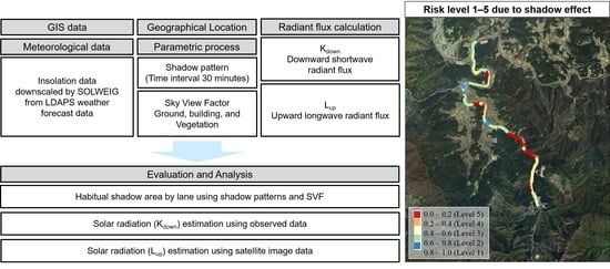
2. Materials and Methods

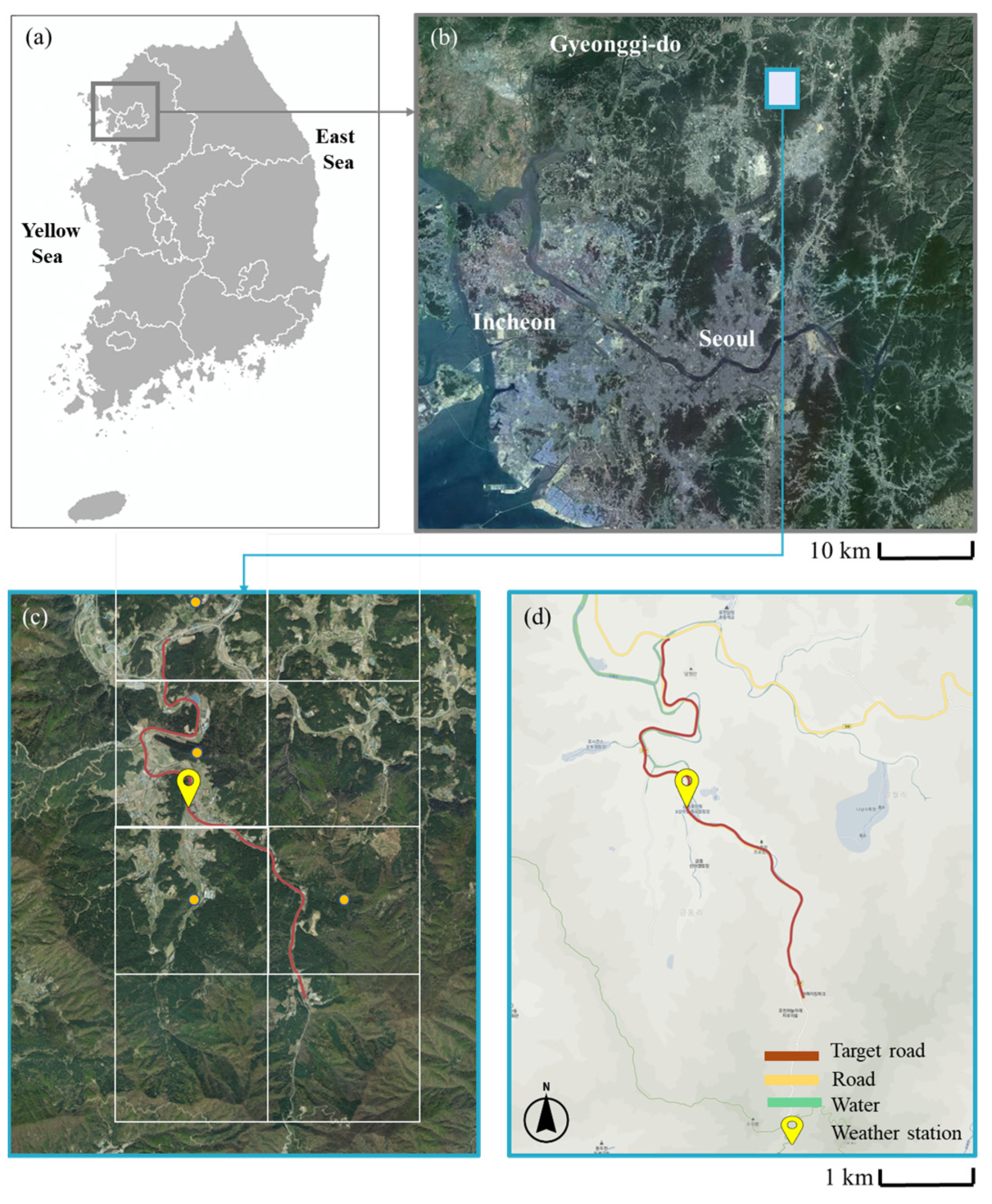
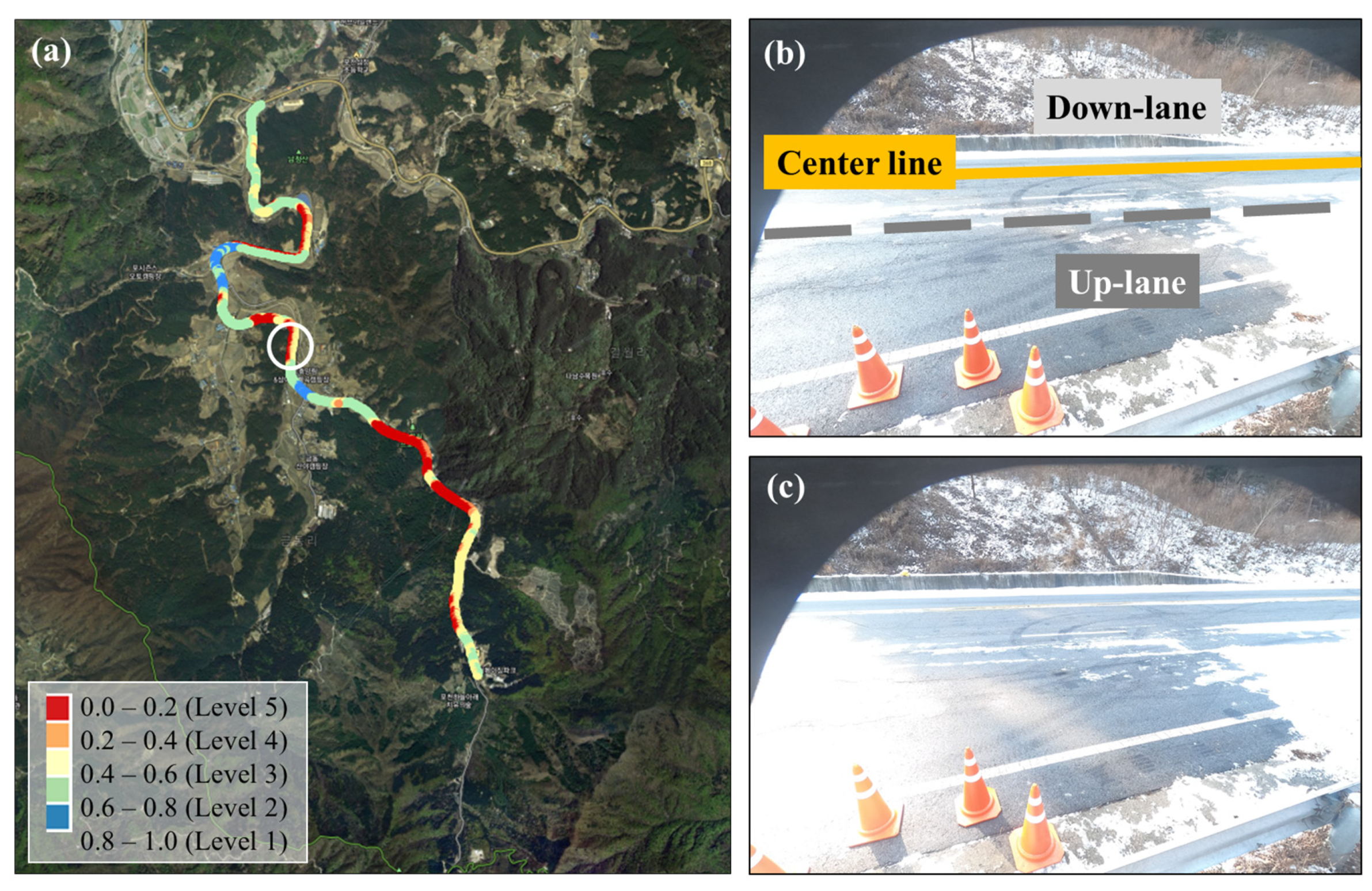
2.1. Study Area and Analysis Dates

The Pocheon regional route 379 located in the northern part of South Korea, a 6 km two-lane road with a mean elevation of 256.78 m, was analyzed here. A 5 × 6 km area incorporating the road was selected for the radiation model (Figure 1c), as it contains mountainous terrain in the E–W and N–S directions, and lower temperatures are maintained at higher elevations compared with other areas. Figure 1a shows that the study area is the northern region of South Korea, and Figure 1b shows the surrounding environment of Figure 1c, which is a model simulation area. Figure 1c,d show that the road to be analyzed is narrow and surrounded by high mountains. The white square in Figure 1c is the grid representing the spatial resolution of the meteorological prediction model, and the meteorological prediction data of the grid with yellow round marks were used as input data.
Days with freezing risks were determined by inputting the measured air, dew point, and road surface temperatures, as well as the relative humidity, during the observation period (January–April 2021) into the road-freezing evaluation algorithm proposed by [23] (Figure 2). This was performed to identify days with high ratios of “road-freezing conditions” and “freezing is highly probable” scenarios. The freezing determination algorithm uses weather factors to ultimately determine six types of conditions: “dry condition”, “freezing highly probable”, “no road-freezing”, “road-freezing condition”, “road-wet condition”, and “unsuitable road-wet condition”.
Using the data during the observation period (from 26 January to 32 March 2021, see Section 2.5), the road-freezing prediction results were calculated with this algorithm. The result was evaluated via a confusion matrix with observation data [29] (Figure 3). A total of 18,720 data collected as observational data (observed at 5 min intervals for 65 days) were sorted into 18,215 after applying an algorithm to remove omissions and outliers.
The true positive (TP) value in which both prediction and actuality were frozen was 4488, and the true negative (TN) value in which both prediction and actuality were non-freezing was 11,698. The false positive (FP) value, which was predicted to be frozen but was actually non-freezing, was 1533, and the false negative (FN) value, which was predicted to be non-freezing but was actually frozen, was 496. Accuracy was 0.8886, precision was 0.7453, and sensitivity was 0.9004.
Using this algorithm with such accuracy, 4 days with high freezing ratios were selected for further analysis (Figure 2): 24 January (62.6%), 25 January (56.8%), 10 February (57.4%), and 11 February (56.8%). Hourly air, dew point, and road surface temperatures, which have the largest influences on the evaluation algorithm, were retrieved for the selected days. Freezing conditions occurred before sunrise and after sunset on all 4 days when the road surface temperature was lower than that of the surrounding air (Figure 4).

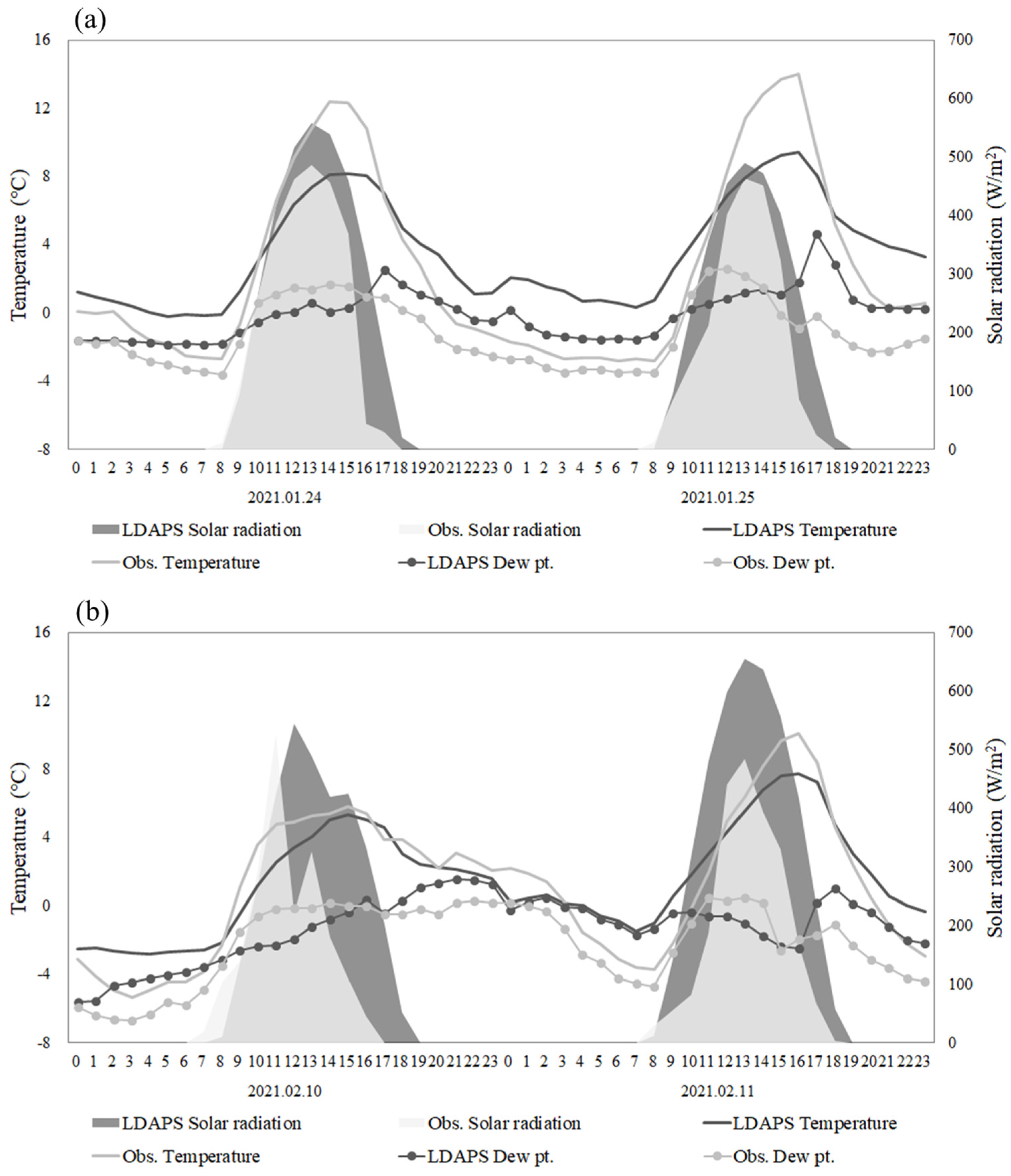
2.2. LDAPS Weather Prediction Data

The Local Data Assimilation and Prediction System (LDAPS), operated by the Korean Meteorological Administration, has a spatial resolution of 1.5 km and a 70-layer vertical resolution of up to 40 km. The system receives boundary fields at 3 h intervals from the Global Data Assimilation and Prediction System (GDAPS): at 00, 06, 12, and 18 UTC for 36 h predictions and at 03, 09, 15, and 21 UTC for 3 h predictions [30]. Here, the meteorological prediction field data of the research area were constructed, which could be applied to the radiative flux–road surface temperature–road-freezing prediction system. Only the LDAPS point data corresponding to the SOLWEIG simulation results (direct and scattered total solar radiation fluxes, temperature, dew point temperature, and wind components) were extracted, and mean values were calculated for the model input (Figure 1c).
Four grid points were included in the 1.5 km resolution LDAPS data in the 5 × 6 km research area, and the hourly meteorological input data of the SOLWEIG model were constructed by averaging the three grid meteorological data. Figure 5 shows the central point of the grid corresponding to the research area as a point. The LDAPS-derived temperature, dew point, and radiation flux data were compared with the meteorological station data for the four selected days (Figure 5), during which the observed diurnal temperature variations were much stronger than those predicted. In particular, the observed temperature at 1300 LST on January 25 was ≤3.5 °C warmer than the LDAPS value. A similar trend was observed for the dew point, with the maximum discrepancy observed during the early afternoon of 25 January. The LDAPS-predicted solar radiation values were slightly higher on 24–25 January but exhibited similar diurnal patterns. Notably, the maximum solar radiation differences were observed on February 11, when similar patterns were offset by a large time-lag. As the measured values were location-specific (one-point measurements), the land cover and terrain types of the adjacent areas had strong influences, whereas the LDAPS-predicted values corresponded to the means of the 1.5 km resolution grids in the study area. Since LDAPS has a resolution of 1.5 km, it does not seem to reflect the complex terrain and road characteristics of the road area to be analyzed in detail. The solar radiation, reduced by the surrounding terrain elevation and road type, could not be simulated. Thus, the solar radiation was higher than the observed solar radiation.

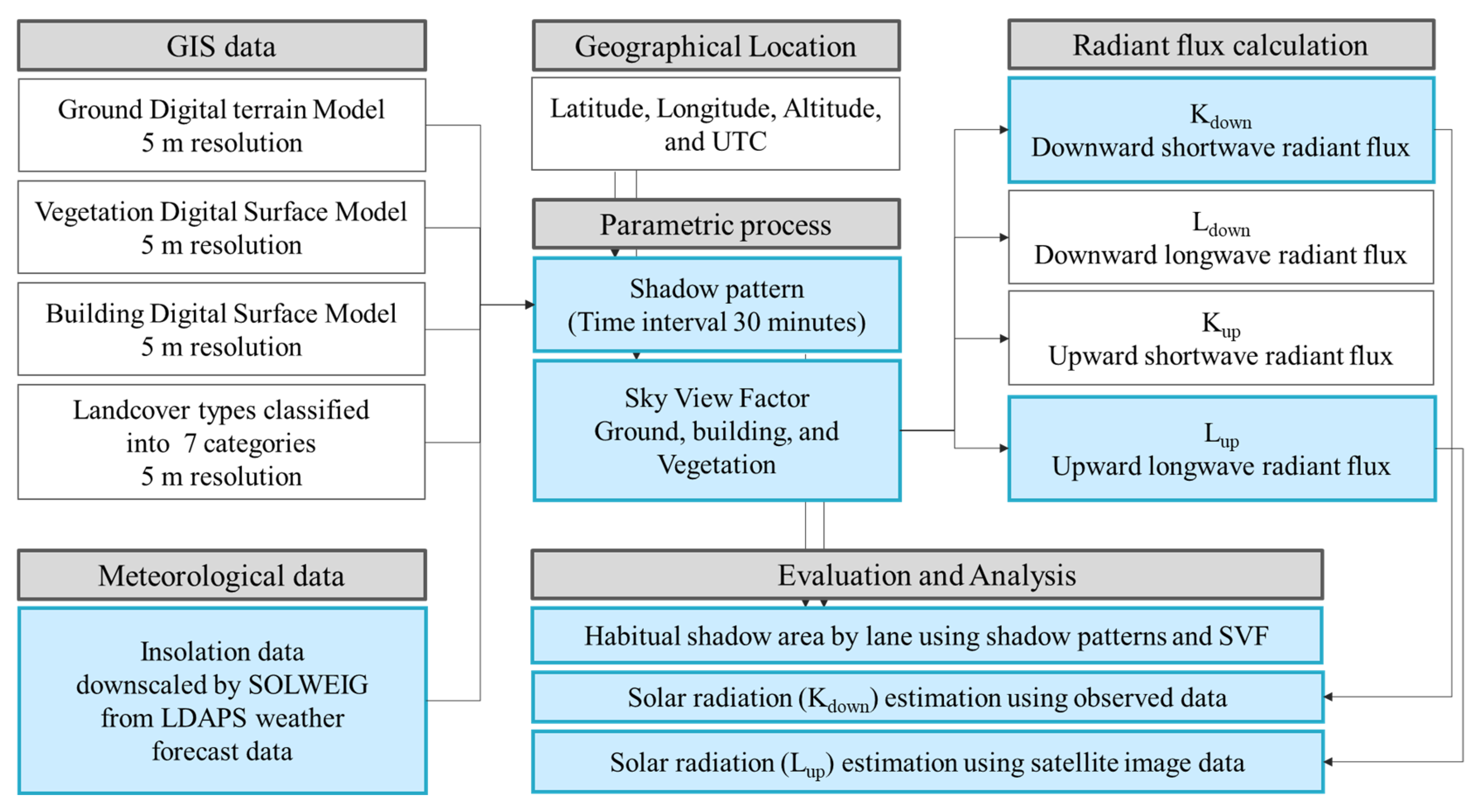
2.3. SOLWEIG Solar Radiation Model

The SOLWEIG model used in this study (ver. 2015a) is a high-resolution solar radiation model developed by the Göteborg Urban Climate Group of the University of Gothenburg, Sweden [31]. The model calculates mean radiant temperatures (Tmrt) from 3D radiant fluxes using urban physical features, including building or vegetation heights [32]. From this model, it is possible to calculate the shadow pattern at 30 min intervals according to the solar altitude of the target area and to calculate the sky view factor (SVF) for each grid considering the topography, building, and vegetation height. Previous studies evaluating the calculated radiation using the SOLWEIG model aimed to suggest human thermal comfort through building design, form, or structure [31,32].
Ref. [33] confirmed the SOLWEIG model’s ability to simulate radiation fluxes, and [34] demonstrated a successful model performance for sunny and cloudy summer and winter days in the high-density building area of Seoul, achieving R2 and root mean square error (RMSE) values of 0.98 and 25.84 W·m−2, respectively, for upward longwave radiation (Lup). Additionally, [35] used SOLWEIG to refine the downward shortwave radiation flux and upward longwave radiation flux and analyzed the relationship between the shaded area and the road surface temperature. The accuracy of observation data was evaluated by simulating the downward shortwave radiation flux by the three-dimensional structure of urban buildings and vegetation and by simulating the upward longwave radiation flux by land cover condition [36].
Here, a digital surface model (DSM) with 5 m resolution and land cover data for the winter of 2021 were used as ground boundary data for the SOLWEIG model for the research road area. In addition, as the initial meteorological data, LDAPS meteorological prediction data (i.e., temperature, humidity, wind speed, and radiation) were input to simulate the shortwave and longwave radiation flux of the region, downward and upward.

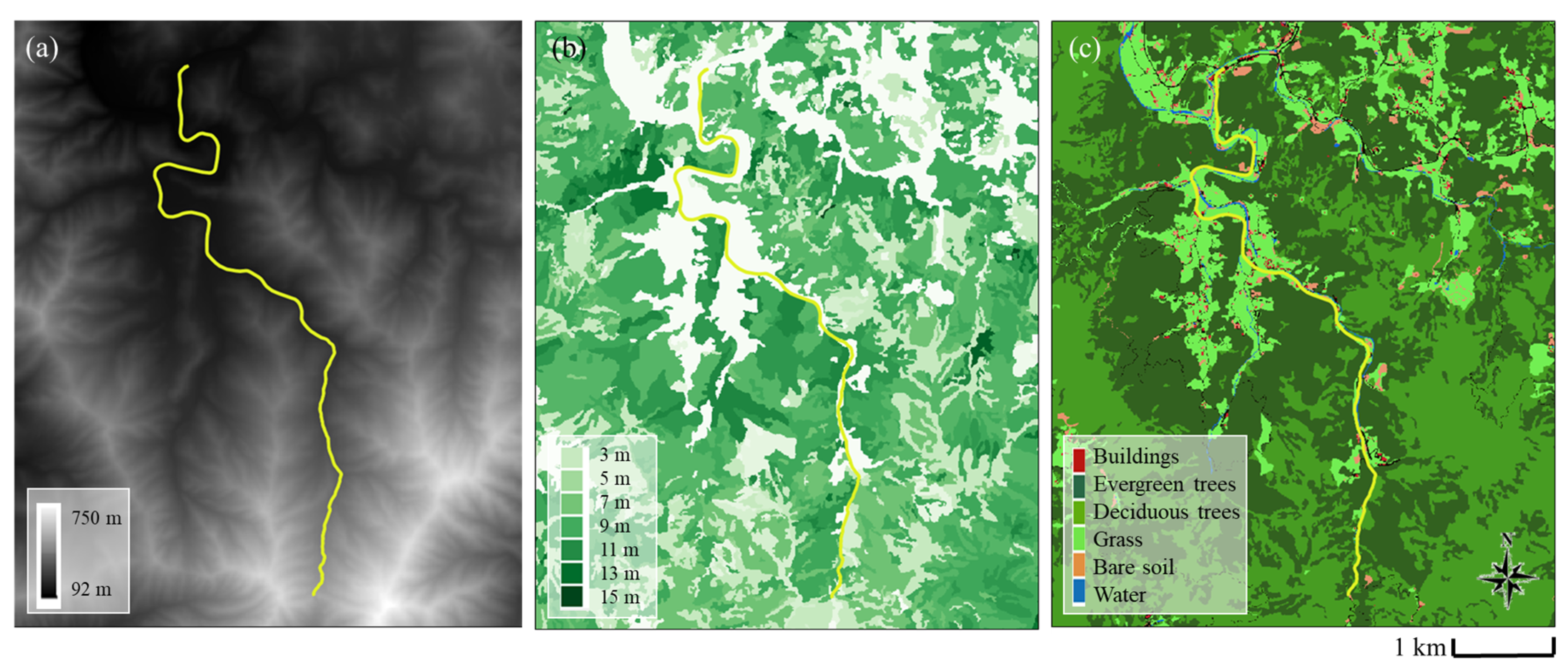
2.4. GIS Data of Road Resolution

To construct high-resolution road-level data, a numerical contour map was obtained from the National Geographic Information Institute at the National Spatial Data Infrastructure (NSDI) portal [37] and used with road name, location, and width data obtained from the road transport logistics directory of the Ministry of Public Administration and Security. In addition, a SOLWEIG land cover database was created by reclassifying land cover data (1 m resolution) obtained from the Environmental Geospatial Information Service [38] and a canopy digital surface model (CDSM) using a forest type map (1:5000) obtained from the Korean Forest Service. To construct the ground and building DSM, the road name, building address, and number of floors were acquired from the Ministry of Public Administration and Security. The building heights were calculated as 3.5 m·floor−1 and added to the ground elevation to calculate the DSM (Figure 6). Each dataset was scaled to 5 × 5 m resolution using QGIS (v.3.16.2). QGIS is a user-friendly open-source Geographic Information System (GIS) licensed under the GNU General Public License. QGIS is an official project of the Open-Source Geospatial Foundation (OSGeo). The ground and building DSM elevations in the study area ranged from 92–751 m, and the vegetation CDSM was ≤15 m, with deciduous and evergreen forests comprising the predominant land cover types. Seven land cover types were identified, and different parameters (e.g., albedo and emissivity) were recorded for each type (Table 1).

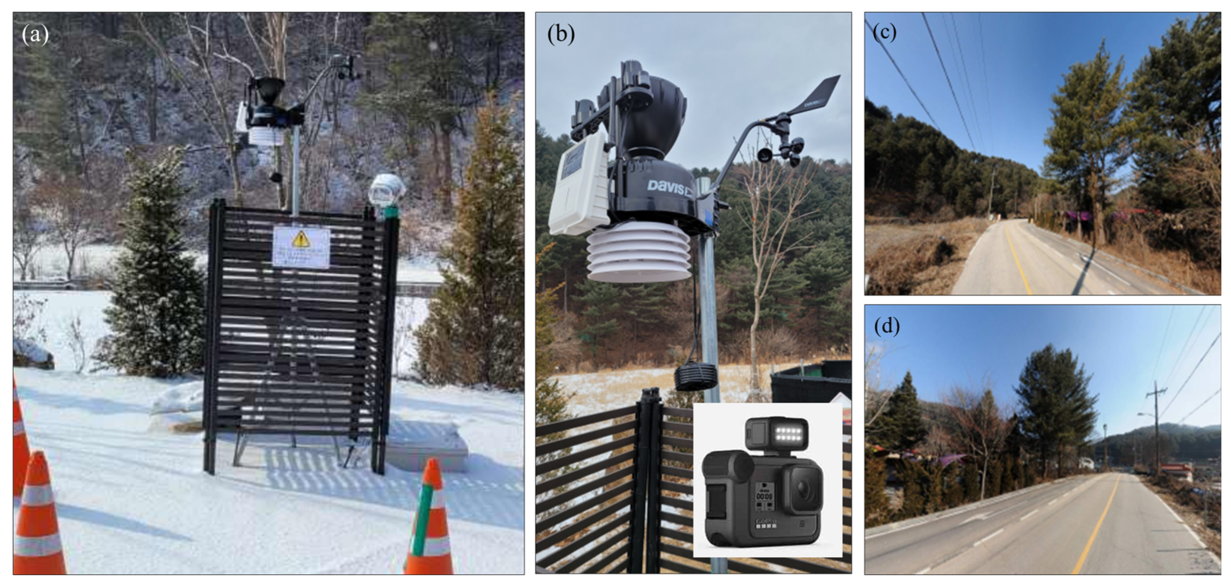
2.5. Observation for Radiation Verification

Previous studies that have evaluated radiation, calculated using the SOLWEIG model, aimed to make suggestions for human thermal comfort through building design, morphology, or structure [32,33]. However, in this study, because the effect of road cover (asphalt) must be considered to evaluate the road-freezing risk [39], a measurement system was installed for model validation.
The meteorological observation equipment was DAVIS’ Vantage Pro2 Plus (Davis Instruments, Hayward, CA, USA), and the road surface temperature was DAVIS’ embedded temperature sensor. Road footage was captured with a micro-miniature camera to monitor the road-freezing conditions, and a GoPro HERO8 model was used in consideration of the time-lapse function and night photography (Figure 7 and Table 2).
As the surface temperature is markedly affected by the type of ground material on the surface [40], the measurement system was installed at close proximity to the road.
A meteorological observation station was placed along the test road to evaluate the radiation flux and observe the road surface and dew point temperatures. A composite slope was considered when selecting the location of the station, drawing on composite slopes of 2–3% and ≥7% that are most vulnerable to traffic accidents. Composite slope considers the cross and longitudinal slopes simultaneously in the curved part of the road and is expressed as a composite slope value of both cross and longitudinal slopes.
Accordingly, a location was selected that contained overshadowed areas (shadow pattern, as calculated by SOLWEIG), the appropriate composite grades, and ease of installation (near buildings). The selected location (37.944774°N, 127.126552°E) was 3.3 km from the starting point at the northern end of the road. From 26 January to 31 March 2021, air, dew point, road surface temperature, RH, wind speed and direction, atmospheric pressure, precipitation, and solar radiation were recorded every 5 min, while road surface conditions were simultaneously captured by a camera (Figure 7). Data were wirelessly transmitted from the solar-powered station to a data logger and monitored remotely. Road photographs were used to compare the algorithm and ground conditions, and the observed radiation fluxes were used to verify the SOLWEIG model results. The overall flowchart of this study is shown in Figure 8 and is divided into data construction, model connection, result calculation, and evaluation.

3. Results and Discussion

3.1. Shadow Pattern Analysis by Road Lane

Shadow pattern values were calculated at 30 min intervals on 21 January 2021 using GIS input data, latitude, longitude, elevation/height, and UTC time. The lower the calculated value, the more the grid is affected by shadows (lower downward shortwave radiation flux). No shadow effect (with downward shortwave radiation flux) is represented by one. Since the longer the shadows are formed, the less they are affected by downward shortwave radiation, the values for the presence or absence of shadows calculated with a 5 m resolution grid were divided into five categories and analyzed. The value that produces the most shadows (the amount of downward shortwave radiation flux is very small), 0~0.2, is classified as Level 5, 0.2~0.4 is Level 4, 0.4~0.6 is Level 3, 0.6~0.8 is Level 2, and 0.8~1.0 is Level 1. Since the area most affected by the shadow is the habitual shade area, the road surface temperature is the lowest and the risk of freezing is high, so Level 5 is the highest level. The potential risk due to shadows was divided into five stages, and the risk distribution was analyzed along the road according to the daily average shadow presence or absence value.
Risk levels 1–5 accounted for 7.11%, 36.78%, 23.62%, 7.34%, and 25.14% of the day, respectively. The shadow patterns were analyzed according to the 5 m resolution map and were divided into up-lane (northbound) and down-lane (southbound). At this scale, the risk distribution profile changed: Level 2 remained the most frequent up-lane risk level (40.41%), while Level 5 was the most frequent down-lane risk level (36.85%; with an up- to down-lane ratio of ~1:3), implying that shadow effects dramatically affected the down-lane. Accordingly, the areas that fell under Level 5 were located in overshadowed areas and were analyzed further. Table 3 lists the 30 min shadow patterns divided into up- and down-lane values, as well as the Level 1 and 5 ratios for each time, where the lower the shadow pattern value, the higher the shadow effect. According to the direction, the road was divided into up- and down- lanes, and the ratios of Levels 1 and 5 were presented. If there was a shadow (no downward shortwave radiation), it was classified as Level 5, and if there was no shadow (downward shortwave radiation present), it was classified as Level 1. When looking only at the ratios of Levels 1 and 5 across the entire road, it can be quantitatively confirmed that the ratio of Level 5, which is heavily affected by shadows, varies over time. The shadow pattern value of the down-lane was lower than that of the up-lane during the daytime; in particular, large differences were observed in the photos captured at 5 min intervals from 11:00 to 14:00 (Figure 9a). Figure 9b,c are the photos at 12:09 and 12:39, and the presence or absence of shadows was observed at intervals of 30 min. Each lane exhibited differences in shadow patterns during the daytime, as the shadow length is inversely proportional to the sun’s altitude. Thus, we concluded that the daytime down-lane was more dramatically affected, given that the southward lane was more frequently overshadowed by the surrounding topographic features and vegetation.

3.2. Sky View Factor Analysis

SVF is a critical factor that quantifies the effects of obstacles obscuring the sky view, thereby helping to explain complex urban geometry and the relationship between incident and scattering radiation fluxes. Longwave radiation provides evidence of the moderating effects of surface geometry on the magnitude of physical cooling emitted by the Earth’s surface. The authors in [40] demonstrated that SVF is one of the factors determining road surface temperature variability, as well as the occurrence of shadow patterns and their duration. SVF values are indexed on a scale from zero (fully obscured by the surrounding terrain, buildings, and vegetation) to one (completely free of obstacles and on flat ground). In this study, SVF was calculated using the method described by [32]. The SOLWEIG model produces two types of SVF: buildings (and ground) and vegetation, where the former is further broken down into the cardinal directions (north, south, east, and west) and the total. Low SVF values are observed primarily in mountainous areas with high altitudes, whereas high SVF values commonly occur in flat terrain at low altitudes. Incoming solar radiation levels in both types of areas are less affected by the surrounding land cover and terrain morphology compared to the adjacent areas. To determine the differences between the lane shadows and SVF values, shadow patterns, SVFbuilding-ground and SVFvegetation values were analyzed for each risk level in the overshadowed areas, where higher levels indicate lower SVF values under the influence of built-up, topographic, and vegetation features. This is because, even at the same level, the roads heavily affected by shadows may appear differently depending on the ascending and descending lines, and the shadow pattern value shows this numerically, enabling quantitative comparative analysis. In addition, by comparing the SVF values of the two types together, it is possible to quantify the factors and degree of influence that affect the shadow of the road among the topography and vegetation (Table 4).
The shadow pattern values of the up- and down-lanes were similar in Levels 1–3, but Levels 4 and 5 had larger values in the down-lane, indicative of greater shadow effects. For Levels 4 and 5, the overshadowed areas were affected more by vegetation than by buildings or ground topography. In particular, the Level 5 difference in SVFvegetation between the up- and down-lanes was more than double, demonstrating the strong shadow effect of the nearby vegetation. This pattern is largely attributable to the geomorphological characteristics of the road, coupled with the numerous densely vegetated areas immediately adjacent to the down-lane. As Korea is a right-hand-traffic country, we numerically confirmed that tall vegetation on the right-hand side of the driving lane increased the shadow effects in the nearest lane (down-lane).

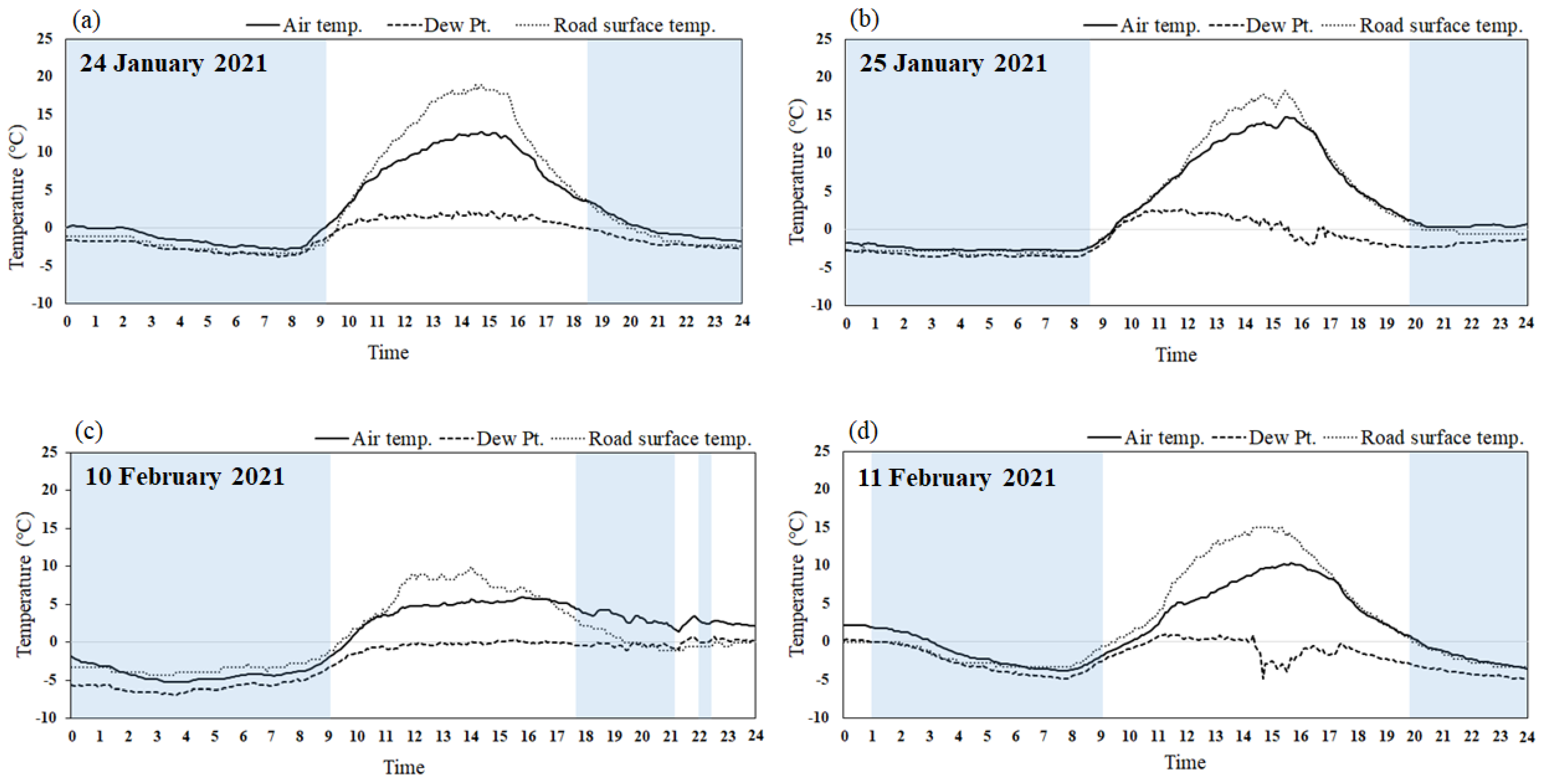
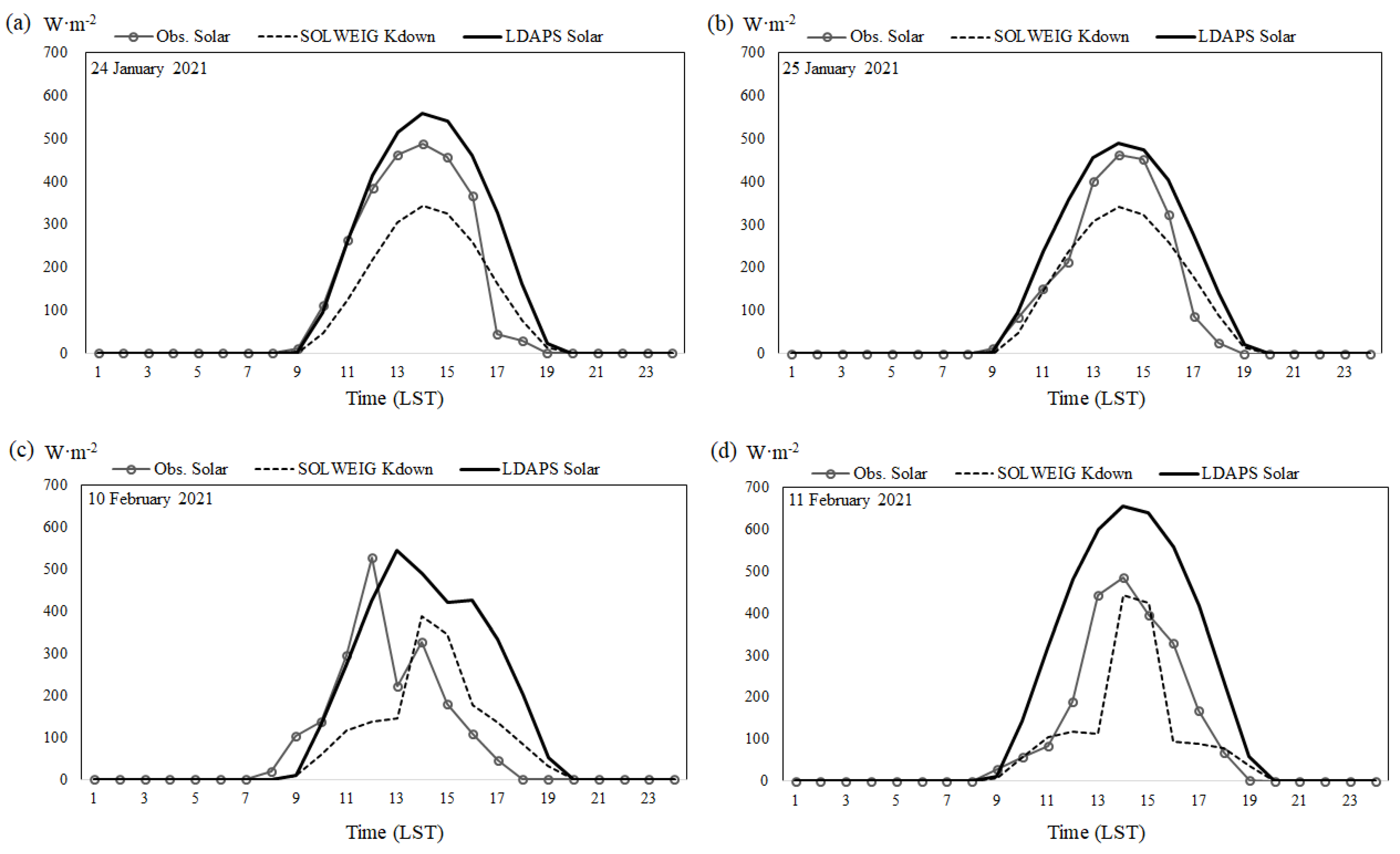
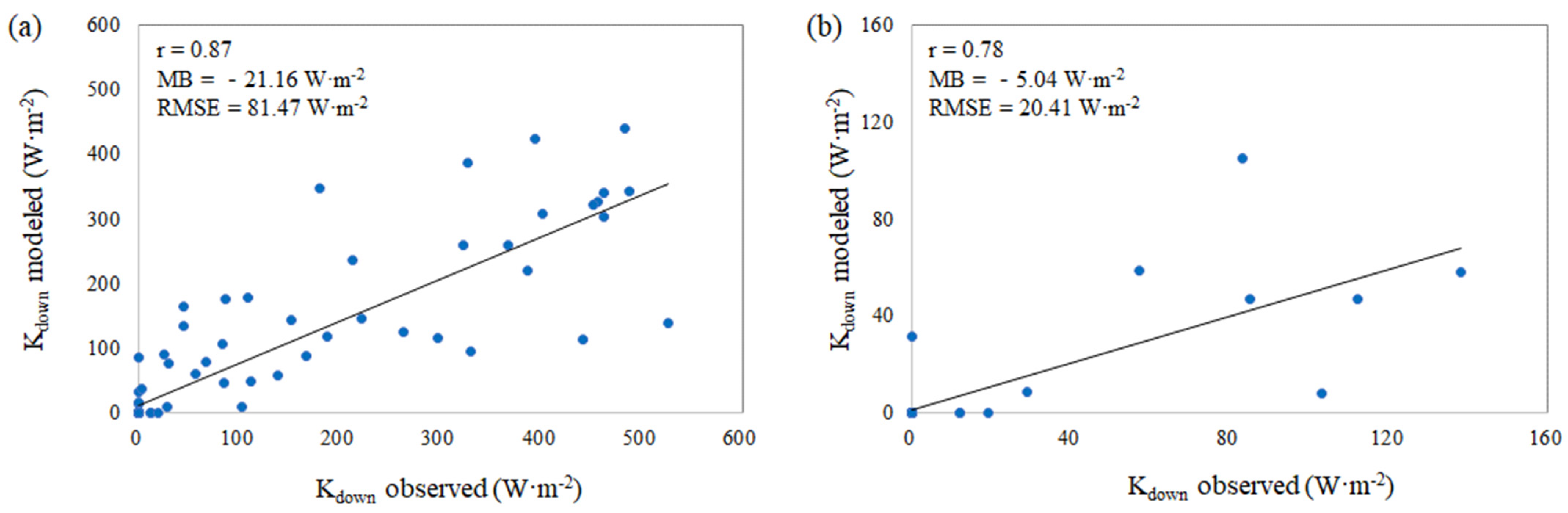
3.3. Downward Shortwave Radiation Evaluation Using Observed Data

To evaluate the downward shortwave radiation fluxes calculated by the SOLWEIG model, the Kdown (downward shortwave radiation) values for the grid corresponding to the location of the meteorological station were extracted and compared with the observations. The observations were also compared with the LDAPS-prediction radiation fluxes to assess the accuracy of the SOLWEIG output and initial radiation input values. The SOLWEIG radiation values were the lowest, whereas the LDAPS were the highest. In Figure 10a,b, the observed Kdown fluxes showed a distribution similar to the radiative flux of LDAPS, while Figure 10c,d show a similar distribution to the detailed radiative flux. A correlation analysis was performed to verify the model. The correlation coefficient (r) indicates the strength of the relationship between the estimated and observed values [–1, 1], where 0 indicates no linear relationship between the two variables. The mean bias (MB) is the mean difference between the modeled and observed values and indicates the tendency of a value to under- or overestimate the observations. An MB of 0 indicates that no error is present [39]. The RMSE measures the overall prediction accuracy of the derived trend line and thus scales with the differences between the estimated and true values.
The data for each selected day and the estimated times of the freezing road conditions were extracted and divided into two categories. The RMSE of all four selected days was 81.47 W·m−2, and the MB was −21.16 W·m−2, which indicate an underestimation of the modeled values (Figure 11a). For the estimated times of freezing conditions, the MB (−5.04 W·m−2) also indicated an underestimation of the modeled values, with a similar RMSE of 20.41 W·m−2 (Figure 11b). The correlation coefficient (r) was 0.87 for the four selected days and 0.78 during the estimated road-freezing times, indicating a relatively strong degree of correlation.

3.4. Upward Longwave Radiation Evaluation Using Satellite Imagery Data

To verify the modeled radiation flux distributions calculated via the SOLWEIG, upward longwave radiation (Lup), satellite imagery was compared using Landsat-8 (L8 OLI/TIRS C2 L1) thermal infrared images. Data corresponding to the atmospheric window between 10 and 12 μm were selected (Band 10, 11 μm; 30 m × 30 m resolution). Images taken on 24 December 2020 and 26 February 2021 corresponded most closely to the selected study dates and had <20% cloud cover (Figure 12).
To determine the surface temperatures, spectral radiance was calculated using the linear regression constant corresponding to Band 10, as well as the brightness temperature from Landsat-8, using the calculated spectral radiance and correction factors (K1 and K2). To calculate the surface temperature at a 30 m resolution, the emissivity for each land cover type was applied to the calculated brightness temperatures. As a 30 m resolution is insufficient to discern the precise location of a two-lane regional road, the road coordinates were marked on the retrieved images.
As the satellite images were acquired near 1100 LST, they were compared with the distribution profile of the average daytime Lup. The images from 24 December 2020 were compared with the results for 24 January 2021, and the images from 26 February 2021 were compared with the results for 11 February 2021. The surface temperatures were calculated from the upward longwave radiation according to the following:
T o = ( L i j ε g σ ) 4
where σ is the Stefan–Boltzmann constant (5.67 × 10⁻⁸ kg·s−3·K−4), and εg is the emissivity of the ground (0.95).
The surface temperatures calculated from the satellite imagery for these two dates ranged from −0.36 to 4.76 °C (a) and from 6.34 to 13.14 °C (c), respectively; whereas the surface temperatures modeled using Lup radiation in the SOLWEIG model ranged from 5.07 to 8.46 °C and from 3.53 to 7.15 °C, respectively, indicating a much narrower temperature range (Figure 12). The scatter plots between the two surface temperatures indicate that the imagery from 24 December 2020 and the SOLWEIG results for 24 January 2021 yielded a correlation coefficient (r) of 0.32 and an RMSE of 4.27 °C, whereas the February imagery and SOLWEIG results yielded a correlation coefficient (r) of 0.37 and RMSE of 4.54 °C (Figure 13). In previous studies, evaluations using meteorological observations of roads were conducted using a point-based method [23,32] or mobile observations using a car [41,42]. However, in this study, the spatial distribution was evaluated to determine the overall simulation accuracy in the study area. In particular, because the downward shortwave radiation is affected by topography [43], evaluation of the spatial distribution of radiation fluxes calculated in consideration of the detailed topography is required. Both selected days exhibited positive correlations, and the narrower modeled temperature ranges may be attributable to the difference in the image resolution when converting from a 5 m to 30 m resolution.

4. Conclusions

In order to better deal with dangerous black ice accidents in winter, we utilized scientific information for a fundamental solution. Through local weather observations of the road in the study area and the linkage between the weather prediction and radiation flux model (LDAPS-SOLWEIG), prediction information about the habitual shade area, SVF, and downward shortwave radiative flux by road direction and lane was calculated.
Using the LDAPS-SOLWEIG model system, a set of real-time weather prediction data (temperature, humidity, wind speed, and insolation at 1.5 km resolution) was applied, and 5 m resolution radiative flux prediction data with road resolution blocked by local weather and topography were calculated. According to the effect of applying the high-resolution surface boundary data, it was confirmed that the habitual shaded area was divided by the direction and lane of the road according to the height and shape of the terrain around the road and that the downward shortwave radiation flux was detailed over time.
The downward shortwave radiation flux data from local meteorological observation data were compared with that calculated from the LDAPS-SOLWEIG model system. For all dates selected as case days, the RMSE was 81.47 W·m−2, MB was –21.16 W·m−2, and the correlation coefficient (r) was 0.87. For the time when road-freezing occurred within the case day, the RMSE was 20.41 W·m−2, MB was −5.04 W·m−2, and r was 0.78. For the time when road-freezing occurred, the error of the value of the downward shortwave radiation flux simulated by the model was smaller. Surface temperature verification was also conducted based on comparisons of Lup values and those obtained from Landsat satellite imagery, confirming a positive correlation between the two analyzed dates and the corresponding images. However, the effects of the different spatial resolutions between SOLWEIG (5 m, high resolution) and Landsat imagery (30 m, medium resolution) cannot be ruled out. More accurate verifications of spatial temperature distributions will require datasets from multiple observation stations and higher-resolution satellite imagery.
The downward shortwave radiation flux decreased in the vicinity of the road due to vegetation, buildings, habitual shaded areas due to topographical characteristics, and blocking of the sky view. These results were mainly pertaining to the right side of the driving lane, and as the right lane rule is followed in Korea, the potential risk of road icing may increase due to the influence of the topographical features on the right side.
In previous studies, local weather, road environment, and surrounding terrain were suggested as factors that can affect road surface temperature, and the LDAPS-SOLWEIG model system can solve these factors with the resolution of road resolution. It can be applied not only to a wide road area but also to a relatively narrow road section, and it was possible to implement a spatial prediction model in the form of a map rather than a point-based model.
In addition, even without fixed and mobile meteorological observations, this model system, which reflects high-resolution GIS data, made it possible to predict the road surface temperature, which may render the road vulnerable to road-freezing. This study evaluated the detail and accuracy of the downward shortwave radiation flux. With the results of the accuracy evaluation of the upward longwave radiation flux, as presented by [44], it is now possible to calculate the net shortwave and longwave radiation flux with higher accuracy.
However, to further secure the scalability and accuracy of the model, the reliability of the observation data is important, and the accuracy of the standard specification of the used observation sensor, the year and standard of installation, and the sensitivity of the sensor should be verified.
In this study, direct verification was limited due to the absence of a longwave radiation sensor installed on the road in the study area. Shortwave and longwave radiation sensors are installed on the “Smart Highway Demonstration Road” in Korea. Thus, it is expected that the model’s expansion and accuracy can be improved using the data in the future.
This model system can be used to predict potential road-freezing vulnerable sections, and the prediction time can calculate detailed radiation flux prediction data for up to 36 to 60 h, which is the prediction time of LDAPS. In addition, the calculated information, habitual shaded area, and SVF can list road sections that are vulnerable to road-freezing and can be helpful in special management of areas with risk of freezing in winter, such as securing a budget for snow removal and melting, calculating the amount of snow removal needed, and selecting an accident-probable area.

Author Contributions

C.Y. conceived and designed the experiments; H.-G.K. and H.Y. performed the experiments and analyzed the data; H.Y. contributed to data collection and analysis tools; H.-G.K. wrote the paper; H.-G.K. formal analysis; Anonymous reviewers and editors gave scientific comments. All authors have read and agreed to the published version of the manuscript.

Funding

This research was funded by the Korea Meteorological Administration Research and Development Program grant number KMI (KMI2021-00412).

Conflicts of Interest

The authors declare no conflict of interest.

References

  1. Ibrahim, A.T.; Hall, F.L. Effect of Adverse Weather Conditions on Speed-Flow Occupancy Relationships; Transportation Research Board, Transportation Research Record 1457; National Research Council: Washington, DC, USA, 1994. [Google Scholar]
  2. Smith, B.L. An Investigation into the Impact of Rainfall on Freeway Traffic Flow; Transportation Research Board: Washington, DC, USA, 2004. [Google Scholar]
  3. FHWA. Empirical Studies on Traffic Flow in Inclement Weather (Publication No. FHWA-HOP-07-073). Federal Highway Administration (U.S. Department of Transportation). 2006. Available online: http://www.fhwa.dot.gov (accessed on 1 December 2020).
  4. Colyar, J.; Zhang, L.; Halkias, J. Identifying and Assessing Key Weather-Related Parameters and their Impact on Traffic Operations Using Simulation. In Proceedings of the ITE 2003 Annual Meeting, Seattle, WA, USA, 24–27 August 2003; Institute of Transportation Engineers: Washington, DC, USA, 2003. [Google Scholar]
  5. Sterzin, E.D. Modeling Influencing Factors in a Microscopic Traffic Simulator. Master’s Thesis, Department of Civil and Environmental Engineering, Massachusetts Institute of Technology, Cambridge, MA, USA, 2004. [Google Scholar]
  6. Lee, D.H.; Jeong, W.S.; Kim, H.J.; Kim, J.W. Study about the Evaluation of Freezing Risk Based Road Surface of Solar Radiation. J. Korea Inst. Struct. Maint. Insp. 2013, 17, 130–135. [Google Scholar] [CrossRef] [Green Version]
  7. Lee, K.K. Effects of Meteorological Factors on the Frequency of the Traffic Accidents in Seoul. J. Soc. Korea Ind. Syst. Eng. 2015, 38, 1–7. [Google Scholar] [CrossRef]
  8. Lee, S.J. A Study on Factors that Influence Traffic Accident Severity in Road Surface Freezing. J. Korean Soc. Saf. 2017, 32, 150–156. [Google Scholar]
  9. Lee, S.I.; Won, J.M.; Ha, O.K. A Study on the Development of a Traffic Accident Ratio Model in Foggy Areas. J. Korean Soc. Saf. 2008, 23, 171–177. [Google Scholar]
  10. Kim, B.J.; Nam, H.; Ha, T.R.; Kim, J.; Lee, Y.H. A Study on spatial and temporal variations in road weather elements and road surface temperature data observed in winter. J. Korean Data Anal. Soc. 2021, 23, 2419–2430. [Google Scholar] [CrossRef]
  11. Sass, B.H. A numerical model for prediction of road temperature and ice. J. Appl. Meteorol. Climatol. 1992, 31, 1499–1506. [Google Scholar] [CrossRef]
  12. Park, M.-S.; Joo, S.J.; Son, Y.T. Development of road surface temperature prediction model using the unified model output (UM-Road). Atmosphere 2014, 24, 471–479, (In Korean with English Abstract). [Google Scholar] [CrossRef] [Green Version]
  13. Bourgouin, P. A method to determine precipitation types. Weather Forecast. 2000, 15, 583–592. [Google Scholar] [CrossRef]
  14. Carriere, J.-M.; Lainard, C.; le Bot, C.; Robart, F. A climatological study of surface freezing precipitation in Europe. Meteorol. Appl. 2000, 7, 229–238. [Google Scholar] [CrossRef]
  15. Forbes, R.; Tsonevsky, I.; Hewson, T.; Leutbecher, M. Towards predicting high-impact freezing rain events. ECMWF Newsl. 2014, 141, 15–21. [Google Scholar] [CrossRef]
  16. Rozante, J.R.; Gutierrez, E.R.; da Silva Dias, P.L.; de Almeida Fernandes, A.; Alvim, D.S.; Silva, V.M. Development of an index for frost prediction: Technique and validation. Meteorol. Appl. 2020, 27, e1807. [Google Scholar] [CrossRef] [Green Version]
  17. Crevier, L.P.; Delage, Y. METro: A new model for road-condition forecasting in Canada. J. Appl. Meteorol. 2001, 40, 1226–1240. [Google Scholar] [CrossRef]
  18. Kangas, M.; Heikinheimo, M.; Hippi, M. RoadSurf: A modelling system for predicting road weather and road surface conditions. Meteorol. Appl. 2015, 22, 544–553. [Google Scholar] [CrossRef]
  19. Chao, J.; Zhang, J. Prediction model for asphalt pavement temperature in high-temperature season in Beijing. Adv. Civil. Eng. 2018, 2018, 1837952. [Google Scholar] [CrossRef] [Green Version]
  20. Korean Institute of Civil Engineering and Building Technology. Commercial Vehicle-Based Road and Traffic Information System; 1st Annual Report (No.18TLRP-B148886-01); Korean Institute of Civil Engineering and Building Technology: Goyang, Republic of Korea, 2018. [Google Scholar]
  21. Korean Institute of Civil Engineering and Building Technology. Commercial Vehicle-Based Road and Traffic Information System; 2nd Annual Report (No.19TLRP-B148886-02); Korean Institute of Civil Engineering and Building Technology: Goyang, Republic of Korea, 2019. [Google Scholar]
  22. Yang, C.H.; Kim, J.G. Developing Road Hazard Estimation Algorithms Based on Dynamic and Static Data. J. Korea Inst. Intell. Transp. Syst. 2020, 19, 55–66. [Google Scholar] [CrossRef]
  23. Lim, H.S.; Kim, S.T. A study on road ice prediction by applying road freezing evaluation model. J. Korean Appl. Sci. Technol. 2020, 37, 1507–1516. [Google Scholar] [CrossRef]
  24. Kang, M.-S.; Lim, H.-S.; Kwak, A.-M.-R.; Lee, G. A study on road ice prediction algorithm model and road ice prediction rate using algorithm model. J. Korean Appl. Sci. Technol. 2021, 38, 1355–1369. [Google Scholar] [CrossRef]
  25. Park, M.S.; Kang, M.; Kim, S.H.; Jung, H.C.; Jang, S.B.; You, D.G.; Ryu, S.H. Estimation of road sections vulnerable to black ice using road surface temperatures obtained by a mobile road weather observation vehicle. Atmosphere 2021, 31, 525–537. [Google Scholar]
  26. Korea Transport Institute. Discovering and Preventing Black Ice Using AI and Big Data; Korea Transport Institute: Sejong City, Republic of Korea, 2021. [Google Scholar]
  27. Rayer, P.J. The meteorological office forecast road surface temperature model. Meteorol. Mag. 1987, 116, 180–191. [Google Scholar]
  28. Kim, D.; Yoon, S.; Kim, B. Comparison of spatial interpolation methods for producing road weather information in winter. J. Korean Data Anal. Soc. 2020, 23, 541–551. [Google Scholar] [CrossRef]
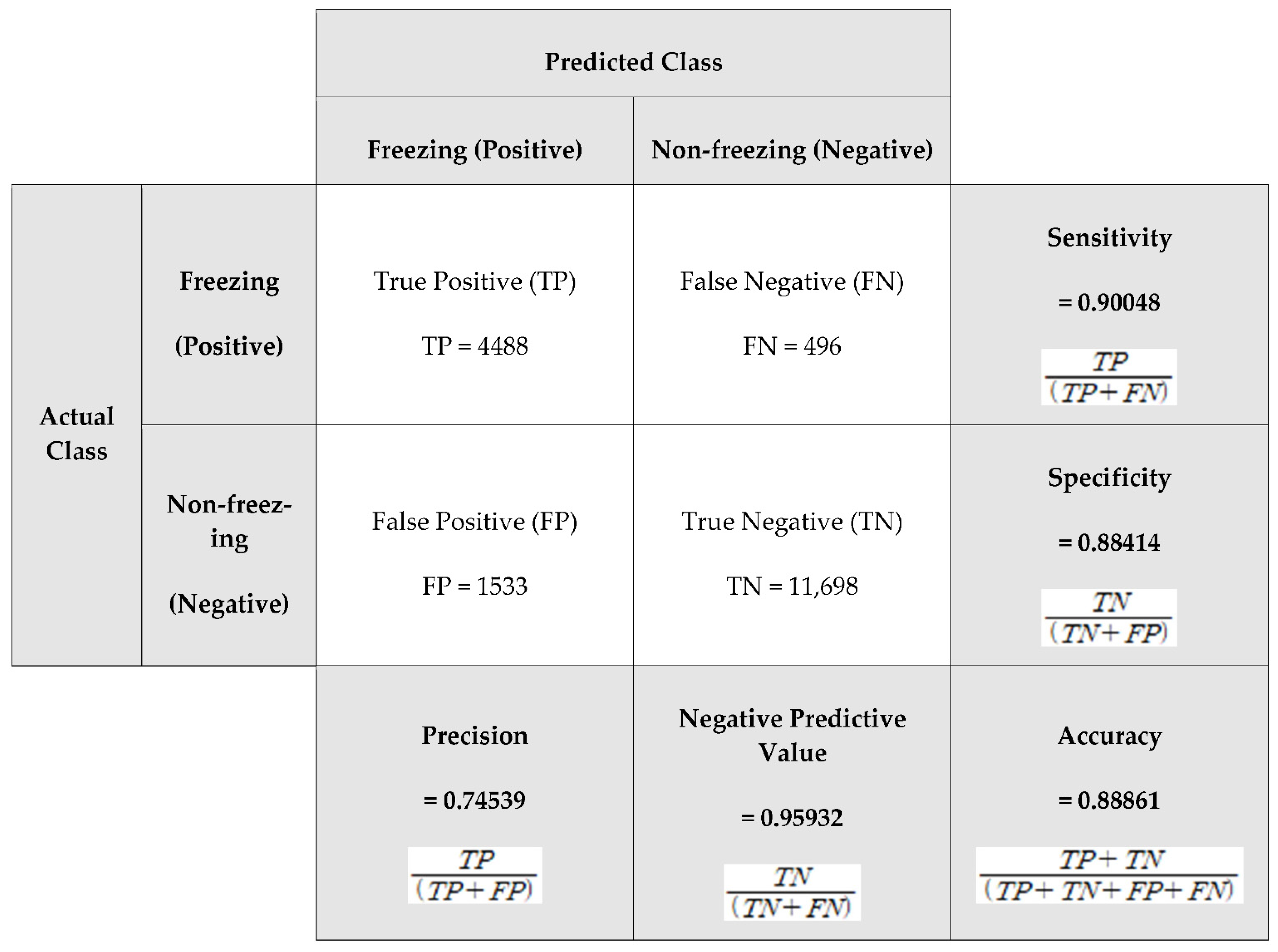
  29. Stehman, S.V. Selecting and interpreting measures of thematic classification accuracy. Remote Sens. Environ. 1997, 62, 77–89. [Google Scholar] [CrossRef]
  30. Korea Meteorological Administration. Numerical Forecasting Is Responsible for Meteorological and Climate Industries; Korea Meteorological Administration: Seoul, Republic of Korea, 2013; p. 17. [Google Scholar]
  31. Lindberg, F.; Holmer, B.; Thorsson, S. SOLWEIG 1.0—Modelling spatial variations of 3D radiant fluxes and mean radiant temperature in complex urban settings. Int. J. Biometeorol. 2008, 52, 697–713. [Google Scholar] [CrossRef] [PubMed]
  32. Lindberg, F.; Grimmond, C. The influence of vegetation and building morphology on shadow patterns and mean radiant temperature in urban areas: Model development and evaluation. Theor. Appl. Climatol. 2011, 105, 311–323. [Google Scholar] [CrossRef]
  33. Lindberg, F.; Onomura, S.; Grimmond, C.S.B. Influence of ground surface characteristics on the mean radiant temperature in urban areas. Int. J. Biometeorol. 2016, 60, 1439–1452. [Google Scholar] [CrossRef] [PubMed]
  34. Yi, C.; Kwon, H.G.; Lindberg, F. Radiation flux impact in high density residential areas. J. Korea Assoc. Geogr. Inf. Stud. 2018, 21, 40–46. [Google Scholar] [CrossRef]
  35. Yang, H.J.; Yi, C.Y.; Bae, M.K. The analysis of road surface characteristics for road risk management in heat wave: Focused on Cheongju City. J. Environ. Policy Adm. 2019, 27, 51–73. [Google Scholar] [CrossRef]
  36. Hsu, C.Y.; Ng, U.C.; Chen, C.Y.; Chen, Y.C.; Chen, M.J.; Chen, N.T.; Lung, S.C.C.; Su, H.J.; Wu, C.D. New land use regression model to estimate atmospheric temperature and heat island intensity in Taiwan. Theor. Appl. Climatol. 2020, 141, 1451–1459. [Google Scholar] [CrossRef]
  37. National Spatial Data Infrastructure Portal. Available online: http://data.nsdi.go.kr (accessed on 1 October 2020).
  38. Environmental Geographic Information Service, Korean Ministry of Environment. Available online: https://egis.me.go.kr (accessed on 10 October 2020).
  39. Guan, K.K. Surface and Ambient Air Temperatures Associated with Different Ground Material: A Case Study at the University of California, Berkeley. Surf. Air Temp. Ground Mater. 2011, 196, 1–14. [Google Scholar]
  40. Bogren, J. Screening effects on road surface temperature and road slipperiness. Theor. Appl. Climatol. 1991, 43, 91–99. [Google Scholar] [CrossRef]
  41. Kim, Y.J.; Kim, B.J.; Shin, Y.S.; Kim, H.W.; Kim, G.T.; Kim, S.J. A case study of environmental characteristics on urban road-surface and air temperatures during heat-wave days in Seoul. Atmos. Ocean. Sci. Lett. 2019, 12, 261–296. [Google Scholar] [CrossRef] [Green Version]
  42. Karsisto, V.; Nurm, P. Using car observations in road weather forecasting. In Proceedings of the 18th International Road Weather Conference, Fort Collins, CO, USA, 27–29 April 2016. [Google Scholar]
  43. Tegegne, E.B.; Ma, Y.; Chen, X.; Ma, W.; Wang, B.; Ding, Z.; Zhu, Z. Estimation of the distribution of the total net radiative flux from satellite and automatic weather station data in the Upper Blue Nile basin, Ethiopia. Theor. Appl. Climatol. 2021, 143, 587–602. [Google Scholar] [CrossRef]
  44. Bell, M.; Ellis, H. Sensitivity analysis of tropospheric ozone to modified biogenic emissions for the Mid-Atlantic region. Atmos. Environ. 2004, 38, 1879–1889. [Google Scholar] [CrossRef]
Figure 1. Study area: (a) South Korea; (b) Seoul metropolitan area (SMA); (c) satellite image, extracted LDAPS grid point locations; and (d) street/route view of the study area (Source: Kakao).
Remotesensing 14 06379 g001
Figure 2. Road-freezing decision tree algorithm according to [23].
Remotesensing 14 06379 g002
Figure 3. Road-freezing evaluation via the confusion matrix.
Remotesensing 14 06379 g003
Figure 4. Diurnal variations in the air, dew point, and road surface temperatures on the selected days based on the observations and potential road-freezing section (sky blue color) calculated according to the algorithm of [23]. (a) 24 January, (b) 25 January, (c) 10 February, and (d) 11 February.
Remotesensing 14 06379 g004
Figure 5. Comparison of diurnal variations in temperature, dew point temperature, and solar radiation between the LDAPS-predicted and meteorological station observations on the four selected days: (a) 25–26 January; and (b) 10–11 February 2021.
Remotesensing 14 06379 g005
Figure 6. Input land surface data for the study area (yellow lines indicate roads): (a) digital surface model (DSM); (b) canopy digital surface model (CDSM); (c) land cover (LC).
Remotesensing 14 06379 g006
Figure 7. Meteorological observation station (a) and equipment composition (b) and its immediate surroundings in the (c) north and (d) south direction.
Remotesensing 14 06379 g007
Figure 8. Flowchart of the study process.
Remotesensing 14 06379 g008
Figure 9. (a) Risk level 1–5 due to shadow effect. The white circle is the observation site where the picture on the right was taken. Road shadows captured from 12:09 (b) and 12:39 (c) on 21 January 2021, by the observation station (the up-lane is closer to the camera, while the down-lane is located closer to the top of the photo).
Remotesensing 14 06379 g009
Figure 10. Comparison of diurnal variations in solar radiation between the surface (meteorological station) observations, SOLWEIG, and LDAPS for each of the selected days (a) 25 January, (b) 26 January, (c) 10 February and (d) 11 February 2021.
Remotesensing 14 06379 g010
Figure 11. Scatter plots between modeled (SOLWEIG) and observed Kdown values during the entire study period (a) and for freezing-time and (b) observations.
Remotesensing 14 06379 g011
Figure 12. Surface temperature distribution calculated from satellite imagery and daytime upward longwave radiation distribution.
Remotesensing 14 06379 g012
Figure 13. Scatter plots between modeled (SOLWEIG) and observed Kdown values (a) during the entire study period and (b) for freezing.
Remotesensing 14 06379 g013
Table 1. SOLWEIG land cover classification and corresponding parameters [33].
NameCodeAlbedo (α)Emissivity (ε)Ts/η max (°C)Tstart (◦C)TmaxLST
(Local Time, h)
Cobble_stone_2014a00.200.950.37−3.4115.00
Dark_asphalt10.180.950.58−9.7815.00
Roofs (buildings)20.180.950.58−9.7815.00
Evergreen30.160.940.21−3.3814.00
Deciduous40.160.940.21−3.3814.00
Grass_unmanaged50.160.940.21−3.3814.00
Bare_soil60.250.940.33−3.0114.00
Water70.050.980012.00
Table 2. Configuration of observation equipment, measurement, and error range.
ObservationResolutionRangeError Range
Wind direction0~360°±3°
Wind speed0.1 m/s0~67 m/s±5%
Temperature0.1 °C−40~65 °C±0.5 °C
Relative humidity1%0~100%±3%
Dew point0.1 °C−76~54 °C±1.5 °C
Precipitation0.2 mm0~6553 mm±4%
Pressure
(Altitude range—600~4750 m)
0.1 mmHg
0.1 mb
410~820 mm
Hg540~1100 mb (hPa)
±0.8 mmHg ± 1.0 mb
(hPa)
Solar radiation1 w/m20~1800 w/m2±5%
Surface temperature1 °C−40~65 °C±0.5 °C
Surface condition12 MP, Day and nighttime lapse
Table 3. Thirty-minute trends of the up- and down-lane shadow pattern effects, mean shadow pattern values, and the Level 1:5 ratios for 21 January 2021.
Shadow PatternUp-LineDown-Line
Up-LineDown-LineAverageLevel 1 (%)Level 5 (%)Level 1 (%)Level 5 (%)
8:000.0000.0000.0000.000.000.000.00
8:300.0440.0420.0434.3595.654.1595.85
9:000.2960.2390.26929.3570.6523.3776.63
9:300.5520.3980.47154.6845.3238.6461.36
10:000.8140.5960.69780.9419.0658.5341.47
10:300.8460.6140.72184.1715.8360.3739.63
11:000.8550.6160.72485.0314.9760.5039.50
11:300.8600.6130.72785.5514.4560.2439.76
12:000.8370.6000.71183.2516.7558.9241.08
12:300.8270.5980.70382.1917.8158.7241.28
13:000.8230.5980.70181.7318.2758.6641.34
13:300.7890.5810.66778.2321.7756.9543.05
14:000.7310.5500.62872.2327.7753.7946.21
14:300.6750.5090.58666.6933.3149.9750.03
15:000.5900.4320.50158.0541.9542.1357.87
15:300.5040.3690.42749.7450.2636.0863.92
16:000.3390.2820.30533.5866.4227.7272.28
16:300.1300.1240.12512.7387.2711.9888.02
17:000.0000.0000.0000.000.000.000.00
17:300.0000.0000.0000.000.000.000.00
Table 4. Mean shadow pattern values, SVFbuilding-ground, and SVFvegetation for each level of shadow pattern on the up- and down-lanes.
Shadow Pattern LevelLane12345
Shadow pattern valueUp0.8000.6710.4860.2860.078
Down0.8020.6720.4830.2740.037
SVFbuilding-groundUp0.9370.9430.9280.9270.927
Down0.9450.9550.9240.9170.909
SVFvegetationUp0.9680.9350.8830.8790.832
Down0.9780.9650.8570.5900.403
Publisher’s Note: MDPI stays neutral with regard to jurisdictional claims in published maps and institutional affiliations.

