Abstract
Inter-satellite links (ISLs) can improve the performance of the Global Navigation Satellite System (GNSS) in terms of precise orbit determination, communication, and data-exchange capabilities. This research aimed to evaluate a simulation-based processing strategy involving the exploitation of ISLs in orbit determination of Galileo satellites, which are not equipped with operational ISLs. The performance of the estimation process is first tested based on relative weighting coefficients obtained with methods of variance component estimation (VCE) varying in the complexity of the calculations. Inclusion of biases in the ISL measurements allows evaluation of the processing strategy and assessment of the impact of three different sets of ground stations: 44 and 16 stations distributed globally and 16 located in Europe. The results indicate that using different VCE approaches might lower orbit errors by up to 20% with a negligible impact on clock estimation. Depending on the applied ISL connectivity scheme, ISL range bias can be estimated with RMS between 10% to 30% of initial bias values. The accuracy of bias estimation may be associated with weighting approach and the number of ground stations. The results of this study show how introducing VCE with various simulation parameters into the processing chain might increase the accuracy of the orbit estimation.
1. Introduction
Inter-Satellite Links (ISLs) allow for data exchange and provide precise pseudorange measurements between satellites in a specific constellation. ISLs intend to improve the positioning accuracy and orbit determination in Global Navigation Satellite Systems (GNSS), also time transfer and autonomous orbit determination performed on board the navigation satellites [1,2,3,4,5,6,7,8,9]. Connections between satellites can be used to transfer information, which might shorten the ephemeris update interval and enhance navigation [10]. The ISL system usually establishes links outside of the atmosphere, eliminating atmospheric effects, and it is also less impacted by multipath and interference than GNSS measurements [11]. Introducing ISLs to orbit determination could reduce the number of the ground stations required for orbit determination. The stations should be positioned around the world as optimally as possible; however, this is not always possible because of geographic or political reasons. Several studies into the impact of station distribution while ISLs are working have been conducted [12,13,14,15,16,17,18,19]. The main findings of these works are that ISLs can considerably improve orbit determination, can help to reduce the number of ground stations exploited in the processing, and help in better clock error estimation. ISLs might be an essential part of other constellations, e.g., consisting of Low Earth Orbits (LEO) satellites.
At present, the BeiDou Navigation Satellite System is the most advanced navigation system to integrate ISLs [10,20,21,22,23,24]. The ISL payload enables observation of other satellites and ground stations with Ka-band single frequency pseudorange measurements [5,22,25,26,27,28]. Each satellite operates within a 1.5 s timeslot with another satellite, creating a link pair [5,27]. The BeiDou constellation orbits and clock offsets are estimated simultaneously [29]. This generation of satellites can realize autonomous navigation (Auto-Nav). However, even with additional ISL measurements, the constellation is still affected by external environmental and technological effects [5,25]. The ISL payload allows observation of other satellites and ground stations with Ka-band single-frequency pseudocode ranging measurements [5,25,26,27]. In the BeiDou constellation, autonomous orbit determination with the on-board ISLs payload is conducted with additional anchor stations to suppress any relative motion of the constellation. Measurements between satellites and anchor stations, described as ground–satellite links (GSLs), use the same communication and measurement system as ISLs [25].
ISLs have been only thoroughly tested in orbit in the BeiDou constellation, but they are considered to be a fundamental component of the future Galileo constellation. According to a statement published on the European Commission webpage, a new generation of Galileo satellites is under development [30]. Among the many new capabilities relying on original technologies (e.g., new atomic clock technologies and use of full electric propulsion systems), the integration of ISLs is also planned. A demonstration flight and verification of the ISLs on board a Galileo 2nd Generation spacecraft is planned for 2024 [30]. Simulation studies have been performed to assess the impacts of including ISLs in Galileo, focusing on the use of the ISL in orbit determination and clock estimation, as well as for time transfer purposes and possible extension with LEO satellites [3,12,31,32,33,34,35]. The main findings of these works are that ISL enhance the orbit and clock prediction accuracy and reduce the dependency from ground stations. In the simulation studies also the advantages of optical two-way inter-satellite links for orbit determination is discussed, showing potential improvements in accuracy compared to microwave links. Such connections will also help in time transfer and clock synchronization. Moreover, potential future system with optical ISL and optical frequency references called Kepler, was proposed by the German Aerospace Center. Such system topology might effectively reduce modelling errors in the Earth parameters. It is expected that Kepler improve global geodetic reference frames with the focus on the Earth rotation parameters. However, the evaluation of the relative weighting of different measurement techniques taking part in orbit determination should be conducted, including also testing various settings and properties of observations.
In this simulation study, we focus on introducing ISLs in the orbit determination of a Galileo-like constellation together with GNSS measurements and relative weighting of both types of measurements. We are interested in the analysis of different processing solutions depending on the choice of ground station set, weighting approaches, or connectivity scheme. We used three sets of GNSS ground stations and four ISL connectivity schemes for which we exploited methods of relative weighting based on variance component estimation (VCE) together with two values of ISL range bias. We present the impact of weighting properties on accuracy of orbit determination with reference to the number of ground stations and ISL range bias estimation depending on the connectivity scheme. This study aimed to address the following questions: (1) how the choice of VCE approach impacts the orbit and clock estimations, (2) how the weighting approach affects bias estimation, and (3) how the weighting approach and bias might change the estimation results with various sets of ground stations comparing to GNSS-only solution (i.e., without support of ISLs). The outcomes of this research might be useful in establishing future processing schemes for combined orbit determination supported with ISLs.
The remainder of this paper is organized as follows: in Section 2 the methodology of the simulation is described, including observation models, ISL connectivity schemes, simulation properties, and a detailed description of the VCE methods. In Section 3 we assess the VCE approaches, results of ISL range bias estimation, and impact of the number of stations on both, i.e., weighting and the bias estimation with reference to the GNSS-only solution. In Section 4 we discuss the results in terms of possible processing strategies of relative weighting and ISL range bias estimation, and we conclude the paper.
2. Methodology
2.1. Observation Models
In our research, the ISL and GNSS measurements are both simulated as geometric distances between satellite positions or between a satellite and a ground station. The ranging errors are assumed to be zero-mean Gaussian white noise with selected standard deviations (marked as σ), which are added to geometric distances. This allows the simulation of various behaviors of the ISLs and GNSS ranges for each simulation scenario. Both ISL and GNSS measurements are also deteriorated by satellite-only or satellite and station clock errors, respectively. Clock errors were also simulated as white noise with defined standard deviation. In addition, ISL measurements are burdened with bias that is simulated as a constant value for each satellite per day. A more detailed description of the simulation parameters is presented in Section 2.2.
In our simulation, we considered two types of possible connection between satellites (Figure 1) [12,34]:
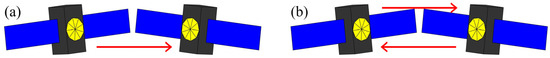
Figure 1.
Connection type: (a) one-way and (b) dual one-way [12,34].
- One-way–satellite establishes a link with satellite (i.e., one range measurement at a time), and
- Dual one-way–satellite establishes a link with satellite and satellite establishes a link with satellite (i.e., two range measurements at a time).
The ISL pseudorange can be written as follows [12,34]:
where and represent the three-dimensional position of satellites i and j, respectively, in Cartesian coordinates; and are the clock errors of the satellites; c is the speed of light; is the signal travel time; and are the ISL range biases; and, ε is the noise of the measurements. The emission time is given by the clock of the satellite that transmits in the current epoch and the reception time is given by the clock of the receiving satellite.
Equation (1) represents the one-way measurement type and requires a satellite clock error estimation. In dual one-way ISLs, the two satellites send signals to each other in turn [5,36]. The dual one-way observations need to be transformed to a common epoch for the satellite orbit determination, ensuring that the distance between two satellites is reduced to the same observation time, . The mean value computed from and , given in Equation (2), contains only orbital parameters and biases, and the satellite clock error is eliminated:
Exploitation of simultaneous dual one-way measurements is free of clock offsets and might be used to determine the orbit [37,38].
For simulation of ground station–satellite measurements we used the following model:
where and are three-dimensional position of the stations and satellites in Cartesian coordinates, and are the clock errors of the satellites, is the zenith wet delay (ZWD), and is the noise of the measurements. We do not consider zenith hydrostatic delays. The GNSS measurements are simulated as unambiguous carrier phases with a priori determined accuracy.
2.2. Connectivity Schemes
There are many ways to establish satellite pairs and then assign ISLs between satellites in measurement epochs, i.e., satellite pairs choice may change in each epoch. In our research, this ranging schedule is called a “connectivity scheme”. In our previous studies, we stated that the choice of connectivity scheme does not have a major impact on orbit determination and clock estimation unless observation conditions are not optimal (e.g., measurement accuracy and interval, or the number of ground stations) [12,34]. However, the choice of connectivity scheme is still important to maximize efficiency of the connections and meet data-exchange requirements [39,40]. It is also important in the case of mixed constellation configurations of geostationary orbit (GEO), inclined geostationary orbit (IGSO), and medium earth orbit (MEO) satellites (e.g., the BeiDou configuration [41]).
The ISL observation strategy is based on the satellite pairs; satellites establish connections during predefined time slots according to the chosen connectivity scheme. Satellite pairs can change from epoch to epoch (dynamic schemes), or the connection can be kept for several measurement epochs (static schemes). Connectivity schemes might also be defined based on geometric information about satellites, the distances between them, or the pointing angles of the ISL system [42], and the selection of algorithms that maximize network connectivity and improve network performance [39,43,44,45,46,47,48].
Mutual visibility is very important for establishing connections between satellites in each of the measurement epochs, as ISLs cannot be maintained permanently during the whole system period because of temporary losses of visibility [42]. Technological limitations of the measurements (e.g., distance, azimuth, and elevation) could affect the ISLs [49] but the main obstructions to establishing connections between satellites are the Earth and atmosphere, for which the height that affects the satellite links is defined as 1000 km [50,51]. In our simulations, links crossing the atmosphere are not considered as a pair to connect the satellites.
We applied two types of connectivity schemes: intra-plane and sequential, which were used in our previous research [12,34]. The intra-plane scheme is created on the basis of the slot of the satellites in the orbital plane. In intra-plane closed configuration all satellites in the same orbital plane are connected, whereas in intra-plane open configuration, one connection between adjacent satellites is missing. The intra-plane schemes use one-way connection type. The sequential scheme consists of observation scenarios based on a sequence of measurements defined a priori [3,11,12,34].
2.3. Simulation Properties
This research is based on simulations made with the General Simulation Tool for Earth-Orbiting Objects (GSTE) software, written by Maciej Kalarus during his work at Centrum Badań Kosmicznych Polskiej Akademii Nauk (CBK PAN) and developed for the ISL by Tomasz Kur. The key software modules include an orbit propagator with specific support for navigation satellites, a simulator of the GNSS and the ISL observations, and a parameter estimator based on weighted least squares (WLS) method with use of 4 iterations. The GNSS measurements and ISL observations were simulated based on a Galileo-like constellation (Table 1). Reference orbits were propagated using a set of gravitational and non-gravitational force models (Table 1). To obtain reliable results, each simulation scenario was repeated 10 times with randomly generated errors (i.e., measurement precision) imitating the principles of the Monte Carlo method, to provide more reliable error assessment under various simulation conditions. In the plots presenting orbit and clock estimation errors, we display mean RMS error values from the repetitions together with their standard deviations. It should be noted that estimated corrections using real data depend on many models and parameters such as tidal motion [52], antenna phase center offsets, and satellite attitude, which are not discussed in this study (the simulations are simplified and do not consider these errors in the included models). Three sets of GNSS ground stations were used (Figure 2): 16 stations located globally, 44 stations located globally, and 16 placed only in Europe. The 16-station global set partially represents Galileo Sensor Station used in previous research [32,33]. Regional stations located in China only with ISLs support were also tested for the BeiDou navigation system with promising results [17,18,19]. ISLs in BeiDou compensate for the lack of satellite visibility from a ground station and help to measure the relative inter-satellite clock in nearly real time. ISL observations help in accurate orbit determination of a small regional network comparable with the global network. Additionally, ISL is integrated with observations from regional stations for broadcast clock estimation. The clock errors between satellites are obtained through centralized estimation based on ISLs.

Table 1.
Simulation and estimation settings.
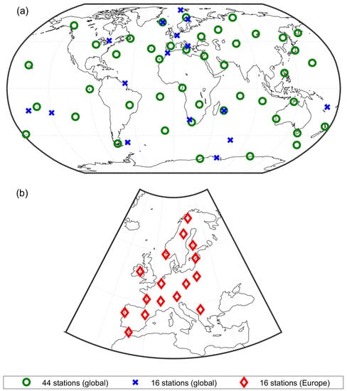
Figure 2.
Location of the GNSS ground stations used in the simulations, shown on the two maps for better readability: (a) 44 and 16 stations placed globally, and (b) 16 stations in Europe.
2.4. Variance Component Estimation
Observation methods characterized by different technologies and background devices (e.g., electronic systems) vary in measurement accuracy and noise or presence of systematic errors. In some cases, the use of a priori adopted values for weighting might not be beneficial. When combining several observation types for the further estimation of parameters, it is worth considering the relationship between the observation errors, which are probably distinct between each observation technique [57]. As a result, variance estimation methods have emerged to optimally estimate variance and covariance components. VCE is an algorithm that recognizes the relative contribution of measurements of each type or selected partial results in the final solution [58].
The VCE is used in the calculation of the gravity field models for weighting individual satellite passes or monthly solutions of gravimetric missions [59]. The VCE is also exploited in the kinematic orbit determination, where posteriori variances are obtained for different types of GNSS observations to eliminate erroneous measurements [60]. In estimating precise orbits, the VCE method allows the detection of outliers, and the weighting factors can be obtained for individual satellites in each epoch [59]. The VCE method is also used in static and kinematic single point positioning [61,62,63]. The VCE method can also be applied in a combined solutions used for the realization of a terrestrial reference system [64,65]. The obtained weighting coefficients are used in scaling the covariance matrices of individual solutions before their combination. In addition, VCE can be used in data fusion during parameter estimation and satellite orbit determination using ISL measurements [15].
In our research, the WLS method is performed iteratively to determine orbit. The VCE method is usually applied in the last iteration of WLS and is also performed iteratively until the convergence criterion of the VCE algorithm is met [61,62,66]. A convergence criterion can be set for given parameters or for the weighting factor values obtained by the VCE. There are several approaches to the implementation of the VCE method, but in this study, we focus on the Helmert approach [61,62,64,67] and Förstner approach [57,59,61]. The VCE algorithm was applied as follows:
Step 1. In iteration , normal equations matrices for GNSS measurements () and ISL () are computed with the assignment of weighting coefficients and equal to a priori measurement noise and , respectively:
Step 2. The sum of weighted normal matrices is computed:
Step 3. In iteration new weighting coefficients and are determined according to the selected approach, where means number of observations for each respective measurement technique:
- Helmert approach
- Förstner approach
Step 4. Check the assumed convergence criterion :
Step 5. If the criterion is not met, then new sum of normal matrices for both types of observations is computed with use of new weighting coefficients and then Step 3 and Step 4 are repeated until the criterion is met.
The VCE is used in the last iteration of WLS adjustment, while in previous iterations, observation weights are used based on the noise of measurements (see details in Table 1). When weighting coefficients and are both equal to 1 (therefore only weighting with a priori noise is used) then this approach is called Nominal weighting in this research. It is used for comparison purposes and is not recognized as the VCE method in the research. Each VCE approach uses a priori measurement noises and number of observations for each technique. Additionally, we consider the correlations between GNSS and ISL techniques as negligible for research purposes. In the simulations presented in the research, it should be noted that the number of GNSS observations might outnumber the ISLs and that GNSS observations substantially contribute to the orbit solution, as a significant number of GNSS observations is used during determination of weighting coefficients. A comparison of the number of observations is presented in Table 2.
Table 2.
Number of GNSS and ISL measurements for 1 day.
3. Results
3.1. Comparison of the VCE Approaches
Numerous versions of the VCE are available, depending on the problem requiring relative weighting. This section aims to compare the VCE approaches described in Section 2.4: Helmert which might be considered as a strict solution, and Förstner, a simplified version of Helmert approach. The idea of relative weighting of ISL and GNSS in a Galileo-like needs to be examined in the case of complexity of joining two various techniques for orbit determination. A strict solution would be more precise in assigning weighting coefficients but might be more computationally expensive. We simulated six scenarios to conduct a comparison of the following approaches: Förstner, Helmert, and Nominal with 44 and 16 ground stations with global distribution (Table 3). The scenario names given in Table 3, also used in the figures, were created based on the following scheme: {number of stations and their placement}-{ISL range bias value in cm}-{VCE approach}, where G is global, E is Europe, F is Förstner, H is Helmert, and N is Nominal.
Table 3.
Summary of the simulation scenarios used for comparison of the VCE approaches.
The weighting coefficients obtained for selected simulation scenarios are presented in Table 4. The differences between Helmert and Förstner approaches are mostly negligible for the same number of ground stations. A comparison of the connectivity schemes for the weighting coefficients indicates that sequential schemes are less sensitive to a limited number of stations as the changes in the coefficient are relatively smaller than those in intra-plane schemes. However, the intra-plane schemes have higher values of the coefficients with 44 stations and the weighting coefficient values decrease for 16 stations. In our simulations, GNSS observations have a considerable effect on the solution. Intra-plane schemes due to lack of links between the orbital planes are more dependent on the number of GNSS measurements what relates to the number of ground stations. Comparison of two connection types reveals that dual one-way is considered as a better solution due to higher values of weighting coefficient. Sequential one-way has lower values of coefficients than sequential dual one-way probably because of taking part in satellite clock estimation. Sequential schemes seem to be more dependent on the connection type than on the VCE approach. Intra-plane schemes are characterized by constant pairs and one-way connection type, and they have higher or similar values of weighting coefficients than sequential one-way. Considering just weighting coefficients, it might suggest that intra-plane schemes are more reliable than sequential one-way, i.e., static schemes using the same connection type as sequential schemes might better contribute to orbit and clock estimation.
Table 4.
Value of VCE weighting coefficients obtained for normal equations for GNSS and ISL.
The results of the orbit determination are presented in Figure 3. The values of weighting coefficients might not have a substantial impact on errors of estimated parameters. The radial component in Figure 3a is the least sensitive on choice of different simulation settings as the results are very similar for all simulation scenarios (range of RMS is from 0.3 cm to 0.6 cm). The impact of various simulation settings is more visible in errors for the along-track and cross-track components. While considering the impact of VCE approach, usually the Helmert method is best, followed by Förstner and Nominal, but the differences between them are very small, i.e., less than 0.2 cm for sequential schemes and up to 0.4 cm for intra-plane schemes. The choice of connectivity scheme can determine the method performance, i.e., results for sequential schemes are more homogenous with the Helmert approach across different scenarios than for intra-plane schemes. For sequential schemes, the choice of VCE approach is not important when 44 ground stations are used (Figure 3d). For the combination of 16 stations and intra-plane schemes, there are modest differences between weighting methods, in favor of the Helmert. For sequential dual one-way scheme, the Förstner approach would be the best choice of VCE method as the orbit errors with 16 stations located globally are slightly lower than for the Helmert approach. For most scenarios, using the Helmert approach gives no more than about 20% improvement in orbit accuracy compared with the Förstner approach, especially when the ISL connectivity scheme is not dynamic (e.g., in intra-plane schemes). Improvement is more noticeable for Förstner or Helmert in relation to Nominal weighting. The difference between extreme values of RMS orbit errors obtained from repeated simulations can reach 20–30% of mean values. It is also worth mentioning that in tested cases the Helmert and Förstner approaches are sensitive to the number of GNSS observations. When 16 stations were used, the standard deviations of solutions are larger than with use of 44 ground stations, but still smaller than for Nominal weighting in respective settings.
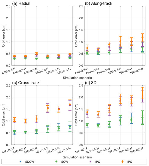
Figure 3.
Comparison of the Helmert and Förstner approaches with Nominal and their impact on orbit estimation mean RMS errors for (a) radial, (b) along-track, (c) cross-track components, and (d) the total 3D RMS value. The simulation scenario names are given in Table 3.
There is a very slight improvement in clock estimation errors for Helmert and Förstner approaches for satellite clocks when using 44 ground stations (Figure 4) compared to Nominal (it is less than 0.01 ns for all connectivity schemes). There is also no notable difference between Nominal and Förstner and between Nominal and Helmert for use with measurements for 16 stations. The results presented in Figure 4 suggest no direct impact of the weighting method on clock estimation results in our simulation methodology. Considering orbit and clock estimation outcomes, the impact of choice of VCE approach between Helmert and Förstner also seems to be negligible. For further analysis, we decided to use the Förstner approach, as it is the simpler solution with comparative results to Helmert approach.
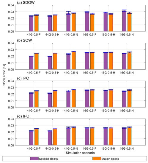
Figure 4.
Mean RMS estimation errors for satellite and station clocks considering the station set and VCE approach with respect to connectivity scheme: (a) SDOW, (b) SOW, (c) IPC, and (d) IPO. The simulation scenario names are given in Table 3.
3.2. ISL Range Bias Estimation against Weighting Approach and Ground Station Sets
3.2.1. Orbit Estimation Errors
It is expected that the ISL technique will be charged with systematic errors derived from hardware devices, i.e., antennas, electronics, and the measurement system, which we will describe as “ISL range biases”. Here, we do not investigate the origins of these biases in detail. We instead show the impact of ISL range bias values and their estimation for different ground station sets from the perspective of the choice of weighting approach. The simulations were conducted for an ISL range bias equal to 0 cm (no bias is simulated and estimated) and when ISL range bias is equal to 0.5 cm and 1.0 cm to check the general impact of the ISL range biases on satellite positions. A detailed description of the simulation scenarios used for orbit estimation errors analysis is given in Table 5. Simulations assuming ISL range bias equal to 0.5 cm are used to evaluate the impact of ground station set in a next subsection. These scenario names are created as follows: {number of stations and their placement}-{ISL range bias value in cm}-{VCE approach}, where G is global, E is Europe, F is Förstner, and N is Nominal.
Table 5.
Summary of simulation scenarios used for the ISL range bias estimation check.
In Figure 5 we demonstrate orbit errors in each component for the different ground station sets according to scenarios described in Table 5. As shown in Section 3.1, for globally distributed stations and confirmed here, the relation between the Förstner and Nominal weighting is preserved regardless of the bias presence, i.e., Förstner outperforms Nominal. In each component, the same relation is shown between ISL range bias value and weighting method, i.e., using Förstner approach in most cases helps to reduce the error, especially in the along-track component (Figure 5b). The visible impact of bias is apparent in errors for the cross-track component (Figure 5c) for globally distributed stations and for intra-plane schemes. The error bars are slightly larger by about 10% of the mean orbit errors in along-track component (Figure 5b) and cross-track (Figure 5c) when ISL range bias is estimated. However, estimation errors in cross-track component affect the 3D errors the most. The lowest 3D errors at the level of 0.8–0.9 cm are obtained for sequential schemes with 44 ground stations.
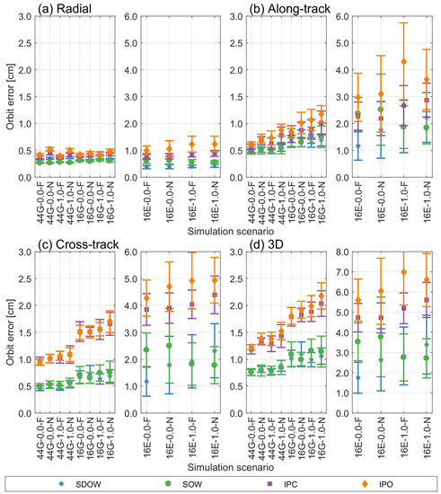
Figure 5.
Comparison of weighting method with reference to ground station set and bias value used in simulations to analyze the impact on mean RMS errors in the orbit estimation for (a) radial, (b) along-track, (c) cross-track components, and (d) the total 3D RMS value. The simulation scenario names are given in Table 5. Because of the higher errors, results for the simulation scenarios with 16 stations in Europe are shown on a separate plot with a different range on the vertical axis.
The situation changes for the 16 stations positioned in Europe. In Figure 5d, with total 3D values of orbit errors for ground stations in Europe, the weighting method affects the estimation results differently for each of the connectivity schemes. For intra-plane closed scheme Förstner approach helps to reduce errors, while for intra-plane open scheme Nominal weighting has lower 3D errors than Förstner approach. However, Förstner approach helps to lower total errors in sequential dual one-way. On the contrary, for sequential one-way the choice of VCE approach is not impactful. Looking at total orbit error (Figure 5d), 16 stations (positioned either globally or regionally) cannot ensure repeatability of solutions obtained from a series of simulations for each connectivity scheme as computed errors are ±25% of the mean orbit error obtained for each simulation scenario. Thus, relatively small changes in e.g., measurement accuracy might impact the orbit estimation error.
3.2.2. ISL Range Bias Estimation
Figure 6 shows the effect of the weighting method and connectivity scheme when the value of the simulated ISL range biases is 1.0 cm. Estimation errors of ISL range bias estimation equal to 0.5 cm are shown in Figure A1 in Appendix A. For simulated ISL range bias values and for each ground station set we can distinguish the impact of the satellite placement on the orbital plane, especially for intra-plane schemes when 16 stations are used. However, increasing the number of ground stations to 44 for orbit determination does not considerably improve the bias estimation, i.e., the choice of connectivity schemes has a higher impact on the results than station set. Connectivity schemes with invariable geometry such as intra-plane schemes might not be beneficial or additionally burdened with systemic errors. It is seen in Figure 6b,c where ISL range bias estimation for intra-plane open is affected by systematic error which degrades the mean solution by about 0.4 cm compared to simulated 1 cm bias. Due to geometrical properties of intra-plane open (i.e., missing link), erroneous ISL range bias estimation for one satellite might more affect other satellites on the same orbital plane than it is in case of sequential schemes. Initial values of calibration constants or fixing the ISL range bias value for chosen satellites might improve the ISL range bias estimation in this case, but it needs further testing. We would like to address these questions for next research involving more deeply wide range of possible methods to handle range biases in parameter estimation, including calibration. In terms of the influence of the weighting method and considering all simulation scenarios, the results with the smallest difference among the scenarios are obtained for the sequential dual one-way scheme. The most variable bias results occur for the intra-plane open (±20% of base value) and sequential one-way schemes.
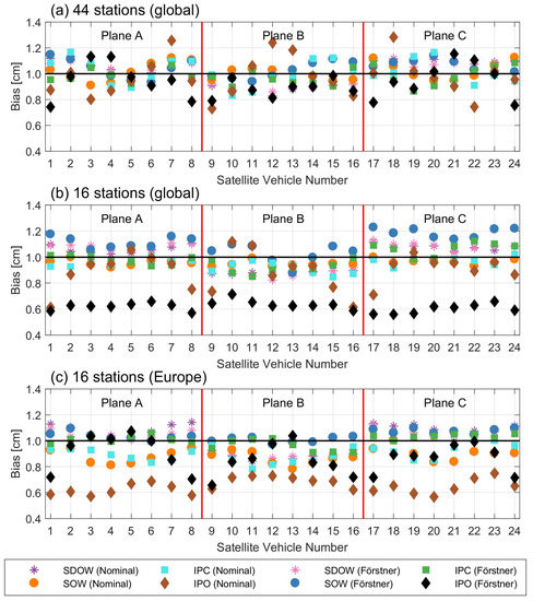
Figure 6.
Mean estimated ISL range biases of each satellite (simulated value of 1.0 cm) for different ground station sets: (a) 44 stations (global), (b) 16 stations (global), and (c) 16 stations (Europe) under different weighting methods. Please note the scale on the vertical axis.
Statistical measures presented in Table 6 are computed with distinction to the weighting method and connectivity schemes, but regardless of the ground station set. It means that these values show general possibilities of ISL range bias estimation in applied processing, including presence of systemic errors visible in Figure 6b,c. The RMS is similar for sequential dual one-way and sequential one-way schemes for both types of weighting. For intra-plane schemes the RMS values are higher Nominal than in Förstner weighting. The range of ISL range bias differences is also wider for Nominal weighting. The choice of sequential scheme and ground station set is more crucial for accurate ISL range biases estimation. The distribution of differences between simulated and estimated biases with reference to the ground station sets and weighting approach is shown in Figure 7. The differences are computed for ISL range biases equal to 0.5 cm and 1.0 cm. Förstner method performs better in ranges from −0.2 cm to 0.2 cm for the global station distribution than Nominal weighting (the number of differences in this range is higher in Förstner than Nominal) and the extreme differences are also smaller with the Förstner than in Nominal weighting. Direct comparison of Figure 7b,d,f reveals that a lower number of stations and thus a smaller number of GNSS measurements still allows for accurate bias estimation. The lowest RMS of estimated bias is noticed for sequential dual–one-way scheme regardless of weighting approach or ISL range bias values.
Table 6.
Statistics of differences between simulated and estimated values of biases with reference to weighting and connectivity schemes. Presented values are computed for all simulation scenarios with estimated ISL range bias (regardless the ground station set).
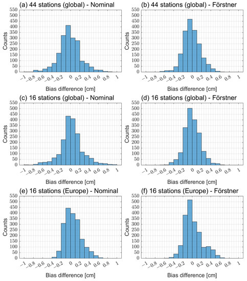
Figure 7.
Histograms of ISL range bias differences for (a) 44 stations (global) with Nominal weighting, (b) 44 stations (global) with Förstner weighting, (c) 16 stations (global) with Nominal weighting, (d) 16 stations (global) with Förstner weighting, (e) 16 stations (Europe) with Nominal weighting, and (f) 16 stations (Europe) with Förstner weighting. Differences were computed for simulation scenarios for ISL range biases equal to 0.5 cm and 1.0 cm.
3.2.3. Comparison of Ground Station Sets with GNSS Only
To complete our analysis in terms of ground station sets, we analyze the possible improvements of applying weighting methods compared with the GNSS-only solution based on the choice of station set. This represents a continuation of the research in Kur and Kalarus [12] on the possible impact of restricting the number of stations on orbit determination. Here, we focus on the comparison between global and regional station sets with GNSS-only solutions. Results presented in the previous sections show that bias estimation accuracy is not remarkably associated with the number of ground stations as the difference in the worst case is usually less than 20% of initial bias. Thus, in this section we used 9 simulation scenarios presented in Table 7 with a bias value of 0.5 cm (only when ISLs are used in orbit determination). These scenarios have the same simulation properties except station sets for possibility of direct comparison of how weighting approach affects the results of clock estimation and signal-in-space range error (SISRE).
Table 7.
Summary of simulation scenarios used analysis of number of ground station on clock estimation and signal-in-space range error (SISRE).
The orbit accuracy of navigation satellites can be represented by SISRE to obtain a coarse assessment of expected positioning accuracy [68]. SISRE is the statistical measure for the impact of orbit and clock errors on the pseudorange [69,70]. The orbit-only contribution to the SISRE is represented as a weighted average of orbit radial, along-track, and cross-track RMS errors [29,36,69]. The weights are satellite-to-user line-of-sight dependent. The largest weight is associated with the radial component of the satellite position [69]. In SISRE(orb) the position components (R—radial, S—along-track, and W—cross-track) are used:
where , , and are weights for radial, along-track, and cross-track components, respectively. In SISRE, the differences between the radial orbit error and error of clock estimation (denoted as ) are applied to the modelled pseudorange instead of radial values together with along-track and cross-track components:
The radial orbit error and error of clock estimation values might be correlated because of the orbit and clock estimation process. The value of SISRE allows an assessment of the average ranging error. Constellation- and orbit-specific weight factors were delivered in Montenbruck et al. [69]. For the Galileo constellation, and are equal to 0.98 and 1/61, respectively.
We use the scenario names formed according to the rules in previous subsections, i.e., {number of stations and their placement}-{ISL range bias value in cm}-{VCE approach}, where G is global, E is Europe, F is Förstner, and N is Nominal.
Here we would like to shortly sum up the results of orbit estimation presented in previous sections in terms of the number of ground stations. Auxiliary orbit estimation results for scenarios described in Table 7 are shown in Figure A2. Radial component is the least sensitive on the ground station sets when ISLs are included. Even for GNSS-only scenario the difference between 44 and 16 stations located uniformly around the Earth is not remarkable (Figure A2a). The main reason for this is dynamic orbit determination where force models are used in estimation. Along-track and cross-track components are more fragile for the chosen ground stations, i.e., errors are rising when the number of stations is lower, but still visibly associated with the applied connectivity scheme. The total RMS error pictured in Figure A2d shows how much ISL might lower the estimation errors for 16 stations (both global and regional station sets) compared with the GNSS-only solutions. Focusing just on GNSS + ISL solutions, the error increases about 50% between 44 and 16 with global placement, and about 3 times between 16 global and 16 regional stations in Europe. Comparison of the weighting methods indicates that for 44 and 16 globally located stations Nominal weighting is slightly worse than the Förstner approach. This dependance is less clear for the regional station set, and the accuracy is more connected to the choice of connectivity scheme in this case.
Figure 8 shows the clock errors for each simulation scenario distinguished by connectivity scheme. Considering global station placement, the results are comparable between Förstner and Nominal weighting, as well as between number of stations. Station and clock estimation errors are at the level of 0.02 ns with ISL included, which is about 50% better than in GNSS-only solution. However, the impact of weighting is clearly apparent for the scenario of 16 regional stations located in Europe except for when the sequential dual one-way scheme is used. The error for satellite clocks is lower when the Nominal weighting is used instead of Förstner. It might suggest that correlation between GNSS and ISL techniques in regional station set cannot be neglected when using VCE. The impact of weighting approach on station clocks is negligible in all simulation scenarios. In general, in our simulation and estimation methodology, clocks are not highly sensitive to the various weighting methods or connectivity schemes, but they are strongly associated with ground station placement, even with ISL support.
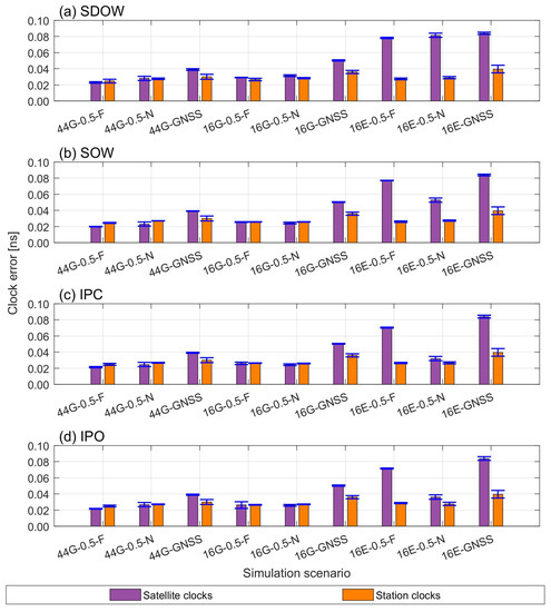
Figure 8.
Mean RMS estimation errors for satellite and station clocks considering the station set and VCE approach with respect to connectivity schemes: (a) sequential dial one-way (SDOW), (b) sequential one-way (SOW), (c) intra-plane closed (IPC), and (d) intra-plane open (IPO). The simulation scenario names are given in Table 7.
Figure 9 depicts values of SISRE(orb) and SISRE for adopted ground station sets and confirms that using ISL together with GNSS observations, even with a limited number of uniformly distributed ground stations, helps to improve position accuracy compared with the GNSS-only solution. In GNSS + ISL case, for the same ISL range bias value and with globally located stations mean SISRE(orb) is equal to 0.5 cm while mean SISRE to about 1.0 cm, regardless the connectivity schemes. When using a regional set of station results, SISRE values are characterized with very small repeatability in subsequent simulations, even with the support of ISLs. For simulation scenarios using 16 stations located in Europe, the connectivity scheme and geometrical properties can strongly impact the orbit accuracy. Thus, regional ground station sets are not recommended for precise orbit determination when it is possible to use globally located ground stations, even when ISLs are available.
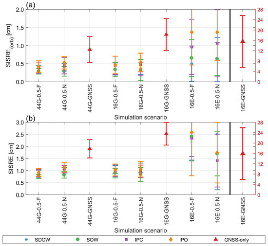
Figure 9.
(a) SISRE(orb) and (b) SISRE values computed under different simulation scenarios. Please note that values for 16E-GNSS are presented with different vertical axis in cm.
4. Discussion and Conclusions
This research aimed to consider the use of relative weighting in combined orbit determination when two or more observation techniques are used. We performed simulations with various input parameters to deeply investigate the impact of used VCE approaches when different ISL range biases are present and distinct ground station sets are used.
Using the Helmert or Förstner approach of the VCE method may be beneficial in future processing schemes exploiting ISLs and GNSS measurements in the Galileo system. In Zhang et al. [15], the VCE algorithm was already applied to the parameter estimation of the satellite orbit determination in BeiDou with ISLs. The results in Zhang et al. [15] confirm that orbit accuracy was improved after the adjustment of the VCE algorithm in the fusion data processing including 10 ground stations located in China in addition to ISLs. For different processing settings (e.g., constellation, station placement, and errors), the general conclusions about the VCE exploitation also reveal that the orbit determination accuracy is improved.
An initial check of possibility for ISL range bias estimation has been conducted in Kur et al. [34] and it was suggested that accurate ISL range bias estimation is possible because of the GNSS observations. In this research, we analyze 44 and 16 stations uniformly distributed around the world, and 16 stations located only in Europe to verify the impact of the number of ground stations and their placement on the VCE approaches and the ISL range bias estimation possibilities. In addition, estimation of ISL range biases was investigated in Michalak et al. [31] and it was shown that ISL range biases up to 5 mm have no significant impact on ISL residuals and clock estimation errors, but ISL range biases introduce a considerable error in the radial component. Michalak et al. [31] suggest implementing precise ground calibration of the instruments rather than estimation of range biases as estimated ISL range biases may deviate from the simulated values due to modelling errors. In contrast, in He et al. [17] it was suggested that calibration is not necessary as the estimation provides results with sufficient accuracy. However, it is worth paying attention to the simulation settings and estimation properties, which are distinct in these works. Still, the best-suited ISL range bias calibration remains uncertain as different analyses based on various simulation approaches or estimation settings provide incompatible results. This will be a challenge that is difficult to solve in simulations as the onboard hardware in orbit may face conditions that are considerably different from the current assumptions. Ground calibration of ISL range biases remains an open question that we would like to address in future analysis.
For the Galileo constellation, we can only test the hypothesis concerning ISL processing with the use of simulated measurements. Simulations are a great tool to check possible solutions, as we know exactly which effects were introduced. In this research on employing ISLs in Galileo, we tested three interlacing cases using relative weighting methods: (1) comparison under a strict (Helmert) and simplified approach (Förstner) to the VCE, (2) results of bias estimation in view of the weighting method, and (3) possible impact of the number of ground stations and their location on Earth.
Firstly, we found that the VCE helps to minimize errors for satellite positions without impacting clock estimation. However, the total gain is no more than 20% compared with the Nominal weighting method when the least optimal simulation scenario was used. Förstner and Helmert approaches to the VCE perform similarly. The Helmert approach is considered here as a strict solution with higher computational burden than the Förstner approach because of the necessity for least-squares adjustment of weighting coefficients rather than a straightforward formula.
Secondly, we demonstrate ISL range bias estimation considering weighting method, number, and location of ground stations, but also the value of the ISL range bias. The results indicate that in applied settings, the number of stations is not critical in achieving a good accuracy of bias estimation (differences are usually <±25% of applied value). The differences between simulated and estimated bias are lower when VCE is used. This is especially clear for intra-plane schemes for which the observation geometry is insufficiently variable. Static connectivity schemes (i.e., intra-plane schemes) used in estimation without VCE has about 2–3 times greater differences from the simulated constant value.
Finally, we focused on the impact of ground station sets on ISL range bias estimation and overall orbit determination accuracy to complete the research. These results agree with our previous analysis in terms of exploited number of stations with using ISL measurements in orbit determination but without using VCE as the primary weighting method [12,34]. In the case of number and distribution of the stations, the number of GNSS measurements plays a vital role while exploiting the VCE. The RMS orbit errors show the possible improvement with the Förstner approach when the station distribution is poor compared to the Nominal weighting. The ISLs might have a larger impact on accuracy when the uniform station location cannot be used. In this case the use of VCE is the most justified to obtain better accuracy. For clock estimation, the choice of weighting methods is not as crucial as station distribution (as a consequence of the number of GNSS measurements) and contribution of ISLs.
In general, the choice of the connectivity schemes is essential in the presented ISL simulations. Schemes created according to constellation geometry properties or routing schemes created in advance might be succeeded by schemes created by more sophisticated algorithms to optimize data transfer but require broadcast orbits. Thus, further investigation of this topic will be important in future ISL development.
In conclusion, the relative weighting might be an additional value to include in processing schemes in orbit determination based on ISL and GNSS measurements. Here, we focused on relative weighting of measurements from two technologies to assess their impact on the combined solution. The results indicate the usefulness of VCE for orbit determination when ISL range bias estimation is assumed as a constant value per day per satellite. These findings may be helpful for future practical application in orbit determination with ISLs use. However, further research on ISL range biases and their calibration and further estimation possibilities should be conducted.
Author Contributions
Conceptualization, T.K. and T.L.; methodology, T.K. and T.L.; validation, T.K. and T.L.; investigation, T.K.; writing—original draft preparation, T.K.; writing—review and editing, T.L.; visualization, T.K. All authors have read and agreed to the published version of the manuscript.
Funding
This research received no external funding.
Institutional Review Board Statement
Not applicable.
Informed Consent Statement
Not applicable.
Data Availability Statement
Not applicable.
Acknowledgments
Authors would like to sincerely thank Maciej Kalarus for discussions, relevant suggestions, and constructive comments that helped in improving this paper.
Conflicts of Interest
The authors declare no conflict of interest.
Appendix A

Figure A1.
Mean estimated ISL range biases of each satellite (simulated value of 0.5 cm) for different ground station sets: (a) 44 stations (global), (b) 16 stations (global), and (c) 16 stations (Europe) under different weighting methods.
Figure A1.
Mean estimated ISL range biases of each satellite (simulated value of 0.5 cm) for different ground station sets: (a) 44 stations (global), (b) 16 stations (global), and (c) 16 stations (Europe) under different weighting methods.


Figure A2.
Impact of ground station set on orbit estimation mean RMS errors for (a) radial, (b) along-track, (c) cross-track components, and (d) the total 3D RMS value. Description of simulation scenario names are given in Table 7. Please note the different y-axis scale for the regional station set and the GNSS-only solution. The results in cm for GNSS-only are on the vertical axis on the right marked in red.

References
- Sun, L.; Huang, W.; Gao, S.; Li, W.; Guo, X.; Yang, J. Joint Timekeeping of Navigation Satellite Constellation with Inter-Satellite Links. Sensors 2020, 20, 670. [Google Scholar] [CrossRef]
- Ruan, R.; Jia, X.; Feng, L.; Zhu, J.; Huyan, Z.; Li, J.; Wei, Z. Orbit Determination and Time Synchronization for BDS-3 Satellites with Raw Inter-Satellite Link Ranging Observations. Satell. Navig. 2020, 1, 8. [Google Scholar] [CrossRef]
- Fernández, F.A. Inter-Satellite Ranging and Inter-Satellite Communication Links for Enhancing GNSS Satellite Broadcast Navigation Data. Adv. Space Res. 2011, 47, 786–801. [Google Scholar] [CrossRef]
- Guo, L.; Wang, F.; Gong, X.; Sang, J.; Liu, W.; Zhang, W. Initial Results of Distributed Autonomous Orbit Determination for Beidou BDS-3 Satellites Based on Inter-Satellite Link Measurements. GPS Solut. 2020, 24, 72. [Google Scholar] [CrossRef]
- Tang, C.; Hu, X.; Zhou, S.; Liu, L.; Pan, J.; Chen, L.; Guo, R.; Zhu, L.; Hu, G.; Li, X.; et al. Initial Results of Centralized Autonomous Orbit Determination of the New-Generation BDS Satellites with Inter-Satellite Link Measurements. J. Geod. 2018, 92, 1155–1169. [Google Scholar] [CrossRef]
- Pan, J.; Hu, X.; Zhou, S.; Tang, C.; Wang, D.; Yang, Y.; Dong, W. Full-ISL Clock Offset Estimation and Prediction Algorithm for BDS3. GPS Solut. 2021, 25, 140. [Google Scholar] [CrossRef]
- Yang, D.; Yang, J.; Xu, P. Timeslot Scheduling of Inter-Satellite Links Based on a System of a Narrow Beam with Time Division. GPS Solut. 2017, 21, 999–1011. [Google Scholar] [CrossRef]
- Sun, L.; Yang, J.; Huang, W.; Xu, L.; Cao, S.; Shao, H. Inter-Satellite Time Synchronization and Ranging Link Assignment for Autonomous Navigation Satellite Constellations. Adv. Space Res. 2022, 69, 2421–2432. [Google Scholar] [CrossRef]
- Zhou, W.; Gao, W.; Lin, X.; Hu, X.; Ren, Q.; Tang, C. Emerging Errors in the Orientation of the Constellation in GNSS Autonomous Orbit Determination Based on Inter-Satellite Link Measurements. Adv. Space Res. 2022, 70, 3156–3172. [Google Scholar] [CrossRef]
- Gong, X.; Huang, D.; Cai, S.; Zhou, L.; Yuan, L.; Feng, W. Parameter Decomposition Filter of BDS-3 Combined Orbit Determination Using Inter-Satellite Link Observations. Adv. Space Res. 2019, 64, 88–103. [Google Scholar] [CrossRef]
- Rodríguez-Pérez, I.; García-Serrano, C.; Catalán Catalán, C.; García, A.M.; Tavella, P.; Galleani, L.; Amarillo, F. Inter-Satellite Links for Satellite Autonomous Integrity Monitoring. Adv. Space Res. 2011, 47, 197–212. [Google Scholar] [CrossRef]
- Kur, T.; Kalarus, M. Simulation of Inter-Satellite Link Schemes for Use in Precise Orbit Determination and Clock Estimation. Adv. Space Res. 2021, 68, 4734–4752. [Google Scholar] [CrossRef]
- Yang, Y.; Yang, Y.; Guo, R.; Tang, C.; Zhang, Z. The Influence of Station Distribution on the BeiDou-3 Inter-Satellite Link Enhanced Orbit Determination. In China Satellite Navigation Conference (CSNC) 2020 Proceedings: Volume II. CSNC 2020; Sun, J., Yang, C., Xie, J., Eds.; Lecture Notes in Electrical Engineering; Springer: Singapore, 2020; Volume 651, pp. 58–70. [Google Scholar]
- Zhang, R.; Zhang, Q.; Huang, G.; Wang, L.; Qu, W. Impact of Tracking Station Distribution Structure on BeiDou Satellite Orbit Determination. Adv. Space Res. 2015, 56, 2177–2187. [Google Scholar] [CrossRef]
- Zhang, R.; Tu, R.; Zhang, P.; Fan, L.; Han, J.; Lu, X. Orbit Determination of BDS-3 Satellite Based on Regional Ground Tracking Station and Inter-Satellite Link Observations. Adv. Space Res. 2021, 67, 4011–4024. [Google Scholar] [CrossRef]
- Zhang, R.; Tu, R.; Zhang, P.; Fan, L.; Han, J.; Wang, S.; Hong, J.; Lu, X. Optimization of Ground Tracking Stations for BDS-3 Satellite Orbit Determination. Adv. Space Res. 2021, 68, 4069–4087. [Google Scholar] [CrossRef]
- He, X.; Hugentobler, U.; Schlicht, A.; Nie, Y.; Duan, B. Precise Orbit Determination for a Large LEO Constellation with Inter-Satellite Links and the Measurements from Different Ground Networks: A Simulation Study. Satell. Navig. 2022, 3, 22. [Google Scholar] [CrossRef]
- Zhang, R.; Tu, R.; Fan, L.; Zhang, P.; Liu, J.; Han, J.; Lu, X. Contribution Analysis of Inter-Satellite Ranging Observation to BDS-2 Satellite Orbit Determination Based on Regional Tracking Stations. Acta Astronaut. 2019, 164, 297–310. [Google Scholar] [CrossRef]
- Yang, Y.; Yang, Y.; Hu, X.; Tang, C.; Guo, R.; Zhou, Z.; Xu, J.; Pan, J.; Su, M. BeiDou-3 Broadcast Clock Estimation by Integration of Observations of Regional Tracking Stations and Inter-Satellite Links. GPS Solut. 2021, 25, 57. [Google Scholar] [CrossRef]
- Li, X.; Hu, X.; Guo, R.; Tang, C.; Liu, S.; Xin, J.; Guo, J.; Tian, Y.; Yang, Y.; Yang, J.; et al. Precise Orbit Determination for BDS-3 GEO Satellites Enhanced by Intersatellite Links. GPS Solut. 2023, 27, 8. [Google Scholar] [CrossRef]
- Xie, X.; Geng, T.; Zhao, Q.; Liu, J.; Wang, B. Performance of BDS-3: Measurement Quality Analysis, Precise Orbit and Clock Determination. Sensors 2017, 17, 1233. [Google Scholar] [CrossRef]
- Xie, X.; Geng, T.; Zhao, Q.; Cai, H.; Zhang, F.; Wang, X.; Meng, Y. Precise Orbit Determination for BDS-3 Satellites Using Satellite-Ground and Inter-Satellite Link Observations. GPS Solut. 2019, 23, 40. [Google Scholar] [CrossRef]
- Shi, J.; Ouyang, C.; Huang, Y.; Peng, W. Assessment of BDS-3 Global Positioning Service: Ephemeris, SPP, PPP, RTK, and New Signal. GPS Solut. 2020, 24, 81. [Google Scholar] [CrossRef]
- Zhu, Y.; Zhang, Q.; Mao, Y.; Cui, X.; Cai, C.; Zhang, R. Comprehensive Performance Review of BDS-3 after One-Year Official Operation. Adv. Space Res. 2022, in press. [CrossRef]
- Ren, X.; Yang, Y.; Zhu, J.; Xu, T. Comparing Satellite Orbit Determination by Batch Processing and Extended Kalman Filtering Using Inter-Satellite Link Measurements of the next-Generation BeiDou Satellites. GPS Solut. 2019, 23, 25. [Google Scholar] [CrossRef]
- Zhou, Y.; Wang, Y.; Huang, W.; Yang, J.; Sun, L. In-Orbit Performance Assessment of BeiDou Intersatellite Link Ranging. GPS Solut. 2018, 22, 119. [Google Scholar] [CrossRef]
- Pan, J.; Hu, X.; Zhou, S.; Tang, C.; Guo, R.; Zhu, L.; Tang, G.; Hu, G. Time Synchronization of New-Generation BDS Satellites Using Inter-Satellite Link Measurements. Adv. Space Res. 2018, 61, 145–153. [Google Scholar] [CrossRef]
- Xie, X.; Geng, T.; Zhao, Q.; Lv, Y.; Cai, H.; Liu, J. Orbit and Clock Analysis of BDS-3 Satellites Using Inter-Satellite Link Observations. J. Geod. 2020, 94, 64. [Google Scholar] [CrossRef]
- Tang, C.; Hu, X.; Zhou, S.; Guo, R.; He, F.; Liu, L.; Zhu, L.; Li, X.; Wu, S.; Zhao, G.; et al. Improvement of Orbit Determination Accuracy for Beidou Navigation Satellite System with Two-Way Satellite Time Frequency Transfer. Adv. Space Res. 2016, 58, 1390–1400. [Google Scholar] [CrossRef]
- An Official Website of the European Union. Available online: https://defence-industry-space.ec.europa.eu/commission-awards-eu147-bn-contracts-launch-2nd-generation-galileo-satellites-2021-01-20_en (accessed on 22 November 2022).
- Michalak, G.; Glaser, S.; Neumayer, K.H.; König, R. Precise Orbit and Earth Parameter Determination Supported by LEO Satellites, Inter-Satellite Links and Synchronized Clocks of a Future GNSS. Adv. Space Res. 2021, 68, 4753–4782. [Google Scholar] [CrossRef]
- Marz, S.; Schlicht, A.; Hugentobler, U. Galileo Precise Orbit Determination with Optical Two-Way Links (OTWL): A Continuous Wave Laser Ranging and Time Transfer Concept. J. Geod. 2021, 95, 85. [Google Scholar] [CrossRef]
- Schlicht, A.; Marz, S.; Stetter, M.; Hugentobler, U.; Schäfer, W. Galileo POD Using Optical Inter-Satellite Links: A Simulation Study. Adv. Space Res. 2020, 66, 1558–1570. [Google Scholar] [CrossRef]
- Kur, T.; Liwosz, T.; Kalarus, M. The Application of Inter-Satellite Links Connectivity Schemes in Various Satellite Navigation Systems for Orbit and Clock Corrections Determination: Simulation Study. Acta Geod. Geophys. 2021, 56, 1–28. [Google Scholar] [CrossRef]
- Glaser, S.; Michalak, G.; Konig, R.; Mannel, B.; Schuh, H. Future GNSS Infrastructure for Improved Geodetic Reference Frames. In Proceedings of the 2020 European Navigation Conference (ENC), Dresden, Germany, 23–24 November 2020; IEEE: Piscataway, NJ, USA, 2020; pp. 1–10. [Google Scholar]
- Yang, D.; Yang, J.; Li, G.; Zhou, Y.; Tang, C.P. Globalization Highlight: Orbit Determination Using BeiDou Inter-Satellite Ranging Measurements. GPS Solut. 2017, 21, 1395–1404. [Google Scholar] [CrossRef]
- Guo, R.; Hu, X.G.; Tang, B.; Huang, Y.; Liu, L.; Cheng, L.C.; He, F. Precise Orbit Determination for Geostationary Satellites with Multiple Tracking Techniques. Chin. Sci. Bull. 2010, 55, 687–692. [Google Scholar] [CrossRef]
- Liu, L.; Zhu, L.F.; Han, C.H.; Liu, X.P.; Li, C. The Model of Radio Two-Way Time Comparison between Satellite and Station and Experimental Analysis. Chin. Astron. Astrophys. 2009, 33, 431–439. [Google Scholar] [CrossRef]
- Shi, L.Y.; Xiang, W.; Tang, X.M. A Link Assignment Algorithm for GNSS with Crosslink Ranging. In Proceedings of the 2011 International Conference on Localization and GNSS, ICL-GNSS 2011, Tampere, Finland, 29–30 June 2011; pp. 13–18. [Google Scholar]
- Xu, B.; Han, K.; Ren, Q.; Gong, W.; Shao, F.; Wang, Y.; Chang, J. An Optimized Strategy for Inter-Satellite Links Assignments in GNSS. Adv. Space Res. 2022, in press. [CrossRef]
- Han, S.; Gui, Q.; Li, J. Establishment Criteria, Routing Algorithms and Probability of Use of Inter-Satellite Links in Mixed Navigation Constellations. Adv. Space Res. 2013, 51, 2084–2092. [Google Scholar] [CrossRef]
- Werner, M.; Delucchi, C.; Vögel, H.J.; Maral, G.; de Ridder, J.J. ATM-Based Routing in LEO/MEO Satellite Networks with Intersatellite Links. IEEE J. Sel. Areas Commun. 1997, 15, 69–82. [Google Scholar] [CrossRef]
- Yi, X.; Sun, Z.; Yao, F.; Miao, Y. Satellite Constellation of MEO and IGSO Network Routing with Dynamic Grouping. Int. J. Satell. Commun. Netw. 2013, 31, 277–302. [Google Scholar] [CrossRef]
- Huang, J.; Su, Y.; Liu, W.; Wang, F. Optimization Design of Inter-Satellite Link (ISL) Assignment Parameters in GNSS Based on Genetic Algorithm. Adv. Space Res. 2017, 60, 2574–2580. [Google Scholar] [CrossRef]
- Sun, L.; Wang, Y.; Huang, W.; Yang, J.; Zhou, Y.; Yang, D. Inter-Satellite Communication and Ranging Link Assignment for Navigation Satellite Systems. GPS Solut. 2018, 22, 38. [Google Scholar] [CrossRef]
- Huang, J.; Liu, W.; Su, Y.; Wang, F. Cascade Optimization Design of Inter-Satellite Link Enhanced with Adaptability in Future GNSS Satellite Networks. GPS Solut. 2018, 22, 44. [Google Scholar] [CrossRef]
- Yan, J.; Xing, L.; Wang, P.; Sun, L.; Chen, Y. A Scheduling Strategy to Inter-Satellite Links Assignment in GNSS. Adv. Space Res. 2021, 67, 198–208. [Google Scholar] [CrossRef]
- Zeng, L.; Lu, X.; Bai, Y.; Liu, B.; Yang, G. Topology Design Algorithm for Optical Inter-Satellite Links in Future Navigation Satellite Networks. GPS Solut. 2022, 26, 57. [Google Scholar] [CrossRef]
- Han, S.; Gui, Q.; Li, G.; Du, Y. Minimum of PDOP and Its Applications in Inter-Satellite Links (ISL) Establishment of Walker-δ Constellation. Adv. Space Res. 2014, 54, 726–733. [Google Scholar] [CrossRef]
- Tang, Y.; Wang, Y.; Chen, J. The Availability of Space Service for Inter-Satellite Links in Navigation Constellations. Sensors 2016, 16, 1327. [Google Scholar] [CrossRef]
- Xu, H.; Wang, J.; Zhan, X. Autonomous Broadcast Ephemeris Improvement for GNSS Using Inter-Satellite Ranging Measurements. Adv. Space Res. 2012, 49, 1034–1044. [Google Scholar] [CrossRef]
- Senior, K.L.; Ray, J.R.; Beard, R.L. Characterization of Periodic Variations in the GPS Satellite Clocks. GPS Solut. 2008, 12, 211–225. [Google Scholar] [CrossRef]
- Pavlis, N.K.; Holmes, S.A.; Kenyon, S.C.; Factor, J.K. The Development and Evaluation of the Earth Gravitational Model 2008 (EGM2008). J. Geophys. Res. Solid Earth 2012, 117, 1–38. [Google Scholar] [CrossRef]
- Petit, G.; Luzum, B. (Eds.) IERS Conventions (2010); Federal Agency for Cartography and Geodesy: Frankfurt am Main, Germany, 2010; ISBN 3-89888-989-6.
- Galileo Satellite Metadata European Union Agency for the Space Programme. Available online: https://www.gsc-europa.eu/support-to-developers/galileo-satellite-metadata (accessed on 22 November 2022).
- Arnold, D.; Meindl, M.; Beutler, G.; Dach, R.; Schaer, S.; Lutz, S.; Prange, L.; Sośnica, K.; Mervart, L.; Jäggi, A. CODE’s New Solar Radiation Pressure Model for GNSS Orbit Determination. J. Geod. 2015, 89, 775–791. [Google Scholar] [CrossRef]
- Zehentner, N. Kinematic Orbit Positioning Applying the Raw Observation Approach to Observe Time Variable Gravity. Ph.D. Thesis, Graz University of Technology, Graz, Austria, 2016. [Google Scholar] [CrossRef]
- Teunissen, P.J.G.; Amiri-Simkooei, A.R. Least-Squares Variance Component Estimation. J. Geod. 2008, 82, 65–82. [Google Scholar] [CrossRef]
- Zehentner, N.; Mayer-Gürr, T. Precise Orbit Determination Based on Raw GPS Measurements. J. Geod. 2016, 90, 275–286. [Google Scholar] [CrossRef]
- Kusche, J. Noise Variance Estimation and Optimal Weight Determination for GOCE Gravity Recovery. Adv. Geosci. 2003, 1, 81–85. [Google Scholar] [CrossRef]
- Wang, J.-G.; Gopaul, N.; Scherzinger, B. Simplified Algorithms of Variance Component Estimation for Static and Kinematic GPS Single Point Positioning. J. Glob. Position. Syst. 2009, 8, 43–52. [Google Scholar] [CrossRef]
- Li, M.; Nie, W.; Xu, T.; Rovira-Garcia, A.; Fang, Z.; Xu, G. Helmert Variance Component Estimation for Multi GNSS Relative Positioning. Sensors 2020, 20, 669. [Google Scholar] [CrossRef] [PubMed]
- Zangeneh-Nejad, F.; Amiri-Simkooei, A.R.; Sharifi, M.A.; Asgari, J. Recursive Least Squares with Real Time Stochastic Modeling: Application to GPS Relative Positioning. In Proceedings of the International Archives of the Photogrammetry, Remote Sensing and Spatial Information Sciences—ISPRS Archives, International Society for Photogrammetry and Remote Sensing: 2017 Tehran’s Joint ISPRS Conferences of GI Research, SMPR and EOEC 2017, Tehran, Iran, 7–10 October 2017; Volume 42, pp. 531–536. [Google Scholar]
- Bähr, H.; Altamimi, Z.; Heck, B. Variance Component Estimation for Combination of Terrestrial Reference Frames; Schriftenreihe des Studiengangs Geodäsie und Geoinformatik, Studiengang Geodäsie und Geoinformatik; Universität Karlsruhe (TH): Karlsruhe, Germany, 2007. [Google Scholar]
- Amiri-Simkooei, A.R. Parameter Estimation in 3D Affine and Similarity Transformation: Implementation of Variance Component Estimation. J. Geod. 2018, 92, 1285–1297. [Google Scholar] [CrossRef]
- Xu, T.; Xue, T.; Xu, G.; Shen, X.; Shan, X.; Chen, Y. A Maneuvered GEO Satellite Orbit Determination Using Robustly Adaptive Kalman Filter. In Proceedings of the 2010 International Conference on Intelligent System Design and Engineering Application, ISDEA 2010, Changsha, China, 13–14 October 2010; IEEE Computer Society: Piscataway, NJ, USA, 2010; Volume 1, pp. 55–59. [Google Scholar]
- Amiri-Simkooei, A.R. Least-Squares Variance Component Estimation: Theory and GPS Applications. Ph.D. Thesis, Delft University of Technology, Delft, The Netherlands, 2007. [Google Scholar]
- Hauschild, A.; Montenbruck, O. Kalman-Filter-Based GPS Clock Estimation for near Real-Time Positioning. GPS Solut. 2009, 13, 173–182. [Google Scholar] [CrossRef]
- Montenbruck, O.; Steigenberger, P.; Hauschild, A. Broadcast versus Precise Ephemerides: A Multi-GNSS Perspective. GPS Solut. 2015, 19, 321–333. [Google Scholar] [CrossRef]
- Steigenberger, P.; Montenbruck, O. Galileo Status: Orbits, Clocks, and Positioning. GPS Solut. 2017, 21, 319–331. [Google Scholar] [CrossRef]


Publisher’s Note: MDPI stays neutral with regard to jurisdictional claims in published maps and institutional affiliations. |
© 2022 by the authors. Licensee MDPI, Basel, Switzerland. This article is an open access article distributed under the terms and conditions of the Creative Commons Attribution (CC BY) license (https://creativecommons.org/licenses/by/4.0/).