1. Introduction
Crop production is the cornerstone of social development. According to the Statistical Yearbook 2021 of the Food and Agriculture Organization of the United Nations, about 1.6 billion ha of global croplands provided all cereals, vegetables, fruits, and other crop products to support peoples’ lives [
1]. Such large-scale crop production and important food-security issues pose serious challenges to the precise management of crop cultivation. Remote sensing technology has become an effective means to provide accurate and low-cost services for crop cultivation [
2,
3,
4,
5], including early warning of pests and diseases [
6,
7], monitoring of nutrient and phenological phases [
8,
9], and irrigation–water estimations [
10,
11], etc. Spatial information on crop distribution is a prerequisite for specific analysis using remote sensing.
There are two main strategies for crop identification via remote sensing technology [
12]. The first strategy considers the spectral characteristics of a single remote sensing image captured at a certain time; however, the optimal date can hardly be determined because crop fields exhibit similar spectral characteristics to those of other fields during the early and growing seasons [
12,
13]. The conspicuous phenomenon of different objects with the same spectral characteristics can produce more identification errors [
14,
15]. Therefore, the second strategy uses the spectral and temporal characteristics to characterize unique identification features including specific spectral values revealing phenological characteristics and the spectral variance reflecting growth variation [
16,
17,
18,
19]. For instance, Hu et al. [
16] identified maize by using the differences in vegetation index (VI) values between maize and other fields over time. Shahrabi et al. [
18] found that the temporal–spectral variance in the normalized difference vegetation index (NDVI) during the crop growing season could be used to compute an appropriate variable for maize identification.
The spectral similarity and difference metric (SSDM) is usually used to classify surface objects. This can characterize the interclass spectral separability or intraclass spectral variability [
20,
21,
22,
23]. There are four main SSDM computation methods: (1) the SSDM is computed based on the spectral distance, including the Euclidean distance algorithm (ED) [
20,
22] and the Jeffries–Matusita distance algorithm [
23,
24]; (2) the SSDM is computed using the spectral angle, including the spectral angle mapper algorithm (SAM) [
25,
26] and spectral gradient angle algorithm [
27]; (3) the SSDM is computed via spectral information metrics, including the spectral information divergence algorithm [
28]; and (4) the SSDM is computed considering the spectral correlation, including the spectral correlation measures algorithm [
29]. Methods (1) and (2) are commonly used to identify crops involving remote sensing data, which assumes that the spectral characteristics are vectors in high-dimensional space, the dimensionality matches the number of spectral characteristics, and that the vector elements are the reflectance or VI [
20,
22,
23]. Several researchers [
20,
21,
22,
23,
30,
31] directly computed the SSDM between a reference-class spectrum and other pixel spectra with different spatial locations using methods (1) and (2). According to the quantized values of SSDM, they mapped the large-scale spatial distribution of crops including maize, soybean, wheat, and paddy rice in China and the United States, utilizing a Moderate Resolution Imaging Spectroradiometer (MODIS) and Sentinel-1 and Sentinel-2 (S2) data. The above SSDM could be equivalent to the spectral variance associated with the spatial location. If two spectra of a single pixel on different dates were used for SSDM computation via methods (1) and (2), the obtained SSDM would be equivalent to the spectral variance associated with the time. As mentioned above, the temporal–spectral variance is helpful for crop identification [
17,
18], so we conjecture that the temporal–spectral variance computed via the SSDM computation methods has the same capability. However, there is little research that has validated this.
Our group intends to use ED and SAM for computing a new identification index; namely, the spectral variance at key stages (SVKS), in which the key stages cover phenological and land-use changes. Given that the computation processes of the ED and SAM are relatively uncomplicated, SVKS could become a type of universal and effective identification index similar to vegetation indexes for crop identification. Nevertheless, certain limitations of the ED and SAM cannot be neglected before application. The above temporal–spectral variance is directly related to the value of each element of the multidimensional vectors used in ED, while ED is insensitive to spectral shape variation [
28]. Even if the variation in the spectral shape could be described, two curves with similar shapes but greatly different amplitudes could not be accurately captured with SAM [
32]. Moreover, the reference curve selection and reconstruction problem cannot be ignored when using the algorithm to determine the spectral similarity and the difference between the target and reference [
21,
22]. Initially, a reference curve representing the entire class could be obtained by averaging multiple standard curves, resulting in a susceptibility of the reference curve to sequence shifts and dislocations, thus ultimately affecting the crop-identification accuracy [
20]. Furthermore, the intraclass spectral variability cannot be represented by the reference curve [
33] and researchers need to first determine the threshold range of each class [
21,
34]. Optimization methods for reference-curve reconstruction have been proposed [
30]; for example, Li et al. [
20], Shao et al. [
21], and Mondal et al. [
35] used the singular-value decomposition, Savitzky–Golay smoothing algorithm, asymmetric Gaussian smoothing algorithm, Fourier transformation and other methods for reference-curve reconstruction and found that spectral reconstruction could enhance the target identification accuracy. Nevertheless, the identification accuracy highly depends on the accuracy of the reconstructed reference curve.
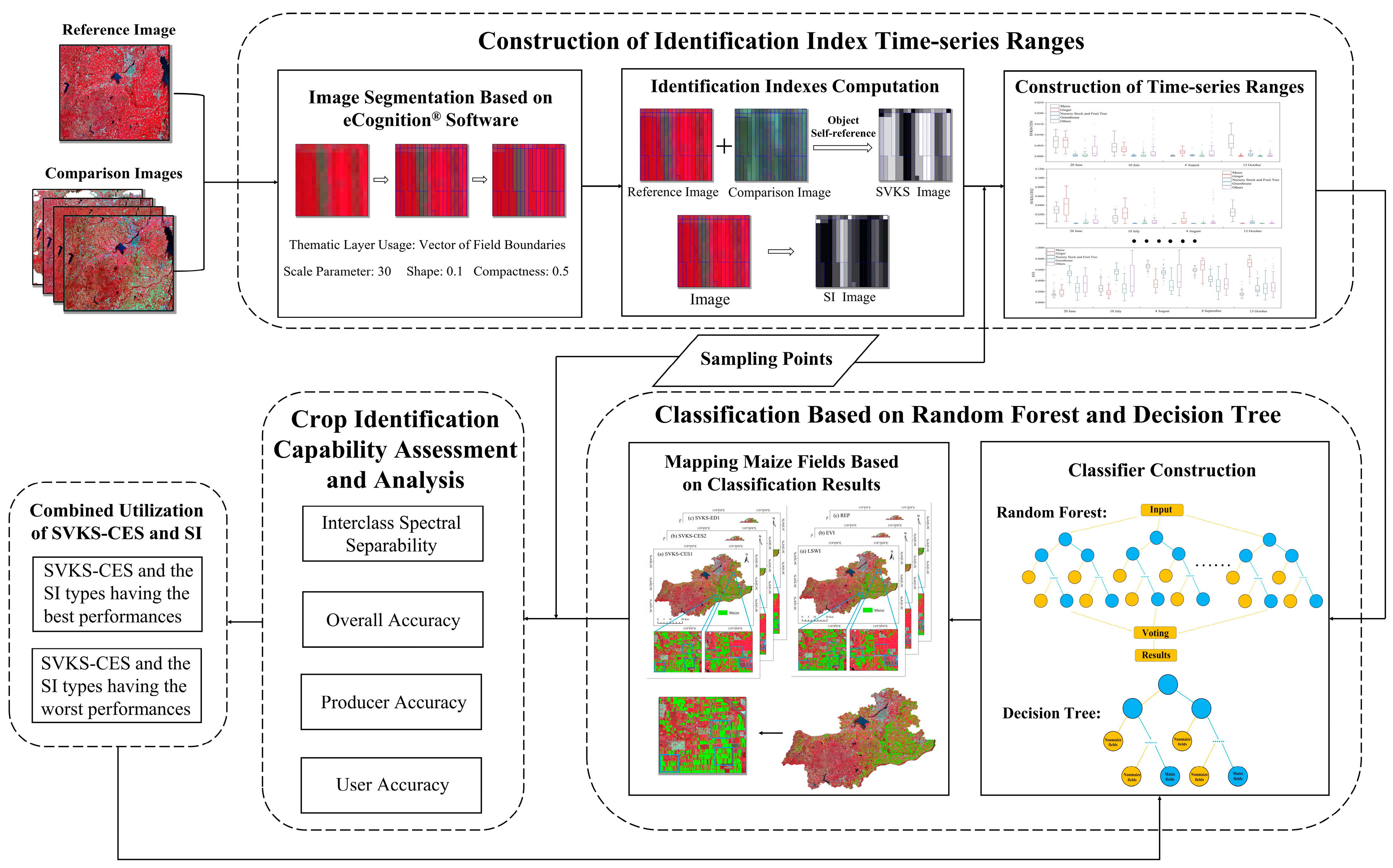
To integrate the sensibility advantages, a combined algorithm comprising ED and SAM (CES) was applied in SVKS calculation, which can eliminate the limitations of using ED or SAM alone. Furthermore, we proposed an object self-reference method for ED and SAM usage to avoid reconstructing a reference curve representing the entire class. Such improvements would universalize and simplify the calculation of SVKS; however, the crop identification potential for CES is unknown. Therefore, three contents were designed to validate the crop identification capability of SVKS-CES (SVKS computed via CES): (1) analyzing the SVKS-CES performances for characterizing interclass spectral separability; (2) selecting maize and non-maize as examples and comparing the maize-identification accuracy of SVKS-CES to SVKS-ED (SVKS computed via ED), SVKS-SAM (SVKS computed via SAM), and five spectral index (SI) types; and (3) applying combined utilization of SVKS-CES and SI for classification and assessing the capability of accuracy improvement.
4. Discussions
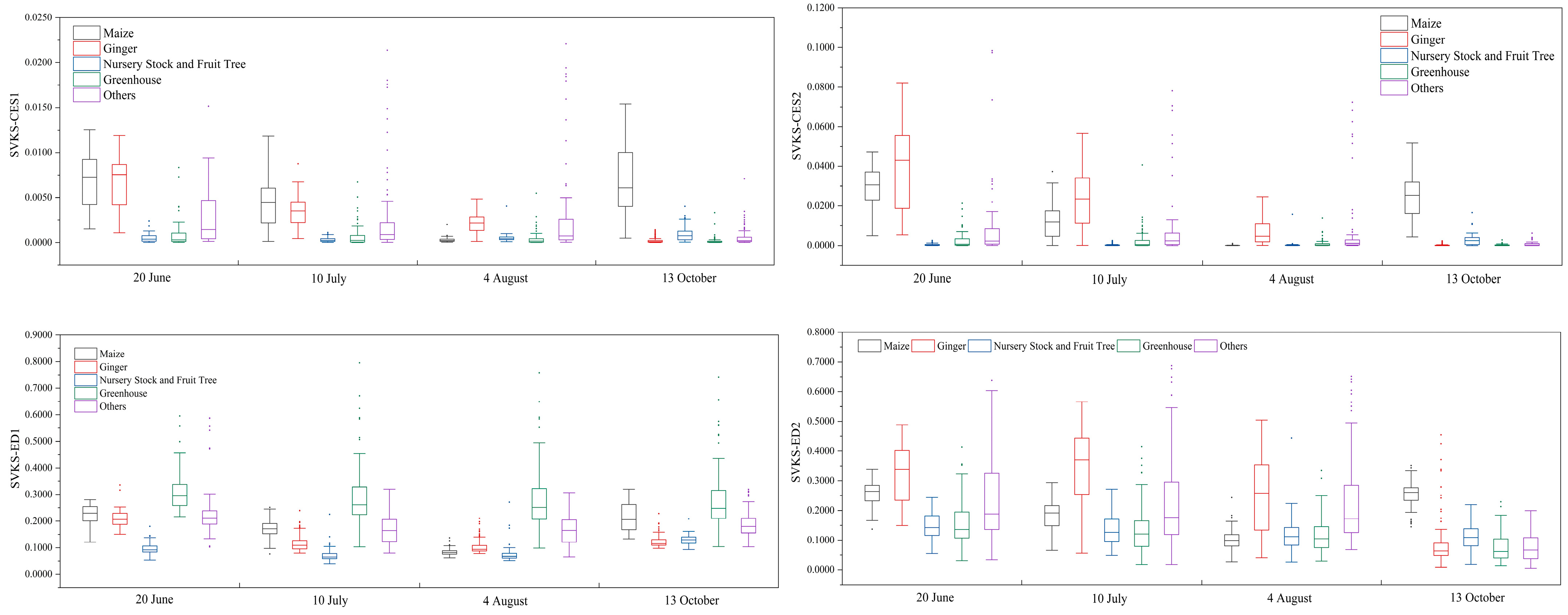
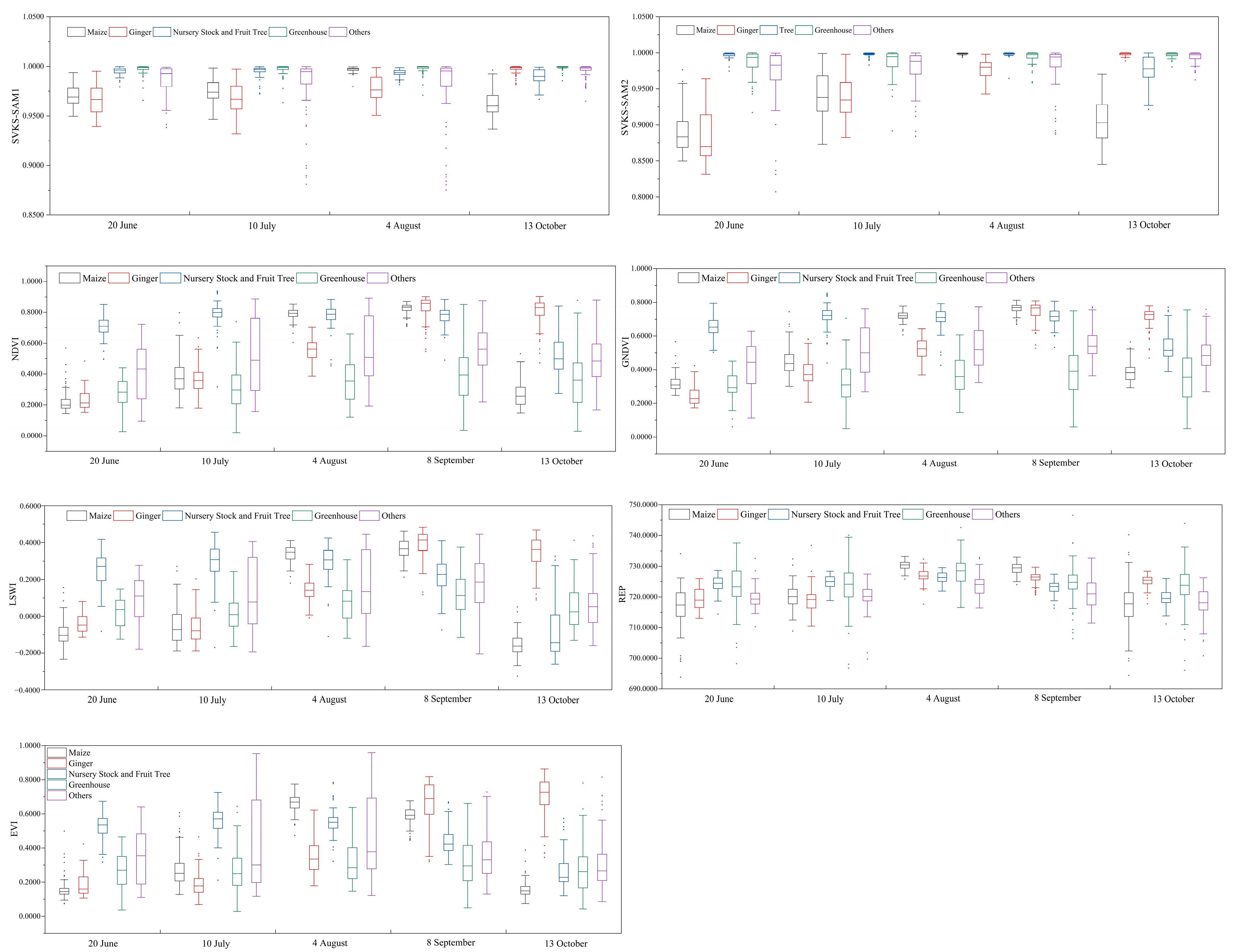
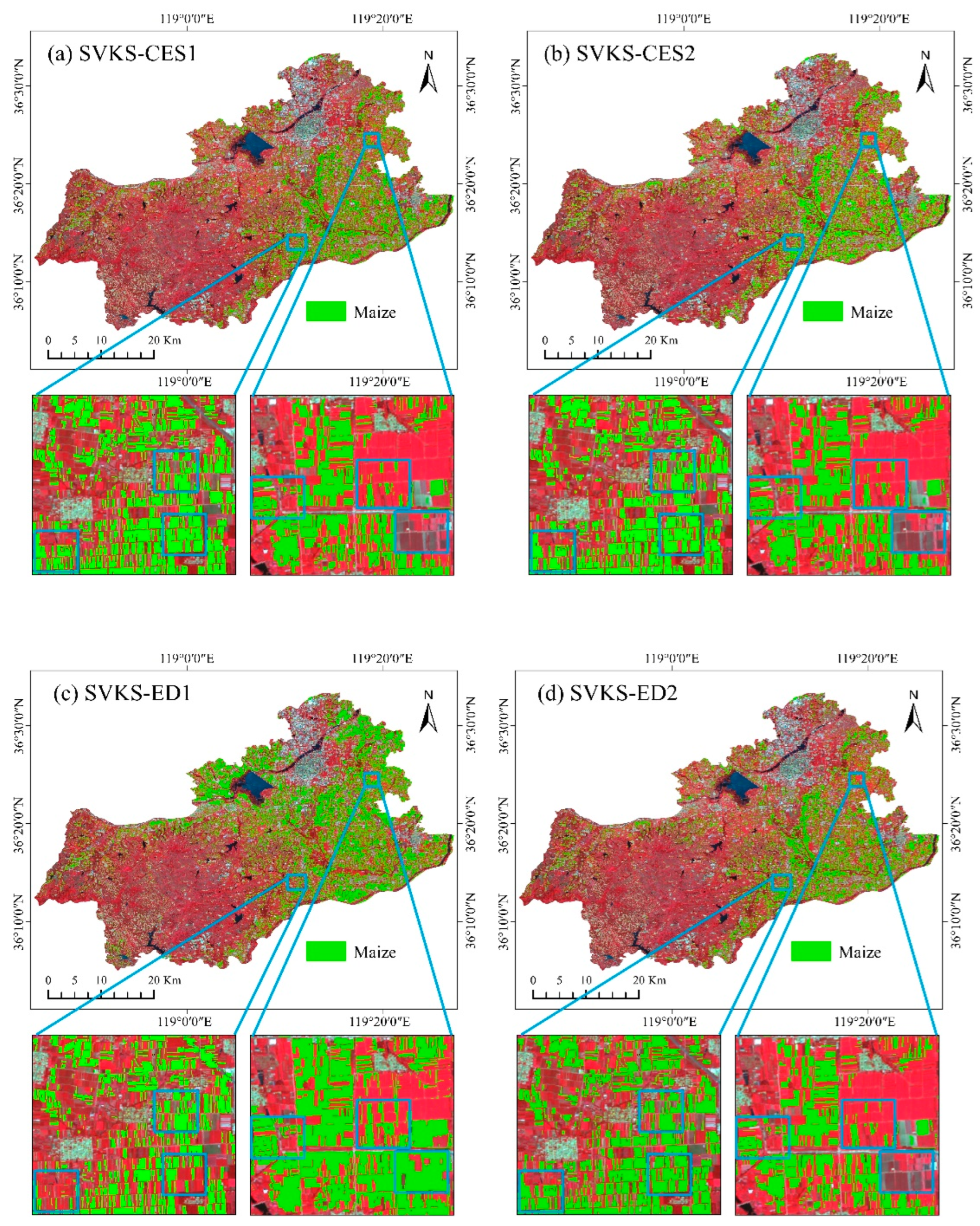
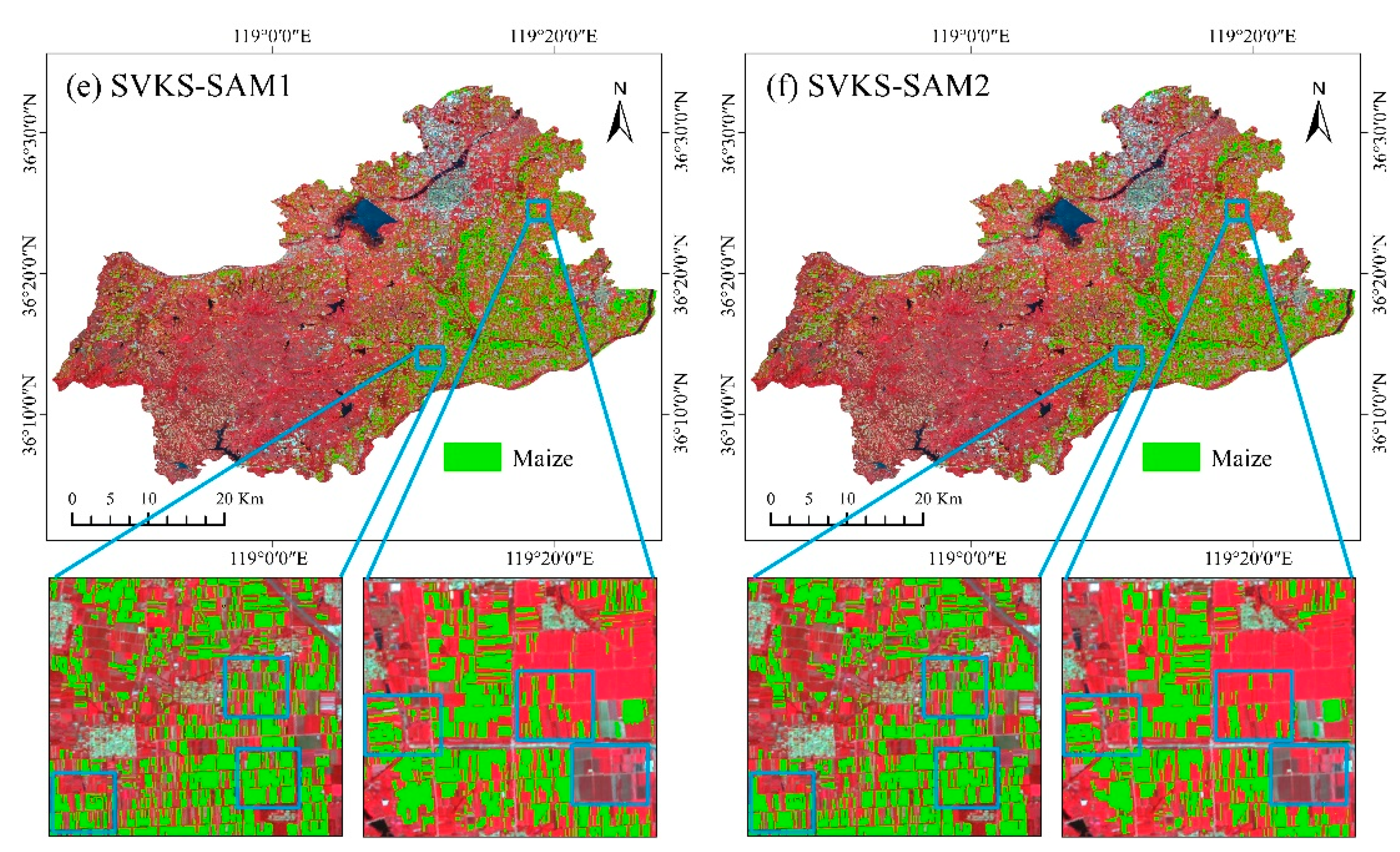
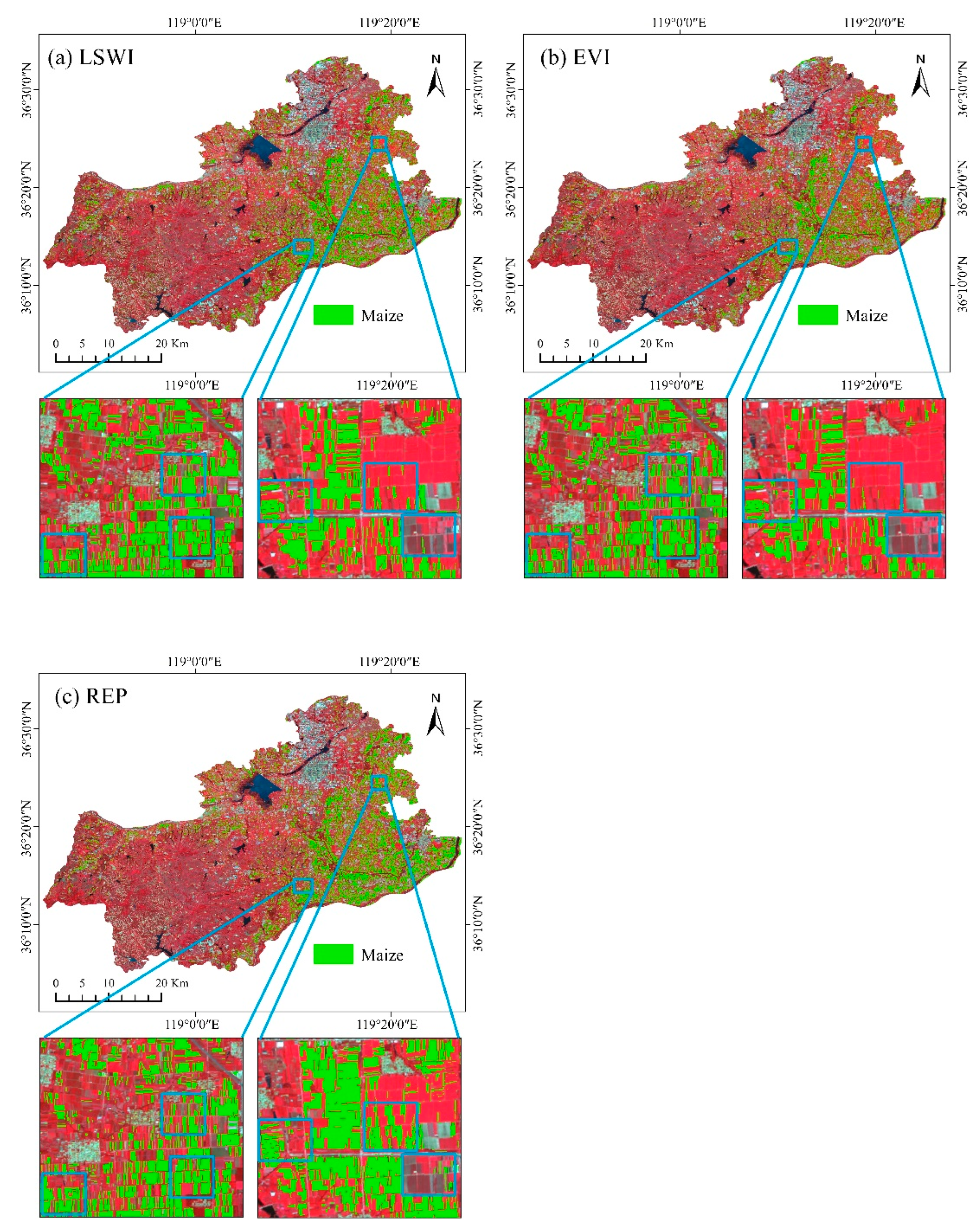
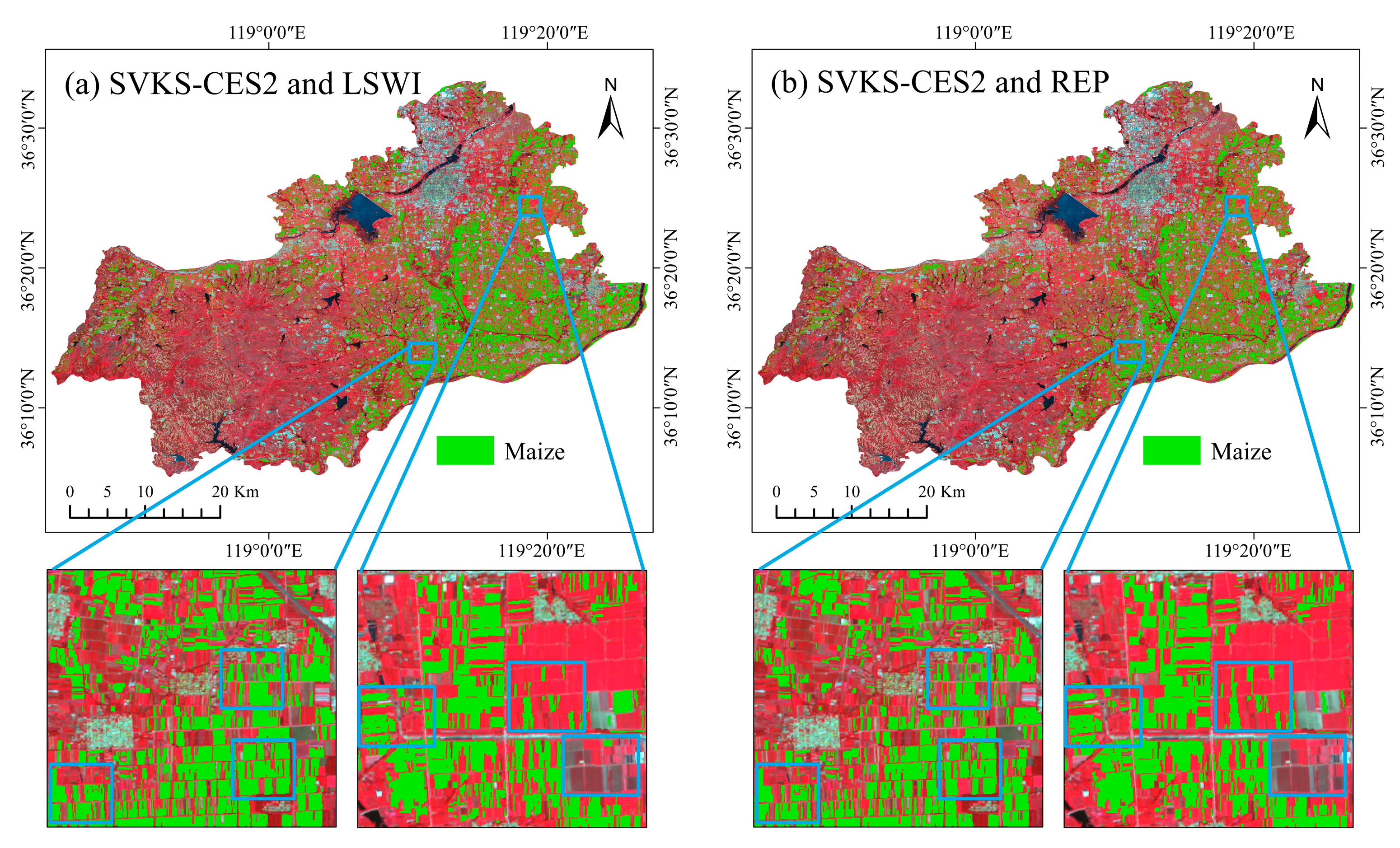
In this study, an object self-reference combined algorithm comprising ED and SAM (CES) was proposed to calculate SVKS and the crop-identification capability of SVKS-CES had been validated and discussed. Regarding the unique features characterized by the identification indexes, we found that SVKS-CES2 ranges of different classes had the least overlap compared to that of other identification indexes, which characterized that SVKS-CES2 ranges can provide the best interclass spectral separability. When selecting the feature for classifier training before classification, good interclass spectral separability is a useful indicator for determining which index has better crop-identification potential. For example, SVKS-CES2 and REP provide the best and worst interclass spectral separability and attained the best and worst identification accuracy, respectively. Regarding the SVKS performance in maize identification, the OA of SVKS-CES exceeded 96%, the PA of SVKS-CES exceeded 90%, and the UA exceeded 96%. Compared to the accuracy of other SVKS types, SVKS-CES exhibited the highest OA and UA which integrated the advantages of the highest PA of SVKS-ED and the higher UA of SVKS-SAM. The reason for these results could be that more key information benefiting identification is provided by the red-edge and NIR bands [
13,
44,
45]. It is helpful for SVKS to characterize the intraclass spectral variability and improve identification accuracy by increasing the number of bands in SVKS calculation. The number of bands could not exhibit the same increasing relationship as that of the SVKS accuracy as redundant bands could mask the distinction between classes and aggravate the typical phenomenon of different objects with the same spectral characteristics [
16,
46]. Compared to the accuracy of SVKS-CES2, SVKS-CES1 exhibited a lower PA, UA, and OA because the similar interclass spectral variance values attributed to similar visible-light absorption and chlorophyll-reflection levels could reduce the spectral separability between maize and non-maize fields [
12].
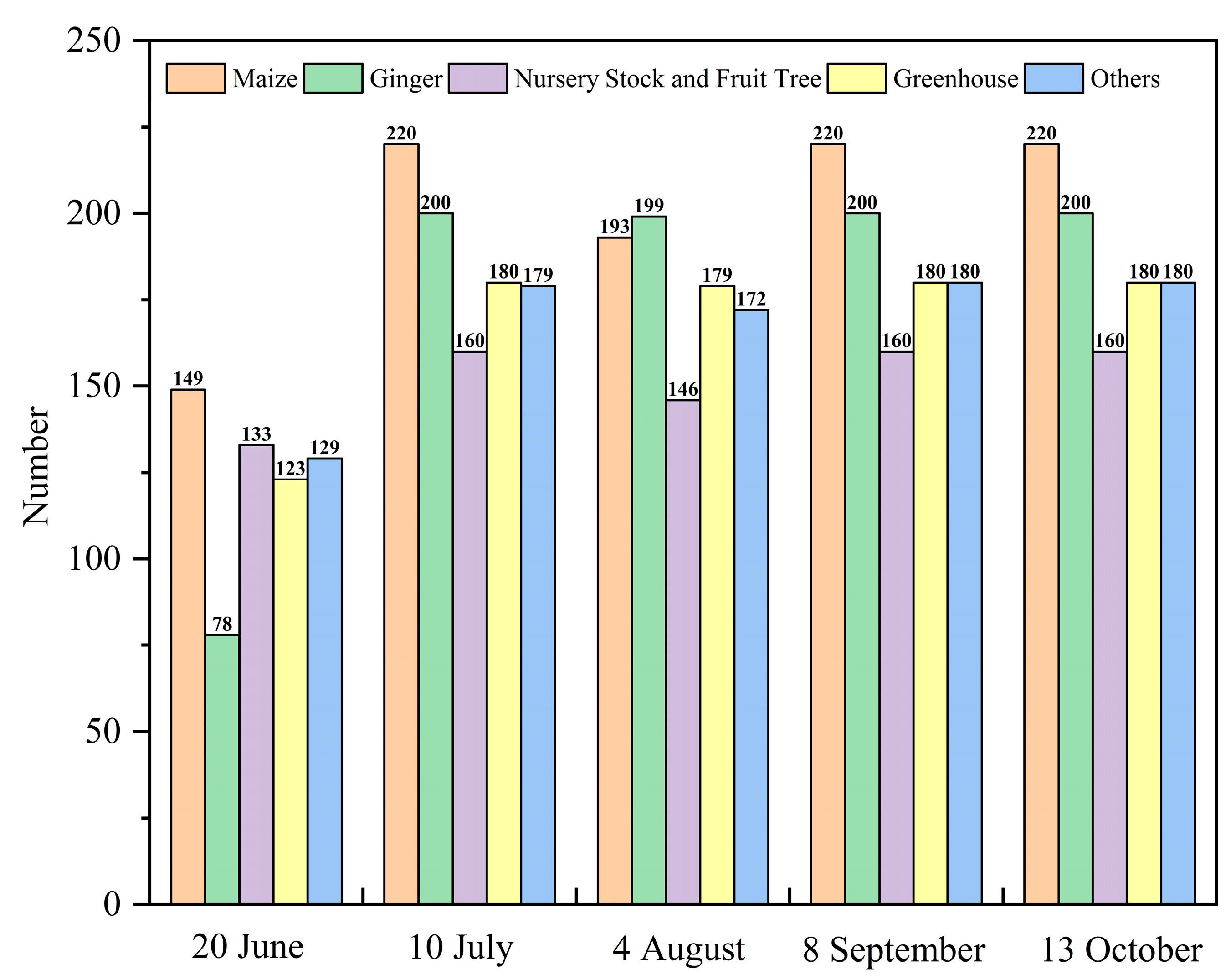
According to the temporal characteristics of SVKS, SVKS-CES could favorably distinguish maize from non-maize on 20 June and 13 October. We found that the SVKS-CES values of maize deviated from zero on 20 June, while those of nursery stock and fruit trees exhibited the opposite phenomenon as the spectrum curve of maize was similar to that of bare soil before the seedling stage but significantly different from that at the mature stage, while no considerable spectral variation occurred in nursery stock and fruit tree fields owing to the absence of senescence and harvesting. Furthermore, the SVKS-CES values of maize deviated from zero on 13 October while those of ginger, greenhouse, and others exhibited the opposite phenomenon due to the spectrum curve of maize being similar to that of bare soil or maize straw after the harvest. No considerable variation in the spectrum curve occurred in the ginger, greenhouse, and other fields owing to the absence of sowing or harvesting.
Compared to the performance of SI (the average PA, UA, and OA were 79.73%, 91.23% and 93.15%, respectively), we found that the average PA (89.39%) and OA (93.94) of SVKS were higher because of the better interclass spectral separability that occurred in SVKS ranges. However, more non-maize fields were incorrectly identified as maize fields using SVKS (the average UA was 88.94%), which indicates that interclass spectral variance similarity produced larger commission errors. The different performance levels of the various SI types indicated a great variation in identification results. Therefore, higher accuracy can be obtained by combining SVKS and certain SI types in maize identification [
12]. To assess the capability of accuracy improvement, SVKS-CES2 was selected to be combined with LSWI and REP for classification. The results showed that the addition of SVKS-CES2 can obviously reduce the omission and commission errors from LSWI- or REP-based classification, which illustrated that SVKS-CES provides greater application potential in crop identification. This is a promotion for feature selection before classifier training. We also applied various SVKS-CES and SI combinations to identify
glycyrrhiza uralensis Fisch. plants and achieved satisfactory results.
The following limitations of this study should be noted, which represent future directions to further improve the proposed identification method: first, only five images were selected at the key stages of maize, while some features benefiting identification may have been ignored due to the large time interval. Second, missing data in certain regions due to clouds and cloud shadows may lead to uncertainties in the identification results. In particular, this identification method cannot be used in regions of the reference image with missing data. Third, the importance of each band for SVKS-CES identification accuracy was not evaluated in this study.


