Location and Extraction of Telegraph Poles from Image Matching-Based Point Clouds

Abstract

The monitoring of telegraph poles as essential features supporting overhead distribution network lines is the primary subject of this work. This paper proposes a method for locating and extracting telegraph poles from an image matching-based point cloud. Firstly, the point cloud of the poles is extracted using the planar grid segmentation clustering algorithm and the connected component analysis algorithm of the region grows according to the isolated features of the poles perpendicular to the ground. Secondly, the candidate telegraph poles are located based on the suspension point of the buffer, considering that the top of the pole is connected to the power suspension line. Thirdly, the horizontal projection method of the backbone area is utilized to eliminate the interference of vegetation in the buffer area. Finally, the point cloud of the telegraph pole is extracted through the density-based spatial clustering of applications with noise (DBSCAN) algorithm. The experimental results demonstrate that the average values of Recall, Precision, and F1-score in telegraph pole detection can reach 91.09%, 90.82%, and 90.90%, respectively. The average RMSE value of location deviation is 0.51m. The average value of the F1-score in the telegraph pole extraction is 91.83%, and the average extraction time of a single pole is 0.27s. Accordingly, this method has strong adaptability to areas with lush vegetation and can automatically locate and extract the telegraph pole point cloud with high accuracy, and it can still achieve very high accuracy even under the holes in the data.

1. Introduction

The rapid development of the national economy has sharply increased the electricity demand, and the large-scale development of the transmission network has also presented new challenges to the intelligent management and maintenance of the distribution network. The grid operation and maintenance department must regularly inspect and maintain the distribution network to ensure safe and stable operation.

As an essential part of the distribution network, telegraph poles support the distribution network’s overhead conductors and overhead ground lines. Thus, precise location and extraction of telegraph poles can provide data support for three-dimensional digital reconstruction of distribution network lines [1], construction planning [2], operation status monitoring [3], and timely detection of potential dangers [4].

The distribution network inspection based on Unmanned Aerial Vehicle (UAV) point cloud data provides some advantages like short operation cycle, high degree of automation of data processing, and high accuracy. The current point cloud can be directly acquired through a Light Detection And Ranging (LiDAR) system or generated through dense image matching. However, the occlusion phenomenon and texture features are not apparent during the matching process [5], which will cause difficulties in image matching and generate data holes, resulting in poor point cloud quality. Since the point cloud generated by image matching has the advantages of convenient data acquisition, rich data sources, and lower cost [6], it is widely utilized in 3D modeling of ground objects, urban planning and design, and post-disaster assessment [7].

The point cloud-based pole extraction methods can be divided into five categories. (1) The voxel method: Kang et al. [8] analyzed the spatial characteristics of objects to propose a voxel-based method to automatically extract and classify three-dimensional pole-shaped objects. However, the accuracy is easily affected while locating poles with larger diameters or poles closer together. Teo et al. [9] proposed a method for extracting poles from coarse to fine. The poles were segmented through three steps: voxel scale segmentation, point scale segmentation, and overlapping object segmentation. The pole was then detected under the constraints of characteristic values like cross-sectional area, location, size, direction, and shape. However, due to occlusion, insufficient point density, and low vegetation near the pole, the cross-section of the pole-like object is not circular while employing the constraint condition of circular cross-sectional area, which will cause significant errors. Yadav et al. [10] proposed a five-step method for point cloud extraction from poles, including point cloud filtering, voxelization, devoxelization, vertical fitting, and data cleaning. However, point clouds with geometrical structures similar to pole-shaped structures like building facades can easily be misclassified as pole-shaped structures. (2) The clustering method: Yan et al. [11] employed an unsupervised clustering algorithm to cluster ground point cloud data and established decision rules to identify and classify poles. The least-squares circle fitting algorithm was then utilized to fit the cylindrical structures. However, density-based spatial clustering of applications with noise (DBSCAN) clustering is time-consuming. Yan et al. [12] adopted the Euclidean clustering algorithm and the segmentation method based on iterative minimum cut to automatically distinguish the pole-shaped road targets. Then, they constructed a filter to detect pole-shaped road objects using prior and morphological information. However, tree trunks and wall sections, whose structure is similar to poles, will be misjudged as poles. (3) The plane projection method: Mcculloch et al. [13] divided the point cloud into discrete horizontal regions, projected each point contained in it onto a plane and searched for structures similar to the cross-section of vertical poles. However, features similar to traffic signs and light poles, such as trees, cannot be easily distinguished. (4) The local feature method: Yang et al. [14] developed a frame-based layering method to detect pole-shaped objects from point clouds automatically. However, it is not easy to accurately divide the poles when they are close to each other or include two uprights. Li et al. [15] proposed an integrated shape constraint for the segmentation and classification of poles based on the splitting result of pole-like street furniture (SplitISC). However, this method easily divides the trunk into poles. (5) The template method: Yu et al. [16] measured the feature dissimilarity and geometric dissimilarity between the template and the scene using a continuous convex dissimilarity function and local affine variable geometric constraints. Zhang et al. [17] proposed an algorithm using street lamp samples. However, the extraction process depends on the shape of the street light. If the shape of the street lamp changes due to severe data loss, it cannot be extracted effectively, while it cannot be extracted well for the street lamp that is severely damaged or inclined. Shi et al. [18] employed spatial independence analysis and cylindrical or linear feature detection to extract pole objects from the point cloud and automatically classify pole-like objects through three-dimensional shape matching. However, it is still challenging to identify poles that are closely connected to vegetation accurately.

Various studies have been performed on locating and extracting high-voltage line towers using their characteristics like high density and significant height difference. Zhang et al. [19] employed statistical methods to construct a spatial hash matrix to store the point cloud after noise removal. They calculated the local distribution characteristics of points in each sparse grid and analyzed the power grid characteristics in the horizontal and vertical directions to identify the tower points. Li et al. [20] vertically projected the power line points, high-voltage line tower points, and a small number of noise points (such as ground and vegetation points) included in the point cloud after filtering, and then located and extracted the high-voltage line tower point cloud according to the point density and elevation changes. Guan et al. [21] first estimated the broad range of the incident angle, separated the target point from the pavement point by applying the elevation difference and slope standard to the progressive scan line, and then constructed three filters for combining the height, spatial density, size, and shape. Shen et al. [22] separated the ground objects using a subspace feature-based differential height threshold segmentation algorithm to identify the high-voltage line tower point. The proposed algorithm divides the long-distance space into several small-distance sub-spaces, employs a high-density segmentation algorithm to locate the transmission tower, and extracts the point cloud data of the high-voltage transmission line. Peng et al. [23] proposed an automatic locating method for line towers by analyzing the multi-dimensional features of a two-dimensional grid according to the characteristics of high-voltage line towers in the point cloud, such as high density, large slope, and significant elevation difference. Ye et al. [24] proposed a high-voltage line tower segmentation method based on mathematical morphology. Yoonseok et al. [25] employed incremental search for voxel space to locate the power tower. Compared with high-voltage line towers, the telegraph poles have simple structures, and they are primarily located in urban or rural environments with complex and diverse features. In contrast, high-voltage line towers are mainly located in mountainous environments with lush vegetation and complex terrain. The locating strategy of high-voltage line towers is not suitable for telegraph poles due to the considerable difference between their structure and environmental location.

In summary, current point cloud-based telegraph pole location and extraction methods mainly rely on human resources, which is inefficient and has potential safety hazards. There is little research on cloud-based automatic location and extraction of telegraph poles. Although some methods have been proposed for the location and extraction of poles and high-voltage line towers in the literature, these methods are not suitable for telegraph poles. Besides, most of them are based on LiDAR point clouds with higher acquisition costs than point clouds generated through dense image matching and require higher point cloud data integrity. When multiple poles become close to each other, it is not easy to separate them into single poles and solve the misclassification of vegetation.

This research employs point clouds generated through dense image matching based on the spatial topological characteristics of telegraph poles that are independent and perpendicular to the ground and considers the diversity of the environment and appendages in which they are located to propose an automatic method for location and extraction of telegraph poles from the point cloud. Experiments are performed to verify the algorithm’s effectiveness and accuracy.

2. Materials and Methods

2.1. Study Area and Data

The target research area is located in Qinghuitou Village, Baoqing Road, Shenzhou City, Hengshui City, Hebei Province of China (41°11′09.92″N, 118°00′10.99″E). There are many telephone poles, street lights, and traffic signs in this area, as well as disturbing features like trees and low vegetation. Six different test areas were selected, including 831 telephone poles. DJI Wizard 4-RTK was utilized to collect images of the test area, and point cloud data was generated through 3D reconstruction. The point cloud data of the test area are named Dataset-I, Dataset-II, Dataset-III, Dataset-IV, Dataset-V, and Dataset-VI. An overview of the study area is shown in Figure 1. The telegraph pole point cloud was marked, and the number of telegraph poles was counted manually. The area, number of points, number of telegraph poles, and the total number of point clouds for all datasets are shown in

Table 1. Details of the six datasets.

Dataset Number	Area (m2)	Number of Points	Number of Telegraph Poles	Number of Telegraph Pole Points
Dataset-I	171 × 171	2,015,500	11	26,370
Dataset-II	248 × 801	32,059,123	35	255,031
Dataset-III	310 × 87	3,213,093	7	20,614
Dataset-IV	252 × 84	1,238,186	12	13,225
Dataset-V	104 × 73	2,043,145	5	17,435
Dataset-VI	251 × 253	10,018,042	13	46,966

.

2.2. Methodology

The adaptive threshold filtering algorithm based on multi-level moving surface fitting [26] divides the original point cloud into the ground and non-ground points. The filtered non-ground points are first divided into plane grids, the connectivity components are analyzed, and the pole-shaped point cloud is initially detected. Then, the point cloud-based candidate telegraph pole is extracted according to the characteristics of the upper part of the pole tower connected by suspended lines. Simultaneously, the horizontal projection of the backbone area is employed to obtain the center coordinates, the buffer area is then constructed, and the accurate telegraph pole point cloud is extracted using the DBSCAN algorithm. The technical process is shown in Figure 2.

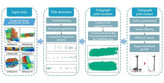
2.2.1. Pole Detection

In order to improve the efficiency of point cloud management and remove interference point clouds, including too high and too low non-pole-like point clouds, the filtered point cloud is segmented on a plane grid before the pole detection.

Plane grid segmentation refers to dividing a specific grid size, and each point is classified into the corresponding plane grid according to its $\left(x,y\right)$ coordinates. The z coordinate difference between the highest and the lowest points in each plane grid are employed to calculate the grid height difference, while point clouds with too large and too small height differences are removed based on the height threshold.

Since the poles are usually perpendicular to the ground, are isolated, and their vertical connectivity is good, the pole-shaped point cloud should be connected columnar in the vertical space after being divided by the plane grid. Therefore, all points in a single plane grid can be grown vertically upward, and the height of the point cloud growth can be utilized to detect the existence of a pole-shaped point cloud in the plane grid.

The point cloud in each two-dimensional grid is divided into a three-dimensional grid. Accordingly, the boundary value of the spatial grid where the point cloud in the area is located can be determined based on the maximum and minimum values of x, y, and z of the point cloud in the grid, and the division interval is then adjusted to divide all two-dimensional grids into three-dimensional ones. Then, the region downward growth algorithm aims to extract the pole-shaped point cloud based on region growth. The algorithm flow is as follows:

1.

Determining the seed grid: select the highest grid as the seed grid, and employ its number in the x, y, and z-axis directions as the grid coordinates $\left(r_0,c_0,l_0\right)$;

2.

Take the seed grid $\left(r_0,c_0,l_0\right)$ as the center. If the five-neighbor (front, back, left, right, and bottom) grid $\left(r,c,l\right)$ contains the point cloud data, continue to compare the number of points in the grid with the threshold. If it is greater than the threshold, merge the points in the $\left(r,c,l\right)$ and $\left(r_0,c_0,l_0\right)$ grids, and push the grid coordinates $\left(r,c,l\right)$. into the stack;

3.

Select a grid from the stack and take it as the seed grid in the first step, and repeat the second step;

4.

Repeat steps ②~③ until the stack becomes empty, and then complete the extraction of the point cloud-connected grid in a single plane grid.

As presented in the black box in Figure 3, the pole-shaped point cloud has good vertical connectivity, while the point cloud has poor connectivity, and its vertical spacing is relatively large, as the vegetation canopy. The above method can remove most of the point clouds with poor connectivity in the vertical direction.

2.2.2. Candidate Telegraph Pole Locating Based on Suspension Point in the Buffer Area

In addition to the telegraph poles extracted in the steps of Section 2.2.1, there are streetlights, vertical surfaces of buildings, tree trunks, and traffic signs. For a candidate telegraph pole, a location algorithm is proposed to extract its point cloud based on the suspension point in the buffer and the topological relationship between it and the pole, considering that the power suspension line is usually at a certain distance from the ground. The specific steps are:

• The pole’s central point is taken as the center of the circle and the point cloud between a certain distance as the point cloud of the buffer.
• The buffer point cloud is divided into n layers at a specific interval Δz along the z-axis, while the number of points in each layer is counted.
• Scan the points of each level from the top layer down. If the number of point clouds in the continuous local layer satisfies the rule of “greater than threshold-empty-greater than threshold-empty-greater than threshold”, the pole corresponding to the buffer zone is regarded as a candidate telegraph pole.

Figure 4a shows a point cloud diagram of a telegraph pole and a buffer area. The red, black, and green points indicate the telegraph pole point cloud, the telegraph pole center point, and the telegraph pole buffer point cloud obtained by segmentation, respectively. Figure 4b shows a statistical histogram of the number of points per layer, in which the abscissa of the histogram indicates the number of points per layer, while the ordinate is the layer number.

2.2.3. Telegraph Pole Locating Based on the Horizontal Projection of the Backbone Area

Generally, there is much vegetation around the poles in the distribution network. Since the buffer area at the top of the trunk is mainly the canopy, there is also an interval between the canopy leaves similar to the power suspension. If the pole is located based on the floating-point of the buffer area, the trunk can be easily misclassified into the pole. Therefore, accurate removal of the trunk points from the candidate telegraph pole point cloud is the main challenge of the telegraph pole locating. A telegraph pole locating algorithm based on the horizontal projection of the backbone area is adopted to solve the misclassification of telegraph poles and vegetation. The candidate telegraph pole point cloud is divided into independent clusters using European clustering. Consider that the upper part of the pole is usually connected to the power line, while the lower part is mainly connected to the surface objects like vegetation. Only the point cloud of the backbone of each type of cluster is projected to the horizontal plane to avoid interference between power lines and surface objects. Assuming that the length of the circumscribed rectangle of the vegetation trunk projection is much longer than that of the telegraph pole, the threshold of the circumscribed rectangle length is set to eliminate the vegetation point and complete the telegraph pole locating.

In Figure 5a,b, the red dots indicate the backbone area parts of vegetation and telegraph poles, respectively. In Figure 5b, the yellow and blue boxes indicate the parts where the pole is connected to the power line, and vegetation, respectively. Figure 5c,d describe the projections of the backbone area of vegetation and telegraph poles, respectively.

In Figure 6a, the black dots are the horizontal projection points of the backbone of a specific candidate telegraph pole, the blue dashed box indicates the maximum and minimum values of the point cloud data on the x and y axes, and the red dashed box is the actual circumscribed rectangle of the point cloud data. A significant error will occur while calculating the side length by determining the four corners of the circumscribed rectangle of the horizontal projection of the backbone if the corners of the point cloud data are determined according to their maximum and minimum values in the x and y-axis directions. Therefore, the coordinate system rotation method is employed to extract the corner coordinates of the point cloud data, and the side lengths of the circumscribed rectangle are then calculated as follows. Since the rectangle is a centrally symmetrical figure, the red dotted rectangle with the smallest area can be found within 90° of its coordinate origin, which is the actual circumscribed rectangle of the point cloud data, as shown in Formula (1), where $\left(x_0,y_0\right)$ and $\left(x,y\right)$ are the coordinates before and after the rotation and $\alpha$ is the angle of counterclockwise rotation. The four green points in Figure 6b are the corner points of the circumscribed rectangle of the black point cloud. By calculating the distance between adjacent corner points, the maximum distance is taken as the length of the circumscribed rectangle. If this length is less than the threshold, the cluster is judged as a pole point, and its center point coordinates are calculated.

$$\{\begin{array}{l}x=x_0\cos \alpha -y_0\sin \alpha \\ y=x_0\sin \alpha +y_0\cos \alpha \end{array}$$

(1)

2.2.4. Telegraph Pole Extraction Based on DBSCAN Algorithm

According to the spatial geometric characteristics and point cloud distribution characteristics of the telegraph poles and surrounding terrain features, the accurate extraction of the pole point cloud is realized through the following stages.

(1)

The buffer segmentation:

The points in the buffer zone of each pole are processed considering different environmental conditions around each telegraph pole. The buffer segmentation aims to establish a buffer zone in the non-ground point cloud after ground filtering, considering the center of the telephone pole and a certain distance as the center and the radius of the circle, respectively. The buffer segmentation result is shown in Figure 7.

(2)

Radius filtering:

Radius filtering is utilized to remove the noise points around the telegraph poles, considering the complexity of various spatial data structures and the efficiency of various indexing algorithms. Radius filtering refers to traversing every point in the buffer. If each point has at least N neighboring points within a specific search radius R, the point will be retained; otherwise, it will be removed. The noise points in the red dashed box in Figure 7a are removed and shown in Figure 7b. This method can effectively remove many discrete noise points around the telegraph poles and avoid interference in subsequent operations.

(3)

DBSCAN clustering:

The telegraph pole point cloud in the buffer zone is dense and uniform, and its shape is regular. The DBSCAN algorithm [27], which can detect clusters with arbitrary shapes and densities, is suitable for segmentation of the telegraph pole point cloud in the buffer. The key idea of the DBSCAN algorithm is: for each cluster point, the neighborhood of a given search radius ε must contain at least the minimum number of minPts points; that is, the density in the neighborhood must exceed a certain threshold. The distance function between two points p and q, denoted by dist(p, q), determines the shape of the neighborhood. This article employs the Euclidean distance in three-dimensional space. Since the total number of telegraph pole point clouds is greater than the number of various points, the clusters with the most points are retained. Figure 8 shows the DBSCAN clustering effect, where different clusters are indicated with different colors.

(4)

Region downward growth:

The region downward growth algorithm described in Section 2.2.1 can extract the telegraph pole point cloud. Formula (2) calculates the seed points of the algorithm. The point cloud in the connected grid can be extracted through the spatial grid growing to the left, right, forward, backward, and downward.

$$\{\begin{array}{l}see{d}_{down}.x=center.x\\ see{d}_{down}.y=center.y\\ see{d}_{down}.z=max.z\end{array}$$

(2)

where $see{d}_{down}$ is the seed point; $center$ is the center point of a telegraph pole; $max$ is the highest point in the buffer area; x, y and z are the x, y and z coordinates of the point, respectively.

2.2.5. Accuracy Evaluation

(1)

Telegraph pole locating

The evaluation content of the locating result includes two parts. One is the detection accuracy, which means the difference between the number of telegraph poles extracted by the algorithm and the number of true ones. The second is the locating deviation, which means the deviation between the plane position of the telegraph poles extracted by the algorithm and the true one.

In order to quantitatively evaluate the detection accuracy of utility poles, several indicators, including Recall, Precision, and F1-score [28] are employed to evaluate the algorithm’s performance. Recall represents the percentage of telegraph pole objects correctly detected from the telegraph poles on the ground. The percentage of telegraph pole objects that are correctly detected in all test results is described with Precision. F1-score is the harmonic average of Precision and Recall. These indices can be obtained through relations (3)–(5).

$$Recall=\frac{TP}{TP+FN}$$

(3)

$$Precision=\frac{TP}{TP+FP}$$

(4)

$$F1=2\times \frac{Recall\times Precision}{Recall+Precision}$$

(5)

where TP, FN, and FP represent the number of correctly detected, undetected, and incorrectly detected telegraph poles in the results, respectively.

The Root Mean Square Error (RMSE) [29] index is utilized to calculate the plane positioning error of the telegraph pole that the algorithm can correctly detect while quantitatively assessing the telegraph pole positioning deviation. The calculation formula is shown in Equation (6).

$$RMSE=\sqrt{\frac{{\displaystyle \sum _{i=1}^n{\left(d_i-d_{ir}\right)}^2}}{n}}$$

(6)

where $d_i=\sqrt{{\left(x_{ci}-x_{ri}\right)}^2+{\left(y_{ci}-y_{ri}\right)}^2}$, $i=1,2,\cdots ,n$ is the difference between the position of the i-th telegraph pole calculated by the algorithm and the true one, and n is the total number of telegraph poles that the algorithm can correctly detect.

(x_ci, y_ci) is the position of the i-th telephone pole calculated by the algorithm.$\left(x_{ri},y_{ri}\right)$ is the true position of the i-th telephone pole, calculated by the Formula (7).

$$\{\begin{array}{l}{x}_{ri}=\frac{{\displaystyle \sum _{j=1}^k{x}_j}}{k}\\ y_{ri}=\frac{{\displaystyle \sum _{j=1}^k{y}_j}}{k}\end{array}$$

(7)

where (x_j, y_j), j = 1, 2, ..., k are the point coordinates of the i-th telegraph pole, and k is the total number of points of the i-th telegraph pole.

(2)

Telegraph pole extraction

Although Recall, Precision, and F1-score are also employed as the evaluation indicators of the extraction results, they have different meanings from the parameters in the telegraph pole locating evaluation formula. In the calculation formula of the evaluation indices for the extraction result of the telephone poles, Recall represents the percentage of the correctly detected telegraph pole points in the true points of the pole, and Precision represents the percentage of correctly detected pole points in all the detected points. TP, FN, and FP represent the number of correctly detected, undetected, and incorrectly detected telegraph pole points in the results, respectively.

3. Results

The data of six experimental areas presented in Section 2.1 are utilized for qualitative and quantitative analysis to evaluate the effectiveness and robustness of the proposed method in locating and extracting telegraph poles. The telegraph pole location and extraction software was written in C++ and was run on a DELL desktop computer with Intel(R) Core(TM) i7-10700 CPU @2.90GHz, and 24.0 GB RAM.

The filtering algorithm divides the original point cloud into the ground and non-ground points. The results are shown in Figure 9a,b. The results of telegraph pole detection, pole location, and pole extraction of non-ground points are then displayed, and their accuracy is evaluated.

3.1. Telegraph Pole Location Result

(1)

Pole detection result

Plane grid segmentation is performed for non-ground points. In order to increase the running speed to ensure the segmentation effect, the grid length and width are both set to 1.5 m after repeated experiments. The height difference between the highest and lowest points in the vertical space is calculated in a single plane grid. The plane grids that are too high (above 25 m) and too low (below 4 m) are removed, considering that the height of the distribution network cement poles is between 6–20 m. The connected components of a single plane grid are analyzed after segmentation. According to the point cloud density, the grid’s length, width, and height in the region downward growth algorithm are all set to 0.3 m, while the vertical height threshold of the connected points obtained from the regional growth is 4 m. The pole detection result is shown in Figure 10, where the blue and red points represent the pole point cloud and the center point of the pole plane projection, respectively. Since the vegetation leaves are not continuous in the vertical structure, the grid containing vegetation leaves can be eliminated. Finally, a point cloud of poles, including telegraph poles, tree trunks, and street lights, is obtained.

(2)

Result of candidate telegraph pole location

In this experiment, the center of a single pole is taken as the center, while the area between 2.5–4 m from the circle’s center is taken as the buffer area. The buffer point cloud is shown as the green points in Figure 10. The green points in Figure 11 indicate the proposed method’s candidate telegraph pole point cloud.

(3)

Telegraph pole location result

The telegraph pole location algorithm based on the horizontal projection of the backbone area proposed in Section 2.2.3 eliminates the trunk points. In selecting the backbone, one-third to one-half of each cluster is taken as the backbone (indicated by the blue dots in Figure 11) to avoid the interference of power lines and surface objects on the extraction of telegraph poles and consider the spatial structure of vegetation. After denoising the main part, it is projected to the horizontal plane. The coordinate system rotation method is employed to calculate the length of the circumscribed rectangle of the main part of the point cloud after projection, and the length threshold is set to 1.5 m according to the design code for the diameter of the pole-shaped pole. If the calculated length of the circumscribed rectangle is less than the threshold, the cluster will be judged as a telegraph pole point cloud, and its center point coordinates will be calculated. Figure 12 shows the location results of the pole, where the green and red points indicate the pole point cloud, and the pole’s center point, respectively.

(4)

Quantitative evaluation

Table 2. Detection accuracy of telegraph poles.

Dataset Number	TP	FP	FN	Recall (%)	Precision (%)	F1-Score (%)
Dataset-I	10	1	1	90.91	90.91	90.91
Dataset-II	33	3	2	94.29	91.67	92.96
Dataset-III	6	1	1	85.71	85.71	85.71
Dataset-IV	10	1	2	83.33	90.91	86.96
Dataset-V	5	0	0	100.00	100.00	100.00
Dataset-VI	12	2	1	92.31	85.71	88.89

shows the detection accuracy of utility telegraph poles. The Recall values of Dataset-I to Dataset-VI are 90.91%, 94.29%, 85.71%, 83.33%, 100.00%, and 92.31%, while the Precision values are 90.91%, 91.67%, 85.71%, 90.91%, 100.00%, and 85.71%, respectively. F1-score values are 90.91%, 92.96%, 85.71%, 86.96%, 100.00%, and 88.89%, respectively. Since the image matching point cloud will have missing power lines at the edge, there is a significant difference between Recall, Precision, and F1-score in each dataset. It is challenging for the algorithm to locate the telegraph poles when they are not connected to the suspension wires. However, the average values of Recall, Precision, and F1-score can still reach 91.09%, 90.82%, and 90.90%, respectively, indicating the effectiveness of the proposed method for the detection of telegraph poles.

Table 3. Location deviation of telegraph poles for the six datasets.

Dataset Number	Minimum (m)	Maximum (m)	Average (m)	RMSE (m)
Dataset-I	0.078782	1.02	0.50	0.59
Dataset-II	0.038589	1.34	0.32	0.43
Dataset-III	0.225596	1.05	0.53	0.63
Dataset-IV	0.022969	0.50	0.20	0.23
Dataset-V	0.096417	0.41	0.25	0.50
Dataset-VI	0.066732	1.10	0.43	0.66

shows the minimum, maximum, average, and RMSE of the location deviation of the six datasets. The RMSE values are 0.59 m, 0.43 m, 0.63 m, 0.23 m, 0.50 m, and 0.66 m, respectively. It is necessary to divide the radius with the telegraph pole’s plane coordinates as the center while extracting telegraph poles. However, since the radius during the radius division is set to 5m in subsequent experiments, the radius division can still cover all the true telegraph pole points even if the maximum positioning error occurs.

3.2. Telegraph Pole Extraction Results

Four telegraph pole point cloud data are selected from the experimental data, and the method described in Section 2.2.4 is employed for experimental analysis. The main parameter settings are shown in

Table 4. Pole extracting parameters.

Step	Parameters
	Name	Value
Buffer segmentation	Radius(m)	5
Remove filtering	Radius (m)	0.04
	Minimum points	5
DBSCAN cluster	Radius(m)	0.4
	Minimum points	5
Region growing	Grid length(m)	0.1
	Grid width(m)	0.1
	Grid height(m)	0.1

.

Figure 13a–d describes the extraction process of four poles. The ① and ② images are the projection images of the point cloud in the buffer zone of the telephone pole on the XZ and YZ planes, respectively. The ③ and ④ images are the projection images of the point cloud data after the radius denoising on the XZ and YZ planes. The ⑤ and ⑥ show the projection images of the clusters with the largest number of points in the DBSCAN clustering results on the XZ and YZ planes, respectively. The algorithm can effectively remove the suspension lines and vegetation around the poles. The ⑦ and ⑧ images are the projection images of the point cloud obtained through the region downward growth algorithm on the XZ and YZ planes. This method can obtain a smoother pole-shaped structure. Comparing the ⑦ and ⑧ images with the ① and ② images indicates that the algorithm can eliminate the noise around the pole and precisely extract its point cloud data.

Table 5. The telegraph pole extraction results.

Dataset Number	TP	FP	FN	Recall (%)	Precision (%)	F1-Score (%)	Total Times
Dataset-I	23,603	1951	2767	89.51	92.37	90.91	0.90
Dataset-II	215,796	21,484	19,840	91.58	90.95	91.26	29.64
Dataset-III	18,417	1935	1371	93.07	90.49	91.76	0.53
Dataset-IV	9378	1016	1069	89.77	90.23	90.00	0.39
Dataset-V	16,194	427	1241	92.88	97.43	95.10	1.10
Dataset-VI	39,436	2950	3950	90.90	93.04	91.96	3.73

shows the telegraph pole extraction results in six datasets. The F1-score values of telegraph poles I-VI after point cloud extraction are 90.91%, 91.26%, 91.76%, 90.00%, 95.10%, and 91.96%, respectively, while the extraction times are 0.90 s, 29.64 s, 0.53 s, 0.39 s, 1.10 s, and 3.73 s. The DBSCAN algorithm provides a higher extraction accuracy and efficiency in the extraction process. This is because the extraction algorithm extracts the telegraph poles and their surrounding points without employing the DBSCAN algorithm for the entire large scene.

4. Discussion

In order to evaluate the impact of critical parameters on the algorithm and verify its robustness, different parameter settings are chosen for sensitivity analysis during the region downward growth while locating the candidate telegraph poles based on the buffer floating-point and DBSCAN clustering. The telegraph pole locating and extracting algorithms are evaluated through Dataset-I and pole I, respectively. Each experiment only changes the test parameter values and sets the other parameters as default values.

4.1. The Influence of the Length, Width, and Height of the Spatial Grid on Pole Detection

The spatial grid’s length, width, and height directly affect the height of the point cloud that can be connected in the vertical space. The spatial grid is designed as a square with side lengths of 0.1 m, 0.2 m, 0.3 m, 0.4 m, and 0.5 m. Figure 14 indicates the effect of the algorithm on the extraction of telegraph poles under different grid sizes. On the one hand, if the grid is small and the point cloud density is low, it is easy to make the side length of the grid smaller than the point spacing, and it is challenging to include the pole-shaped points that are far apart into the stack when the grid grows. Accordingly, the height of the connected point cloud is much smaller than the actual height of the pole, resulting in missing points. On the other hand, if the grid is too large and the area grows downwards, it is easy to grow the branches and leaves with a large vertical interval of vegetation to the same stack, resulting in misclassification. Therefore, the spatial grid’s length, width, and height are chosen as 0.3 m.

4.2. The Influence of Buffer Distance Threshold on the Telegraph Pole Locating

The correct judgment of the buffer’s power suspension is the key to extracting the candidate telegraph poles. The minimum distance threshold is adjusted to 2.5 m, 2 m, 2.5 m, 3 m, and 3.5 m. As shown in Figure 15, both too large and too small thresholds will decrease the F1-score. The reason is that when the minimum distance is set too small, it is easy to incorporate the pole attachment parts into the buffer area. In contrast, when the minimum distance is set too large, it is easy to draw the vegetation around the pole into the buffer area. It is challenging to identify the power suspension line correctly in both cases, leading to leakage. The maximum distance threshold is 3 m, 3.5 m, 4 m, 4.5 m, and 5 m. The smaller the maximum distance setting, the lower the F1-score. This is because the employed data is the point cloud obtained by dense image matching, and there is a partial lack of the power suspension line point cloud directly connected to the pole. The smaller the maximum distance threshold, the smaller the buffer area, while there will be fewer power suspension line points in the buffer, quickly leading to leakage. Therefore, this paper employs the experimental results to set the minimum and maximum distance thresholds to 2.5 m and 4 m, respectively.

The average F1-score value in the test results of different parameters is 92%, demonstrating the proposed algorithm’s strong applicability and high robustness.

4.3. The Influence of Radius on the Telegraph Pole Extraction

The search radius in the DBSCAN algorithm determines the neighborhood range of a point. The search radius is set to 0.1 m, 0.2 m, 0.3 m, 0.4 m, 0.5 m, 0.6 m, 0.7 m, and 0.8 m. As shown in Figure 16, the F1-score values are greater than 91% for the search radius in the range 0.1–0.5 m. When the search radius is greater than 0.5 m, the noise points around the telegraph poles are misclassified as pole points, which increases the number of detected error points, and rapidly reduces the F1-score value to 55.9%. Therefore, the search radius is taken as 0.4 m in this paper.

5. Conclusions

The telegraph pole point cloud has information like location and geometric shape, providing primary data for the intelligent management and maintenance of the distribution network and construction planning. There are often interfering features like trees and light poles on the distribution network lines, resulting in misclassification of the point cloud extraction results of the telegraph poles. Besides, although LiDAR can obtain accurate point cloud data, it cannot acquire a telegraph pole point cloud due to its high price. This paper proposes a pole location and extraction method based on point cloud generated through dense image matching, including pole detection, candidate telegraph pole location, and precise locating and extracting of telegraph poles, to overcome the above problems. First, the grid segmentation and connected component analysis are performed on the non-ground points generated after filtering to achieve pole detection. The point cloud in the pole buffer is then vertically layered. If there is a layer with empty points, the center of the current pole is utilized as the location of the candidate telegraph pole. Finally, the candidate telegraph pole backbone point cloud is projected to the horizontal plane, and the circumscribed rectangle is calculated. The point cloud whose rectangle length is less than the threshold is regarded as a telegraph pole point cloud. Moreover, to extract the telegraph pole, buffer segmentation, radius filtering, DBSCAN clustering, and region downward growth algorithms are adopted. The precise locating and extraction of the telegraph pole can be evaluated using the above methods. Various experiments were performed on Dataset-I to Dataset-VI to evaluate the performance of the proposed method. The experimental results demonstrate that the average values of Recall, Precision, and F1-score in telegraph pole detection can still reach 91.09%, 90.82%, and 90.90%, respectively. The average RMSE value of location deviation is 0.51m. The average value of the F1-score in the telegraph pole extraction result is 91.83%, and the average extraction time of a single pole is 0.27s. It indicates that the method can accurately extract most of the telegraph pole point clouds faster.

The main advantages of the proposed method are:

(1)

Assuming that the top of the pole is connected to the power suspension line, the telegraph pole point cloud is clearly distinguished from that of other poles, which effectively removes interfering ground objects and guarantees the recall rate of the telegraph pole detection effectively.

(2)

Assuming that the horizontal projection area of the tree canopy is larger than the telegraph pole, the tree point cloud is further filtered out to improve the extraction accuracy.

(3)

Compared with the point cloud collected by LiDAR, point cloud generation based on dense image matching reduces the cost, and it is suitable for popularization and application in distribution network inspection.

Although the proposed method achieves a high accuracy and recall rate for locating and extracting telegraph poles, it is necessary to collect point cloud data of distribution network lines with larger data scales and more complex environments in subsequent research to perform a more comprehensive evaluation of the proposed method.

References

1. Guo, B.; Huang, X.; Li, Q.; Zhang, F.; Zhu, J.; Wang, C. A stochastic geometry method for pylon reconstruction from airborne lidar data. Remote Sens. 2016, 8, 243. [Google Scholar] [CrossRef] [Green Version]
2. Conde, B.; Villarino, A.; Cabaleiro, M.; Gonzalez-Aguilera, D. Geometrical issues on the structural analysis of transmission electricity towers thanks to laser scanning technology and finite element method. Remote Sens. 2015, 7, 11551–11569. [Google Scholar] [CrossRef] [Green Version]
3. You, A.; Wang, X.; Han, X.; Tang, D. Applications of LiDAR in patrolling electric-power lines. In Proceedings of the 2013 The International Conference on Technological Advances in Electrical, Electronics and Computer Engineering (TAEECE), Konya, Turkey, 9–11 May 2013; pp. 110–114. [Google Scholar]
4. Qin, X.; Wu, G.; Lei, J.; Fan, F.; Ye, X. Detecting inspection objects of power line from cable inspection robot LiDAR data. Sensors 2018, 18, 1284. [Google Scholar] [CrossRef] [Green Version]
5. Rhee, S.; Kim, T. Dense 3D point cloud generation from UAV images from image matching and global optimazation. Int. Arch. Photogramm. Remote Sens. Spat. Inf. Sci. 2016, 41, 1005. [Google Scholar] [CrossRef] [Green Version]
6. Rosnell, T.; Honkavaara, E. Point cloud generation from aerial image data acquired by a quadrocopter type micro unmanned aerial vehicle and a digital still camera. Sensors 2012, 12, 453–480. [Google Scholar] [CrossRef] [Green Version]
7. Rothermel, M.; Haala, N. Potential of dense matching for the generation of high quality digital elevation models. In Proceedings of the ISPRS Workshop High-Resoultion Earth Imaging for Geospatial Information; ISPRS: Hannover, Germany, 2011. [Google Scholar]
8. Kang, Z.; Yang, J.; Zhong, R.; Wu, Y.; Shi, Z.; Lindenbergh, R. Voxel-based extraction and classification of 3-D pole-like objects from mobile LiDAR point cloud data. IEEE J. Sel. Top. Appl. Earth Obs. Remote Sens. 2018, 11, 4287–4298. [Google Scholar] [CrossRef]
9. Teo, T.-A.; Chiu, C.-M. Pole-like road object detection from mobile lidar system using a coarse-to-fine approach. IEEE J. Sel. Top. Appl. Earth Obs. Remote Sens. 2015, 8, 4805–4818. [Google Scholar] [CrossRef]
10. Yadav, M.; Lohani, B.; Singh, A.K.; Husain, A. Identification of pole-like structures from mobile lidar data of complex road environment. Int. J. Remote Sens. 2016, 37, 4748–4777. [Google Scholar] [CrossRef]
11. Yan, W.Y.; Morsy, S.; Shaker, A.; Tulloch, M. Automatic extraction of highway light poles and towers from mobile LiDAR data. Opt. Laser Technol. 2016, 77, 162–168. [Google Scholar] [CrossRef]
12. Yan, L.; Li, Z.; Liu, H.; Tan, J.; Zhao, S.; Chen, C. Detection and classification of pole-like road objects from mobile LiDAR data in motorway environment. Opt. Laser Technol. 2017, 97, 272–283. [Google Scholar] [CrossRef]
13. McCulloch, J.; Green, R. Extraction of utility poles in LIDAR scans using cross-sectional slices. In Proceedings of the 2016 International Conference on Image and Vision Computing New Zealand (IVCNZ), Palmerston North, New Zealand, 21–22 November 2016; pp. 1–4. [Google Scholar]
14. Yang, J.; Kang, Z.; Akwensi, P.H. A skeleton-based hierarchical method for detecting 3-D pole-like objects from mobile LiDAR point clouds. IEEE Geosci. Remote Sens. Lett. 2018, 16, 801–805. [Google Scholar] [CrossRef]
15. Li, Y.; Wang, W.; Li, X.; Xie, L.; Wang, Y.; Guo, R.; Xiu, W.; Tang, S. Pole-like street furniture segmentation and classification in mobile LiDAR data by integrating multiple shape-descriptor constraints. Remote Sens. 2019, 11, 2920. [Google Scholar] [CrossRef] [Green Version]
16. Yu, Y.; Guan, H.; Li, D.; Jin, S.; Chen, T.; Wang, C.; Li, J. 3-D feature matching for point cloud object extraction. IEEE Geosci. Remote Sens. Lett. 2019, 17, 322–326. [Google Scholar] [CrossRef]
17. Zhang, X.; Liu, H.; Li, Y.; Wu, Z.; Mao, J.; Liu, Y. Streetlamp extraction and identification from mobile LiDAR point cloud scenes. In Proceedings of the 2016 IEEE International Geoscience and Remote Sensing Symposium (IGARSS), Beijing, China, 10–15 July 2016; pp. 1468–1471. [Google Scholar]
18. Shi, Z.; Kang, Z.; Lin, Y.; Liu, Y.; Chen, W. Automatic recognition of pole-like objects from mobile laser scanning point clouds. Remote Sens. 2018, 10, 1891. [Google Scholar] [CrossRef] [Green Version]
19. Zhang, R.; Yang, B.; Xiao, W.; Liang, F.; Liu, Y.; Wang, Z. Automatic extraction of high-voltage power transmission objects from UAV lidar point clouds. Remote Sens. 2019, 11, 2600. [Google Scholar] [CrossRef] [Green Version]
20. Li, Q.; Chen, Z.; Hu, Q. A model-driven approach for 3D modeling of pylon from airborne LiDAR data. Remote Sens. 2015, 7, 11501–11524. [Google Scholar] [CrossRef] [Green Version]
21. Guan, H.; Yu, Y.; Li, J.; Ji, Z.; Zhang, Q. Extraction of power-transmission lines from vehicle-borne lidar data. Int. J. Remote Sens. 2016, 37, 229–247. [Google Scholar] [CrossRef]
22. Shen, X.; Qian, C.; Du, Y.; Yu, X.; Zhang, R. An automatic extraction algorithm of high voltage transmission lines from airborne LIDAR point cloud data. Turk. J. Electr. Eng. Comput. Sci. 2018, 26, 2043–2055. [Google Scholar] [CrossRef]
23. Peng, X.; Song, S.; Qian, J.; Chen, C.; Wang, K.; Yang, Y.; Zheng, X. Research on Automatic Positioning Algorithm of Power Transmission Towers Based on UAV LiDAR. Power Syst. Technol. 2017, 41, 3670–3677. [Google Scholar]
24. Ye, L.; Liu, Q.; Hu, Q. Research of power line fitting and extraction techniques based on LiDAR point cloud data. Geomat. Spat. Inf. Technol. 2010, 5, 30–34. [Google Scholar]
25. Jwa, Y.; Sohn, G. A piecewise catenary curve model growing for 3D power line reconstruction. Photogramm. Eng. Remote Sens. 2012, 78, 1227–1240. [Google Scholar] [CrossRef]
26. Zhu, X.; Wang, C.; Xi, X.; Wang, P.; Tian, X.; Yang, X. Hierarchical threshold adaptive for point cloud filter algorithm of moving surface fitting. Acta Geod. Et Cartogr. Sin. 2018, 47, 153–160. [Google Scholar]
27. Ester, M.; Kriegel, H.; Sander, J.; Xu, X. A density-based algorithm for discovering clusters in large spatial databases with noise. In Proceedings of the Second International Conference on Knowledge Discovery and Data Mining (KDD’96), Portland, OR, USA, 2–4 August 1996. [Google Scholar]
28. Chen, M.; Wu, J.; Liu, L.; Zhao, W.; Tian, F.; Shen, Q.; Zhao, B.; Du, R. DR-Net: An improved network for building extraction from high resolution remote sensing image. Remote Sens. 2021, 13, 294. [Google Scholar] [CrossRef]
29. Zhu, L.; Zhang, Y.; Wang, J.; Tian, W.; Liu, Q.; Ma, G.; Kan, X.; Chu, Y. Downscaling Snow Depth Mapping by Fusion of Microwave and Optical Remote-Sensing Data Based on Deep Learning. Remote Sens. 2021, 13, 584. [Google Scholar] [CrossRef]
Figure 1. Overview of the research area. (a) Dataset-I. (b) Dataset-II. (c) Dataset-III. (d) Dataset-IV. (e) Dataset-V. (f) Dataset-VI.
Remotesensing 14 00433 g001
Figure 2. Flow chart of location and extraction of multi-level telegraph poles.
Remotesensing 14 00433 g002
Figure 3. Partial cross-section view of the point cloud grid.
Remotesensing 14 00433 g003
Figure 4. Buffer and layer-by-layer point statistics: (a) point cloud of telegraph poles and the buffer area; (b) the total number of points on each layer in the buffer area.
Remotesensing 14 00433 g004
Figure 5. The location of the backbone area and its projection: (a) main view of vegetation; (b) main view of line pole; (c) top view of vegetation; (d) top view of line pole.
Remotesensing 14 00433 g005
Figure 6. Calculation of circumscribed rectangle: (a) schematic diagram of the plane projection; (b) corners of the circumscribed rectangle.
Remotesensing 14 00433 g006
Figure 7. Buffer point cloud and point cloud denoising results: (a) Projection of buffer point cloud to XZ plane. (b) The projection of the point cloud to the XZ plane after denoising.
Remotesensing 14 00433 g007
Figure 8. Schematic diagram of DBSCAN clustering: (a) Projection to the XZ plane. (b) Projection to the YZ plane.
Remotesensing 14 00433 g008
Figure 9. Non-ground points (green point) and ground points (brown point). (a) Dataset-I. (b) Dataset-II. (c) Dataset-III. (d) Dataset-IV. (e) Dataset-V. (f) Dataset-VI.
Remotesensing 14 00433 g009
Figure 10. Buffer around the pole. (a) Dataset-I. (b) Dataset-II. (c) Dataset-III. (d) Dataset-IV. (e) Dataset-V. (f) Dataset-VI.
Remotesensing 14 00433 g010
Figure 11. Location results of candidate telegraph poles. (a) Dataset-I. (b) Dataset-II. (c) Dataset-III. (d) Dataset-IV. (e) Dataset-V. (f) Dataset-VI.
Remotesensing 14 00433 g011
Figure 12. Locating results of telegraph poles. (a) Dataset-I. (b) Dataset-II. (c) Dataset-III. (d) Dataset-IV. (e) Dataset-V. (f) Dataset-VI.
Remotesensing 14 00433 g012
Figure 13. Telegraph pole extraction process: (a) The extraction process for telegraph pole I. (b) The extraction process for telegraph pole II. (c) The extraction process for telegraph pole III. (d) The extraction process for telegraph pole IV.
Remotesensing 14 00433 g013
Figure 14. F1-score values for different spatial grid sizes.
Remotesensing 14 00433 g014
Figure 15. F1-score values corresponding to the minimum and maximum distances of different buffers: (a) Minimum distance; (b) Maximum distance.
Remotesensing 14 00433 g015
Figure 16. F1-score values for different radius values.
Remotesensing 14 00433 g016