
3MRS: An Effective Coarse-to-Fine Matching Method for Multimodal Remote Sensing Imagery

 ,
,  ,
, 
 ,
,
Abstract
:
1. Introduction
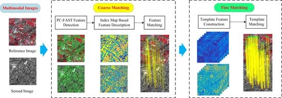
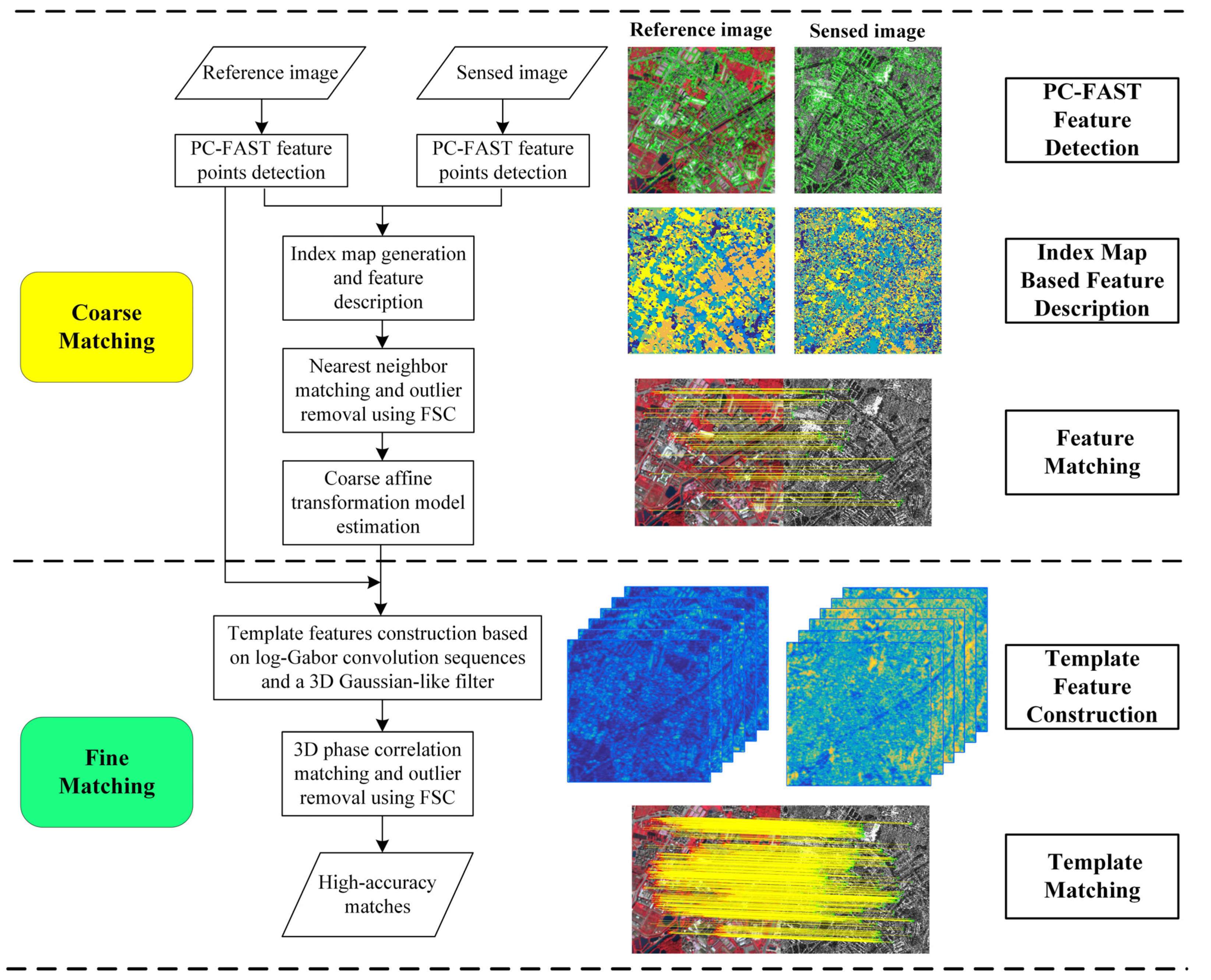
2. Methodology
2.1. Coarse Matching
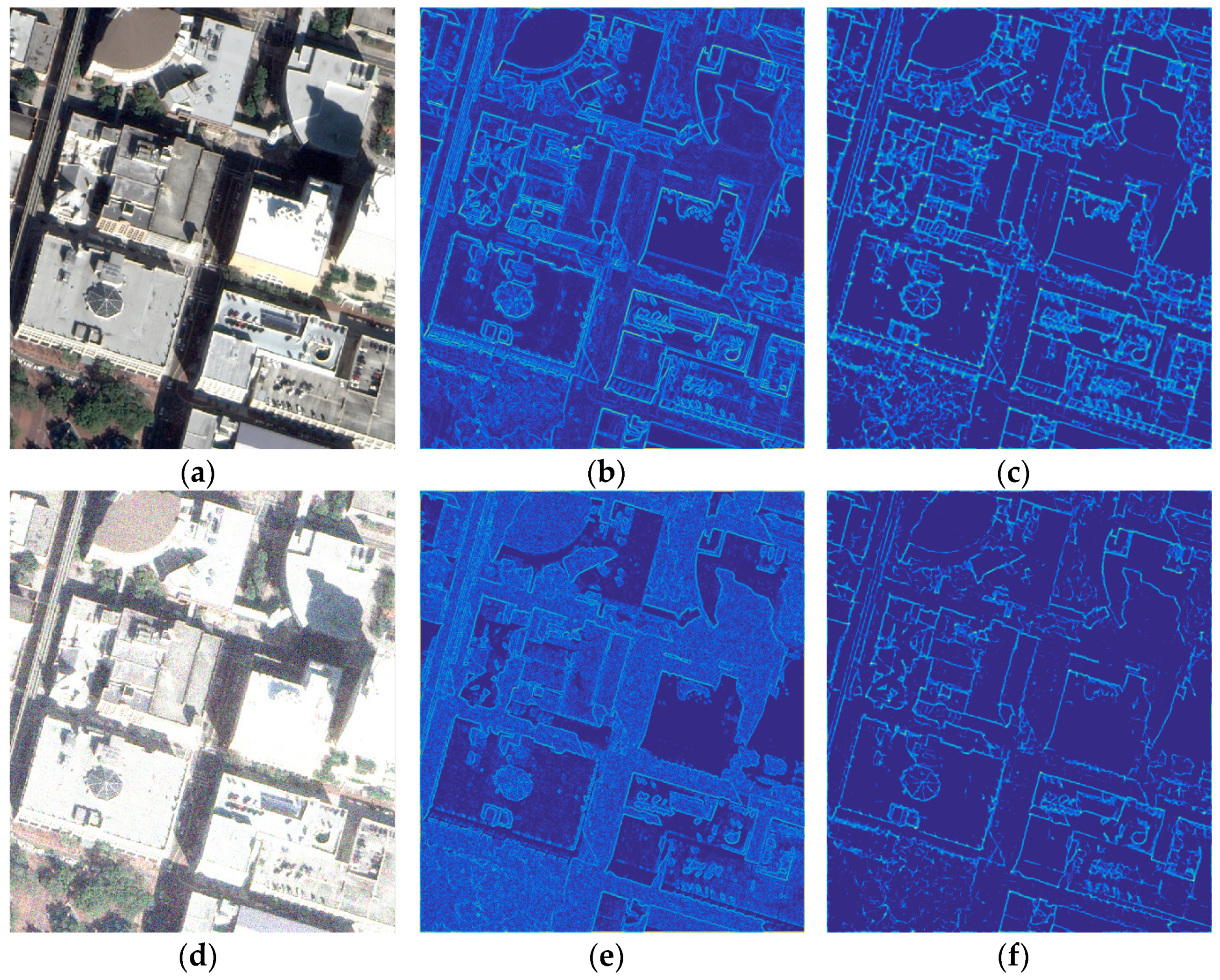
2.1.1. Point Feature Detection
2.1.2. Index-Map-Based Feature Description
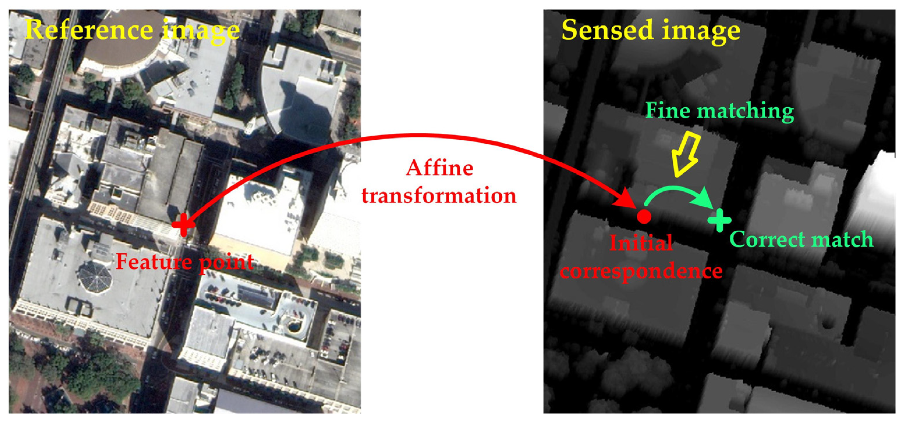
2.2. Fine Matching
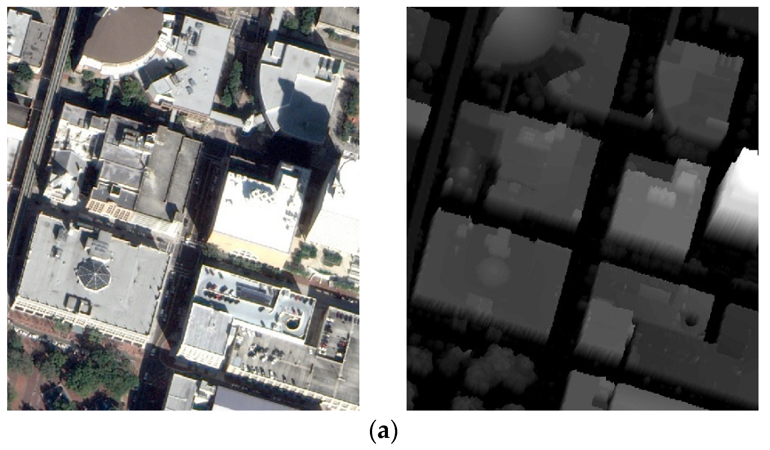
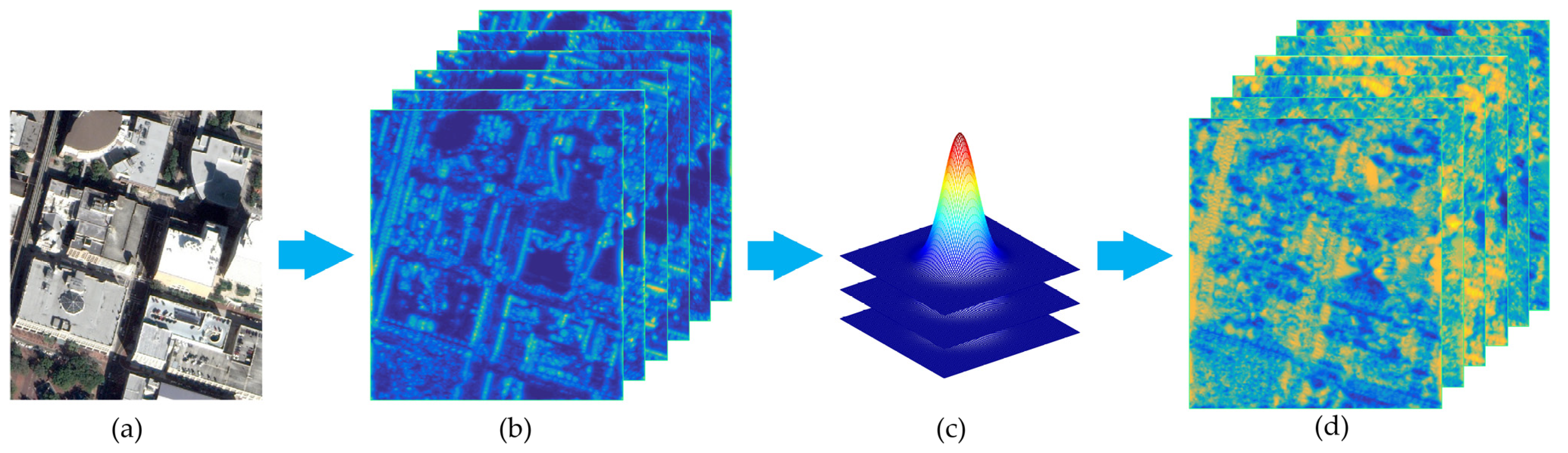
2.2.1. Template Feature Construction
2.2.2. 3D Phase Correlation Matching
3. Experiments and Results
3.1. Data Description
3.2. Evaluation Indices
- 1.
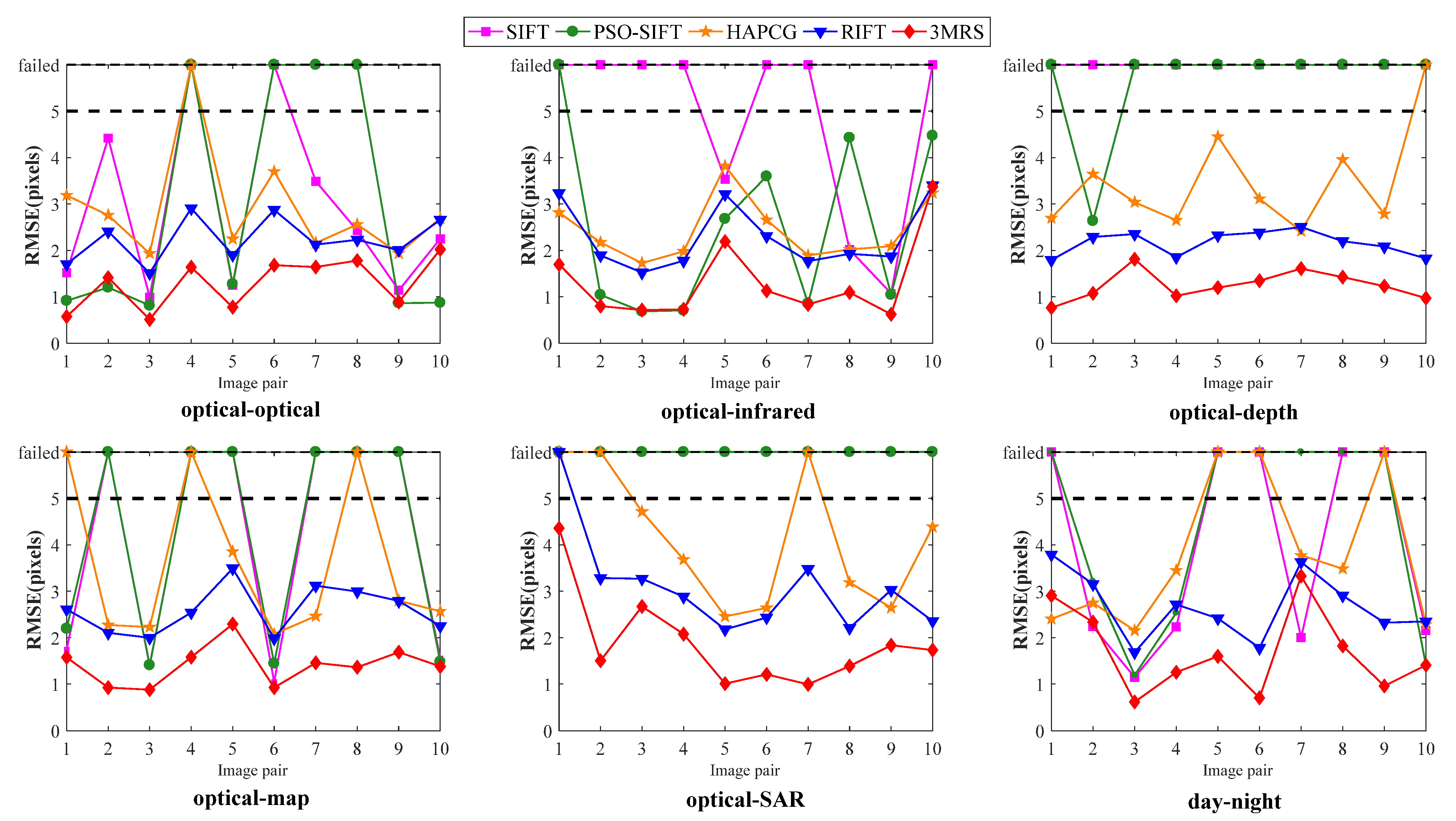
- SR refers to the ratio of the number of successfully matched image pairs to the total number of image pairs in a type of image pair. This index reflects the robustness of a matching method to a specific type of multimodal image pair.
- 2.
- To count the number of correct matches, we first use the obtained matches to estimate a transformation between an image pair. Then, the matches with residual errors of less than three pixels are taken as correct matches, and the number of correct matches is NCM. Additionally, the image pair with NCM smaller than three is deemed a matching failure. Considering the significant NID between multimodal remote sensing images, three pixels are a relatively strict threshold.
- 3.
- Taking the correct matches as input, the coordinates on one image can be converted to on the other image of the image pair using . If the coordinates of the corresponding matching point of are , RMSE can be calculated with (17). RMSE reflects the matching accuracy of the correct matches. The smaller the value of RMSE, the higher the accuracy. In addition, the image pairs with RMSE larger than five are deemed a matching failure.
- 4.
- With respect to efficiency, we not only count the total running time but also the time used for obtaining one correct match. Specifically, can be calculated as follows:
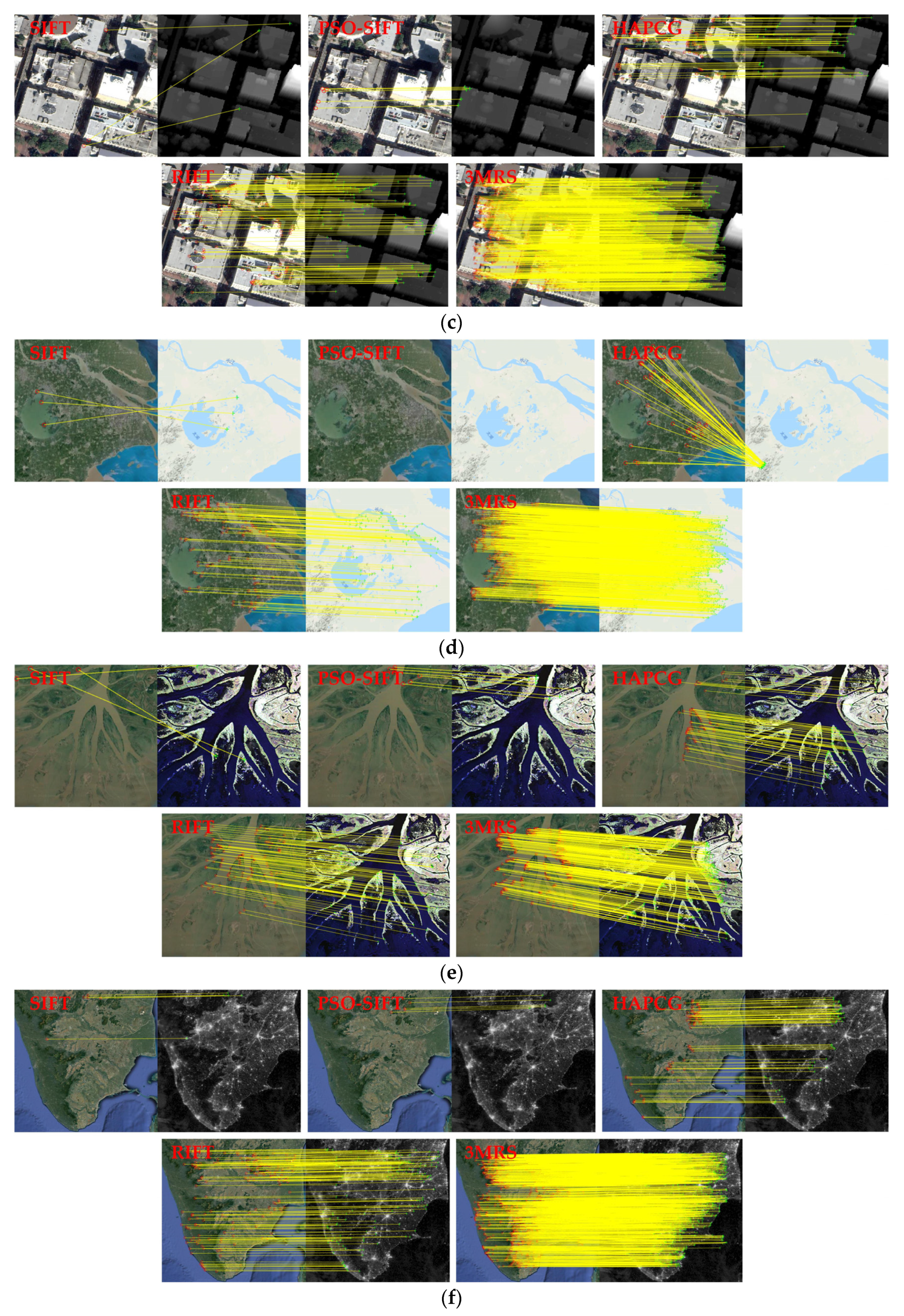
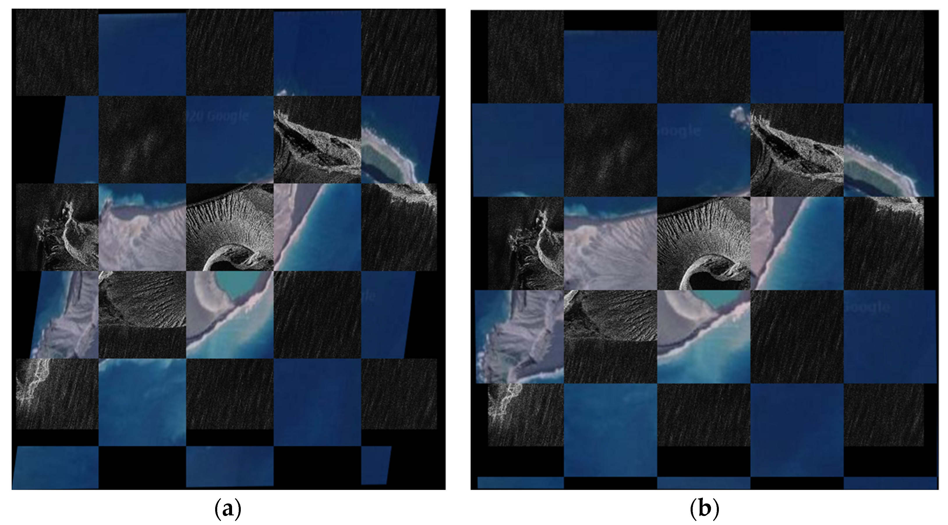
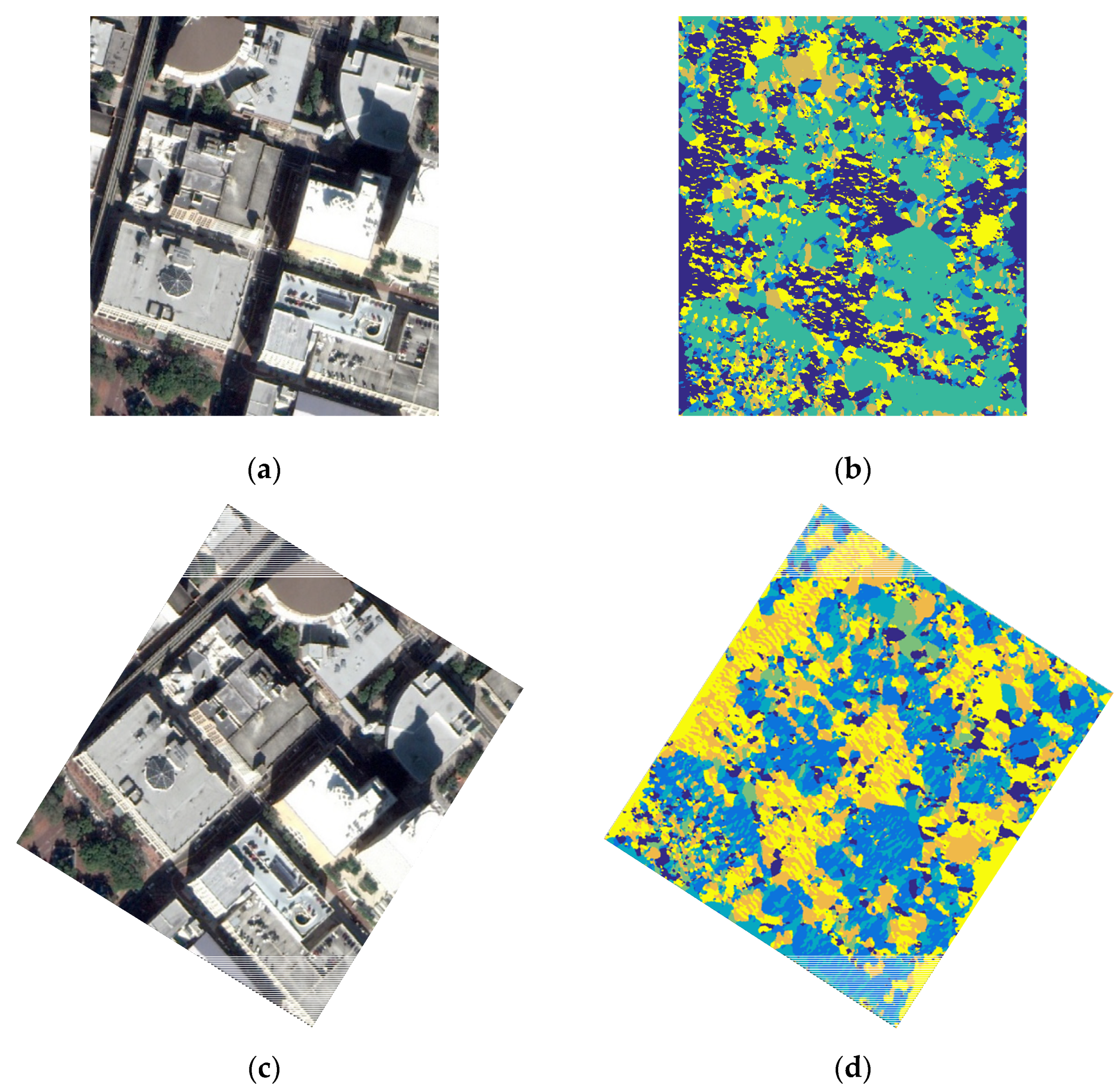
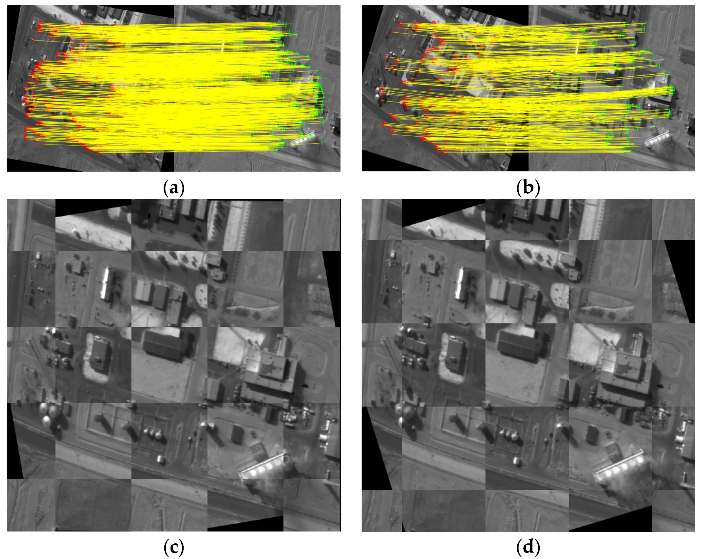
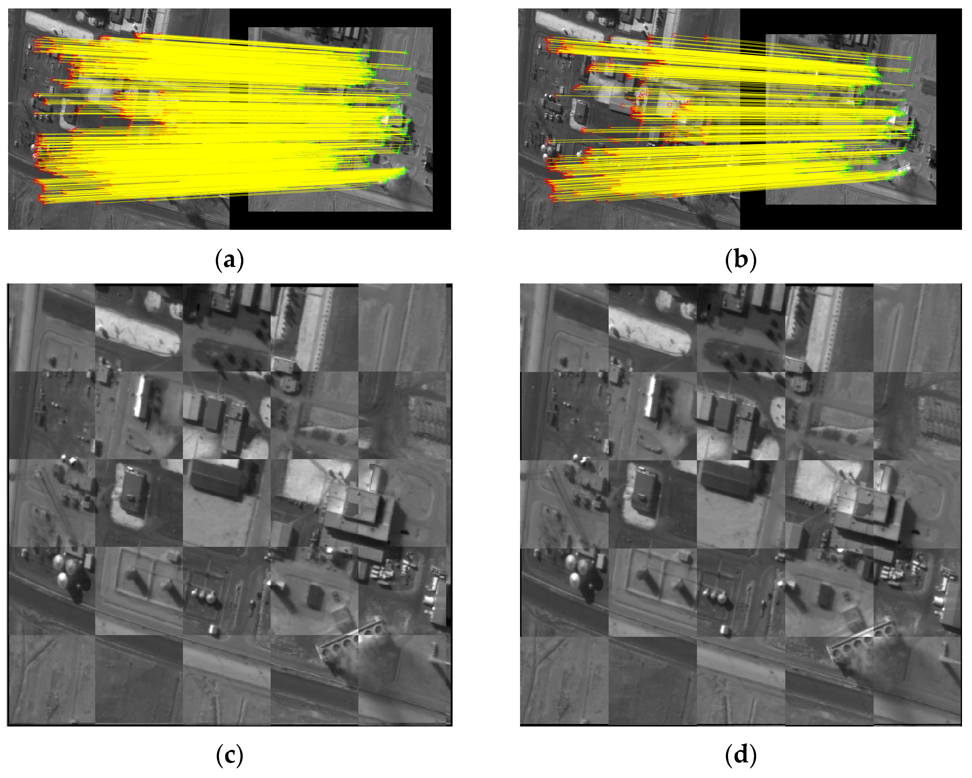
3.3. Qualitative Results
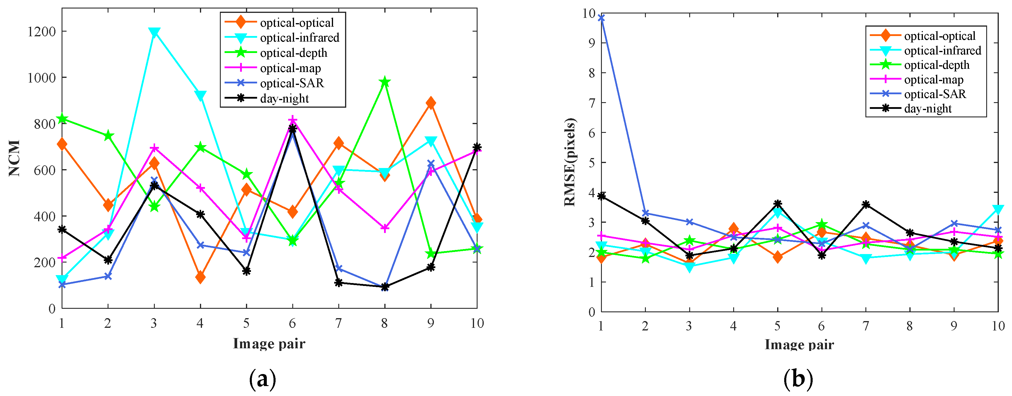
3.4. Quantitative Results
4. Discussion
4.1. Performance Analysis
4.2. The Influence of Coarse Matching on the Final Result
4.3. Performance of 3MRS with Respect to Rotation and Scale Change
5. Conclusions
Author Contributions
Funding
Institutional Review Board Statement
Informed Consent Statement
Data Availability Statement
Acknowledgments
Conflicts of Interest
References
- Zhou, K.; Lindenbergh, R.; Gorte, B.; Zlatanova, S. LiDAR-guided dense matching for detecting changes and updating of buildings in Airborne LiDAR data. ISPRS J. Photogramm. Remote Sens. 2020, 162, 200–213. [Google Scholar] [CrossRef]
- De Alban, J.D.T.; Connette, G.M.; Oswald, P.; Webb, E.L. Combined Landsat and L-band SAR data improves land cover classification and change detection in dynamic tropical landscapes. Remote Sens. 2018, 10, 306. [Google Scholar] [CrossRef] [Green Version]
- Niu, X.; Gong, M.; Zhan, T.; Yang, Y. A conditional adversarial network for change detection in heterogeneous images. IEEE Geosci. Remote Sens. 2018, 16, 45–49. [Google Scholar] [CrossRef]
- Touati, R.; Mignotte, M.; Dahmane, M. Multimodal change detection in remote sensing images using an unsupervised pixel pairwise-based Markov random field model. IEEE Trans. Image Process. 2019, 29, 757–767. [Google Scholar] [CrossRef] [PubMed]
- Chen, H.; Li, Y.; Su, D. Multimodal fusion network with multi-scale multi-path and cross-modal interactions for RGB-D salient object detection. Pattern Recognit. 2019, 86, 376–385. [Google Scholar] [CrossRef]
- Sharma, M.; Dhanaraj, M.; Karnam, S.; Chachlakis, D.G.; Ptucha, R.; Markopoulos, P.P.; Saber, E. YOLOrs: Object Detection in Multimodal Remote Sensing Imagery. IEEE J. Sel. Top. Appl. Earth Obs. Remote Sens. 2020, 14, 1497–1508. [Google Scholar] [CrossRef]
- Deng, Z.; Sun, H.; Zhou, S.; Zhao, J.; Lei, L.; Zou, H. Multi-scale object detection in remote sensing imagery with convolutional neural networks. ISPRS J. Photogramm. Remote Sens. 2018, 145, 3–22. [Google Scholar] [CrossRef]
- Liu, S.; Qi, Z.; Li, X.; Yeh, A.G.-O. Integration of convolutional neural networks and object-based post-classification refinement for land use and land cover mapping with optical and SAR data. Remote Sens. 2019, 11, 690. [Google Scholar] [CrossRef] [Green Version]
- Shao, Z.; Zhang, L.; Wang, L. Stacked sparse autoencoder modeling using the synergy of airborne LiDAR and satellite optical and SAR data to map forest above-ground biomass. IEEE J. Sel. Top. Appl. Earth Obs. Remote Sens. 2017, 10, 5569–5582. [Google Scholar] [CrossRef]
- Zhang, H.; Xu, R. Exploring the optimal integration levels between SAR and optical data for better urban land cover mapping in the Pearl River Delta. Int. J. Appl. Earth Obs. Geoinf. 2018, 64, 87–95. [Google Scholar] [CrossRef]
- Campos-Taberner, M.; García-Haro, F.J.; Camps-Valls, G.; Grau-Muedra, G.; Nutini, F.; Busetto, L.; Katsantonis, D.; Stavrakoudis, D.; Minakou, C.; Gatti, L. Exploitation of SAR and optical sentinel data to detect rice crop and estimate seasonal dynamics of leaf area index. Remote Sens. 2017, 9, 248. [Google Scholar] [CrossRef] [Green Version]
- Hong, D.; Hu, J.; Yao, J.; Chanussot, J.; Zhu, X.X. Multimodal remote sensing benchmark datasets for land cover classification with a shared and specific feature learning model. ISPRS J. Photogramm. Remote Sens. 2021, 178, 68–80. [Google Scholar] [CrossRef] [PubMed]
- Jiang, X.; Ma, J.; Xiao, G.; Shao, Z.; Guo, X. A review of multimodal image matching: Methods and applications. Inf. Fusion 2021, 73, 22–71. [Google Scholar] [CrossRef]
- Ma, W.; Zhang, J.; Wu, Y.; Jiao, L.; Zhu, H.; Zhao, W. A novel two-step registration method for remote sensing images based on deep and local features. IEEE Trans. Geosci. Remote Sens. 2019, 57, 4834–4843. [Google Scholar] [CrossRef]
- Li, Z.; Zhang, H.; Huang, Y. A Rotation-Invariant Optical and SAR Image Registration Algorithm Based on Deep and Gaussian Features. Remote Sens. 2021, 13, 2628. [Google Scholar] [CrossRef]
- Merkle, N.; Luo, W.; Auer, S.; Müller, R.; Urtasun, R. Exploiting deep matching and SAR data for the geo-localization accuracy improvement of optical satellite images. Remote Sens. 2017, 9, 586. [Google Scholar] [CrossRef] [Green Version]
- Hughes, L.H.; Marcos, D.; Lobry, S.; Tuia, D.; Schmitt, M. A deep learning framework for matching of SAR and optical imagery. ISPRS J. Photogramm. Remote Sens. 2020, 169, 166–179. [Google Scholar] [CrossRef]
- Ma, J.; Chan, J.C.-W.; Canters, F. Fully automatic subpixel image registration of multiangle CHRIS/Proba data. IEEE Trans. Geosci. Remote Sens. 2010, 48, 2829–2839. [Google Scholar]
- Cole-Rhodes, A.A.; Johnson, K.L.; LeMoigne, J.; Zavorin, I. Multiresolution registration of remote sensing imagery by optimization of mutual information using a stochastic gradient. IEEE Trans. Image Process. 2003, 12, 1495–1511. [Google Scholar] [CrossRef]
- Dalal, N.; Triggs, B. Histograms of oriented gradients for human detection. In Proceedings of the IEEE Computer Society Conference on Computer Vision and Pattern Recognition (CVPR 2005), San Diego, CA, USA, 25 June 2005; Volume 1, pp. 886–893. [Google Scholar]
- Ye, Y.; Shan, J.; Bruzzone, L.; Shen, L. Robust Registration of Multimodal Remote Sensing Images Based on Structural Similarity. IEEE Trans. Geosci. Remote Sens. 2017, 55, 2941–2958. [Google Scholar] [CrossRef]
- Kovesi, P. Phase congruency detects corners and edges. In Proceedings of the Digital Image Computing: Techniques and Applications 2003, Sydney, Australia, 10–12 December 2003. [Google Scholar]
- Ye, Y.; Bruzzone, L.; Shan, J.; Bovolo, F.; Zhu, Q. Fast and robust matching for multimodal remote sensing image registration. IEEE Trans. Geosci. Remote Sens. 2019, 57, 9059–9070. [Google Scholar] [CrossRef] [Green Version]
- Fan, Z.; Zhang, L.; Liu, Y.; Wang, Q.; Zlatanova, S. Exploiting High Geopositioning Accuracy of SAR Data to Obtain Accurate Geometric Orientation of Optical Satellite Images. Remote Sens. 2021, 13, 3535. [Google Scholar] [CrossRef]
- Lowe, D.G. Distinctive image features from scale-invariant keypoints. Int. J. Comput. Vis. 2004, 60, 91–110. [Google Scholar] [CrossRef]
- Ma, W.; Wen, Z.; Wu, Y.; Jiao, L.; Gong, M.; Zheng, Y.; Liu, L. Remote sensing image registration with modified SIFT and enhanced feature matching. IEEE Geosci. Remote Sens. 2016, 14, 3–7. [Google Scholar] [CrossRef]
- Yao, Y.; Zhang, Y.; Wan, Y.; Liu, X.; Guo, H. Heterologous Images Matching Considering Anisotropic Weighted Moment and Absolute Phase Orientation. Geomat. Inf. Sci. Wuhan Univ. 2021, 46, 1727–1736. [Google Scholar]
- Li, J.; Hu, Q.; Ai, M. RIFT: Multimodal image matching based on radiation-variation insensitive feature transform. IEEE Trans. Image Process. 2019, 29, 3296–3310. [Google Scholar] [CrossRef]
- Wu, Y.; Ma, W.; Gong, M.; Su, L.; Jiao, L. A novel point-matching algorithm based on fast sample consensus for image registration. IEEE Geosci. Remote Sens. 2014, 12, 43–47. [Google Scholar] [CrossRef]
- Liu, Y.; Mo, F.; Tao, P. Matching multi-source optical satellite imagery exploiting a multi-stage approach. Remote Sens. 2017, 9, 1249. [Google Scholar] [CrossRef] [Green Version]
- Li, Y.; Hu, Y.; Song, R.; Rao, P.; Wang, Y. Coarse-to-fine PatchMatch for dense correspondence. IEEE Trans. Circuits Syst. Video Technol. 2017, 28, 2233–2245. [Google Scholar] [CrossRef]
- Lai, J.; Lei, L.; Deng, K.; Yan, R.; Ruan, Y.; Jinyun, Z. Fast and robust template matching with majority neighbour similarity and annulus projection transformation. Pattern Recognit. 2020, 98, 107029. [Google Scholar] [CrossRef]
- Fischer, S.; Šroubek, F.; Perrinet, L.; Redondo, R.; Cristóbal, G. Self-invertible 2D log-Gabor wavelets. Int. J. Comput. Vis. 2007, 75, 231–246. [Google Scholar] [CrossRef] [Green Version]
- Horn, B.; Klaus, B.; Horn, P. Robot Vision; MIT Press: Cambridge, CA, USA, 1986. [Google Scholar]
- Rosten, E.; Porter, R.; Drummond, T. Faster and better: A machine learning approach to corner detection. IEEE Trans. Pattern Anal. Mach. Intell. 2008, 32, 105–119. [Google Scholar] [CrossRef] [PubMed] [Green Version]
- Xiang, Y.; Tao, R.; Wan, L.; Wang, F.; You, H. OS-PC: Combining feature representation and 3-D phase correlation for subpixel optical and SAR image registration. IEEE Trans. Geosci. Remote Sens. 2020, 58, 6451–6466. [Google Scholar] [CrossRef]
- Zhu, B.; Ye, Y.; Zhou, L.; Li, Z.; Yin, G. Robust registration of aerial images and LiDAR data using spatial constraints and Gabor structural features. ISPRS J. Photogramm. Remote Sens. 2021, 181, 129–147. [Google Scholar] [CrossRef]


| Method | SR/% | |||||
|---|---|---|---|---|---|---|
| Optical–Optical | Optical–Infrared | Optical–Depth | Optical–Map | Optical–SAR | Day–Night | |
| SIFT | 80 | 30 | 0 | 40 | 0 | 50 |
| PSO-SIFT | 60 | 90 | 10 | 40 | 0 | 40 |
| HAPCG | 90 | 100 | 90 | 70 | 70 | 70 |
| RIFT | 100 | 100 | 100 | 100 | 90 | 100 |
| 3MRS | 100 | 100 | 100 | 100 | 100 | 100 |
| Method | SIFT | PSO-SIFT | HAPCG | RIFT | 3MRS |
|---|---|---|---|---|---|
| (s) | 48.44 | 108.05 | 509.83 | 355.56 | 1027.32 |
| (ms) | 97.27 | 163.46 | 30.39 | 19.25 | 12.54 |
| Criteria | Optical–Optical | Optical–Infrared | Optical–Depth | Optical–Map | Optical–SAR | Day–Night |
|---|---|---|---|---|---|---|
| NCMave | 542 | 548 | 560 | 503 | 321 | 351 |
| RMSEave | 2.19 | 2.25 | 2.20 | 2.43 | 3.40 | 2.71 |
Publisher’s Note: MDPI stays neutral with regard to jurisdictional claims in published maps and institutional affiliations. |
© 2022 by the authors. Licensee MDPI, Basel, Switzerland. This article is an open access article distributed under the terms and conditions of the Creative Commons Attribution (CC BY) license (https://creativecommons.org/licenses/by/4.0/).
Share and Cite
Fan, Z.; Liu, Y.; Liu, Y.; Zhang, L.; Zhang, J.; Sun, Y.; Ai, H. 3MRS: An Effective Coarse-to-Fine Matching Method for Multimodal Remote Sensing Imagery. Remote Sens. 2022, 14, 478. https://doi.org/10.3390/rs14030478
Fan Z, Liu Y, Liu Y, Zhang L, Zhang J, Sun Y, Ai H. 3MRS: An Effective Coarse-to-Fine Matching Method for Multimodal Remote Sensing Imagery. Remote Sensing. 2022; 14(3):478. https://doi.org/10.3390/rs14030478
Chicago/Turabian StyleFan, Zhongli, Yuxian Liu, Yuxuan Liu, Li Zhang, Junjun Zhang, Yushan Sun, and Haibin Ai. 2022. "3MRS: An Effective Coarse-to-Fine Matching Method for Multimodal Remote Sensing Imagery" Remote Sensing 14, no. 3: 478. https://doi.org/10.3390/rs14030478
APA StyleFan, Z., Liu, Y., Liu, Y., Zhang, L., Zhang, J., Sun, Y., & Ai, H. (2022). 3MRS: An Effective Coarse-to-Fine Matching Method for Multimodal Remote Sensing Imagery. Remote Sensing, 14(3), 478. https://doi.org/10.3390/rs14030478