Abstract
Magnetic mapping is a common method for investigating archaeological sites. Typically, the magnetic field data are treated with basic signal improving processing followed by image interpretation to derive the location and outline of archaeological objects. However, the magnetic maps can yield more information; we present a two-step automatized interpretation scheme that enables us to infer the social structure from the magnetic map. First, we derive the magnetization distribution via inverse filtering by assuming a constant depth range for the building remains. Second, we quantify the building remains in terms of their total magnetic moment. In our field example, we consider this quantity as a proxy of household prosperity and its distribution as a social indicator. The inverse filtering approach is tested on synthetic data and cross-checked with a least-squares inversion. An extensive modeling study highlights the influence of depth and thickness of the layer for the filter construction. We deduce the rule of thumb that by choosing a rather too deep and too thick a layer, errors are smaller than for layers too low and too thin. The interpretation scheme is applied to the magnetic gradiometry map of the Chalcolithic Cucuteni–Tripolye site Maidanetske (Ukraine) that comprises the anomalies of about 2300 burned clay buildings. The buildings are arranged along concentric ellipses around an inner vacant space and a vacant ring. Buildings along this ring corridor have increased total magnetic moments. The total magnetic moment indicates the remaining building material and therefore the architecture. Lastly, architecture can reflect economic or social status. Consequently, the increased magnetic moment of buildings along the ring corridor indicates a higher economic or social status. The example of Maidanetske provides convincing evidence that the inversion of magnetic data and the quantification of buildings in terms of their magnetic moments enables the investigation of the social structure within sites.
1. Introduction
Magnetic gradiometry is commonly performed in archaeological projects to map the layout of sites. Thereby, the magnetic map enables the interpretation of magnetic anomalies as certain types of features (e.g., house, pit, ditch, kiln) and provides an assessment of their areal extent. Mostly only basic processing is performed to improve the image, including processing steps like mean or median trace subtraction, spike removal, and diurnal corrections (e.g., [1]). Sometimes a “reduction to the pole” is performed to eliminate the skewness and dipole character of the anomalies aiming to allow better size estimations (e.g., [2]). However, inversion calculations to determine the three-dimensional geometry or the magnetization are rarely performed. The seldom inversion of magnetic data originates from the inherent ambiguity of potential field data and the lack of constraints. Consequently, the ambiguity and the need for constraints lead to specific inversion schemes for individual sites (e.g., [3,4,5,6,7,8,9,10]). Usually the inversion computations are applied to selected magnetic anomalies rather than to complete sites. However, applying an inversion scheme to a complete site leads to a new quality of data that may contain information on the social structure of the bygone inhabitants.
With this background, we present an interpretation scheme for deriving the ground plans and total magnetic moments of burned house remains. We apply an inverse filtering approach to derive the magnetization distribution (following [11] and references therein) and quantify the house remains in terms of magnetic moment and ground plan area. The magnetic moment is related to the mass of remaining burned clay [12] and serves as a proxy for the preserved building material. The mass of burned clay depends on the architecture of the standardized houses [13]. We assume that the magnetic moment is also a proxy for household wealth, similar to the house size [14]. Therefore, we can infer the social structure via the magnetic map.
We developed this interpretation scheme aiming to apply it to Chalcolithic settlements of several hundreds hectares of size with up to a few thousand houses—namely the settlements and so-called megasites of the Cucuteni–Tripolye culture. To illustrate the results of the interpretation scheme, we adduce the Maidanetske site (Ukraine). The Chalcolithic site dates from 3990 to 3640 BCE [15], and extends over approximately 200 ha. Remains of about 2300 buildings characterize the magnetic map (Figure 1). Due to burning, most house remains are strongly magnetized (e.g., [12,16]). The remains consist of burned clay, especially daub, in a distinct depth range. Different types of houses—following a high degree of standardization [13]—and so-called megastructures are known as different types of buildings. We aim to differentiate between these different buildings based on their magnetization distribution to infer the social structure within the site. In brief, the objectives of this paper are (1) the presentation of the interpretation scheme and (2) the application to the complete Maidanetske site.

Figure 1.
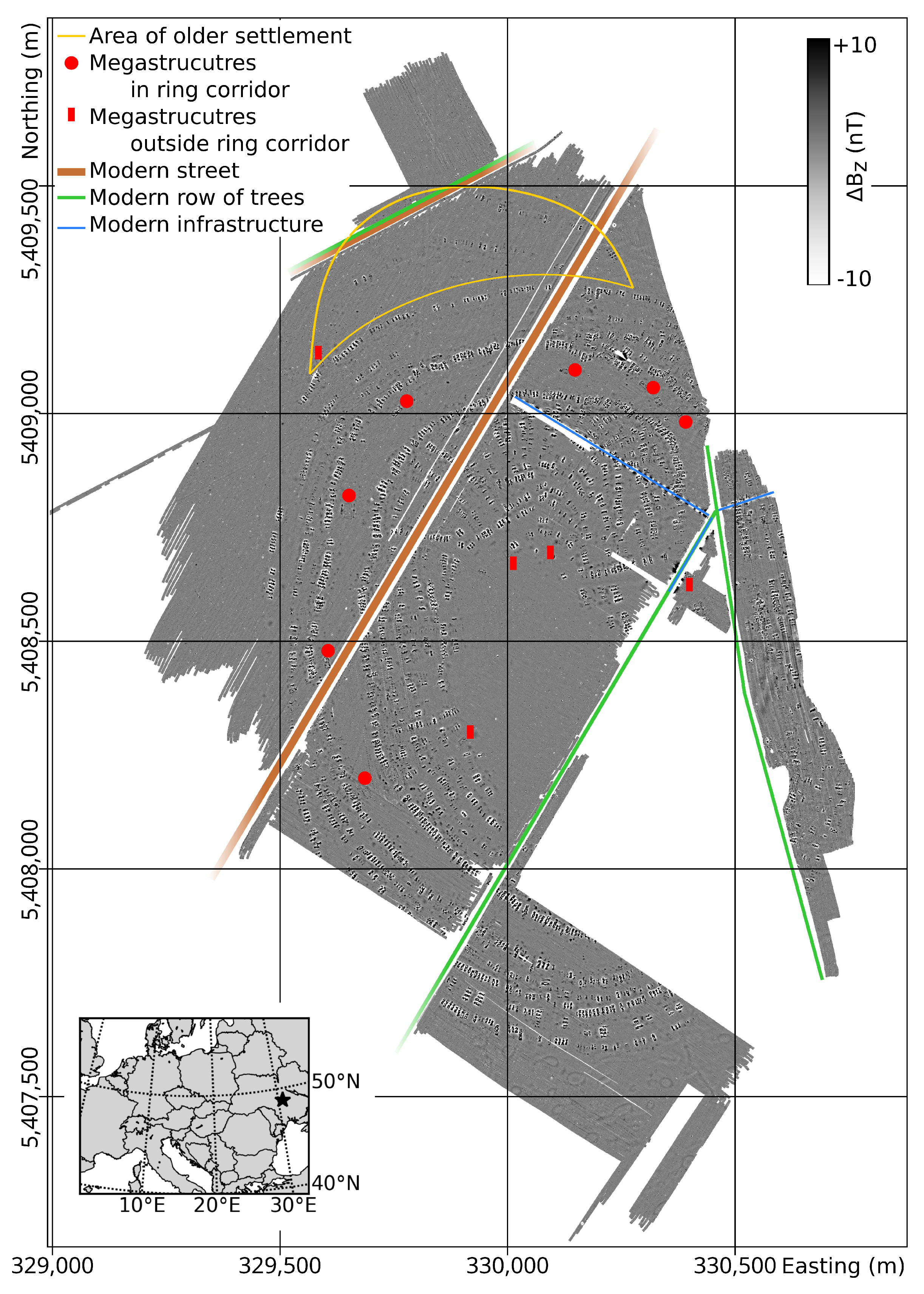
Magnetic map of the Maidanetske site (data kindly provided by the Romano-Germanic Commission, German Archaeological Institute, and Institute of Prehistoric and Protohistoric Archaeology, Kiel University; projection: UTM 36N). The locations of megastructures inside the ring corridor are marked with red circles, the remaining ones with red blocks. Moreover, the area of the older settlement phase is outlined in yellow. The measured area is interrupted by a modern street (brown), infrastructure (blue), and rows of trees (green).
2. Materials and Methods
First, we present the extensive magnetic map of Maidanetske [15,17] as the base material we use in the interpretation scheme. The interpretation scheme consists of two parts presented in the following sections: (1) the derivation of the magnetization distribution by inverse filtering and (2) the quantification of the buildings using the magnetization distribution.
2.1. Magnetic Data
In 2011 and 2012 the site was surveyed by the Romano-Germanic Commission of the German Archaeological Institute with a 16-gradiometer array by Sensys [18]. The gradiometers (FGM650) have a distance of 25 cm between each other in the array and are mounted 35 cm above the ground. The distance between the lower and upper sensor is 65 cm. In 2016, additional surveys by the Institute of Prehistoric and Protohistoric Archaeology, Kiel University were conducted with an 8-sensor array with a 50 cm sensor distance. While the smaller array was moved by foot, the larger one was pulled by a four-wheel drive vehicle.
Before the inverse filtering, the magnetic data were preprocessed with the following steps: subtraction of the median from each sensor trace, gridding onto a regular 0.25 m × 0.25 m grid and subtraction of the 2D median with a kernel size of 75 × 75 grid cells from the central cell. The first processing step eliminates sensor offsets. The second one reduces the regional and large-scale magnetic anomalies, respectively, and constitutes the main difference in processing compared to previously published versions of the magnetic map [15,17].
About 2300 house remains are visible in the magnetic map (Figure 1). The magnetic anomalies of the burned buildings are arranged along concentric ellipses around an inner vacant space. A corridor, which is free of houses, divides the settlement into an inner and outer part. The houses that are directly located along this corridor belong to the so-called “ring corridor”. Inside this free space are the megastructures, buildings with a different architecture than houses. North, outside of the outermost ellipse, remains of an older settlement are visible.
2.2. Inverse Filtering
Inversion filtering determines the magnetization distribution of magnetic prospection data for cases where an equivalent layer approach is applicable. For a site with a uniform magnetization direction and a consistent depth range of the magnetic source bodies, only one filter is needed. The basic idea [11,19,20,21,22] is as follows:
A horizontal layer is divided into a grid of blocks of equal size but different average magnetizations. The magnetic anomaly T of this layer can be written as a discrete 2D convolution of the magnetization distribution D and a kernel R:
where ∗ denotes convolution. is the magnetic anomaly in an observation plane parallel to the layer, is a matrix containing the magnetization values of the blocks and R represents the magnetic field of a block of unit magnetization in the observation plane (Green’s function). depends on the shape of the block (—extension in the east–west direction, —extension in the north–south direction, t—thickness/height, d—depth below surface to the top), the direction of magnetization (—inclination, —declination) and the distance of the observation plane from the magnetized layer (—heights of gradiometer sensors). T, D, and R are in matrix form. Following Equation (1), T can be understood as the output of a digital linear 2D filter R applied to a given magnetization distribution D (cf. Figure 2). Inversely, if the magnetic field T is given, the unknown magnetization distribution D can be determined from T by convolving the field T with an inverse filter operator :
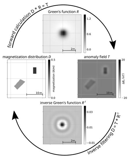
Figure 2.
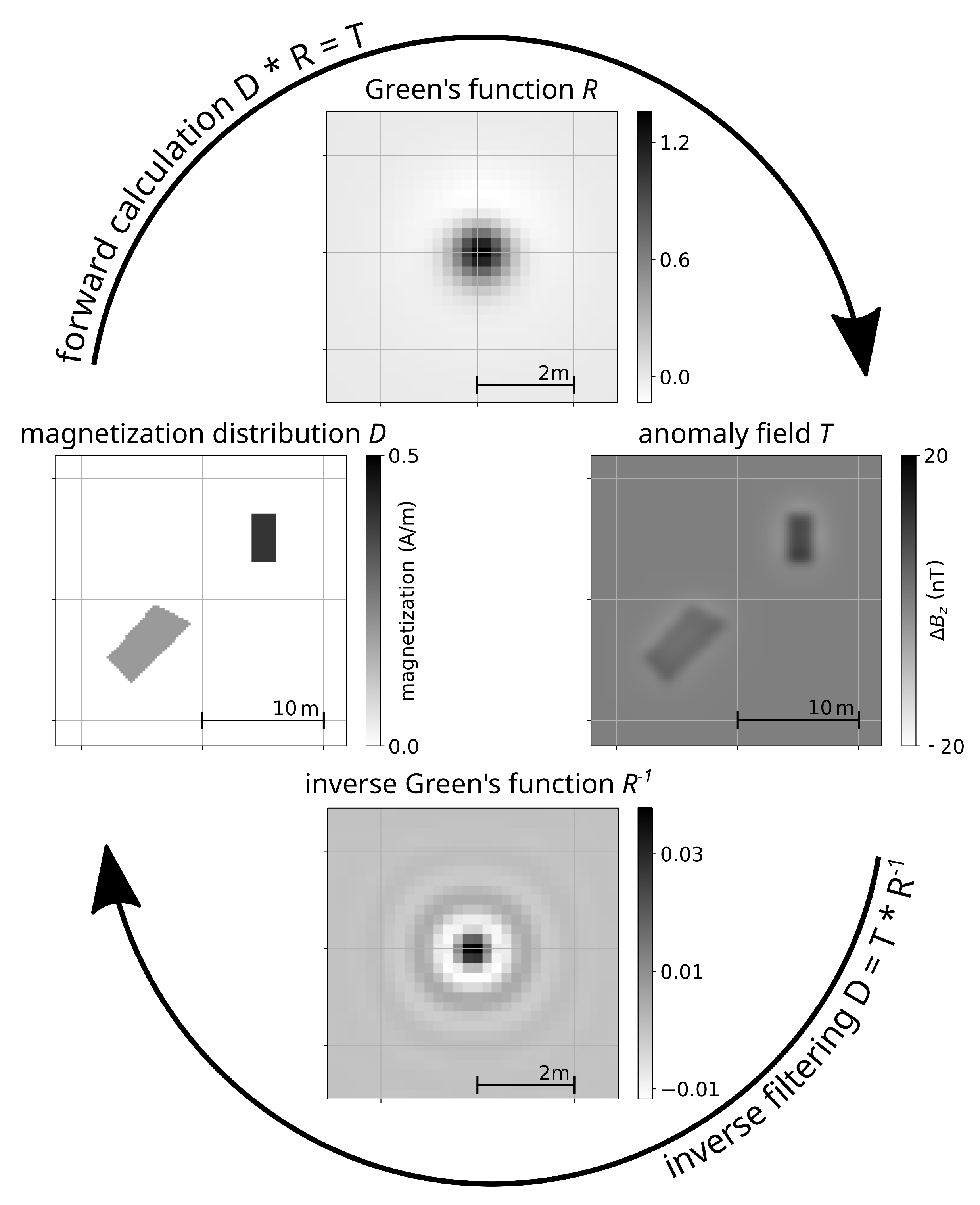
Illustration of methodical concept. The magnetization distribution D and the magnetic anomaly field T are related by the Green’s function R in terms of forward calculation and by the inverse of R in terms of inverse filtering.
The inverse matrix-form operator is determined from
where I is the unit element of convolution. I is a matrix, the elements of which are zero except for the central position of the matrix being 1. Since the number of elements of the involved matrices can only be finite, we can only determine the truncated version of the ideally infinitely wide through the minimization of
We calculated R with the Python library “Fatiando a Terra” [23] based on the formula for uniformly magnetized prisms [24]. The minimization of Equation (4) was performed with a least-squares solver in Python (scipy.optimize.least_squares). To ensure a stable minimization result for , smoothness constraints for the elements in this matrix were introduced. For this purpose, the difference between each cell to its four nearest neighbors was also minimized.
Figure 2 illustrates the above-described concept. The magnetization distribution D and the magnetic anomaly field T are linked through the kernel function R or its inverse . In the first case, this linkage is the forward calculation following Equation (1) (Figure 2, upper part) or, in the latter case, the inverse filtering following Equation (2) (Figure 2, lower part).
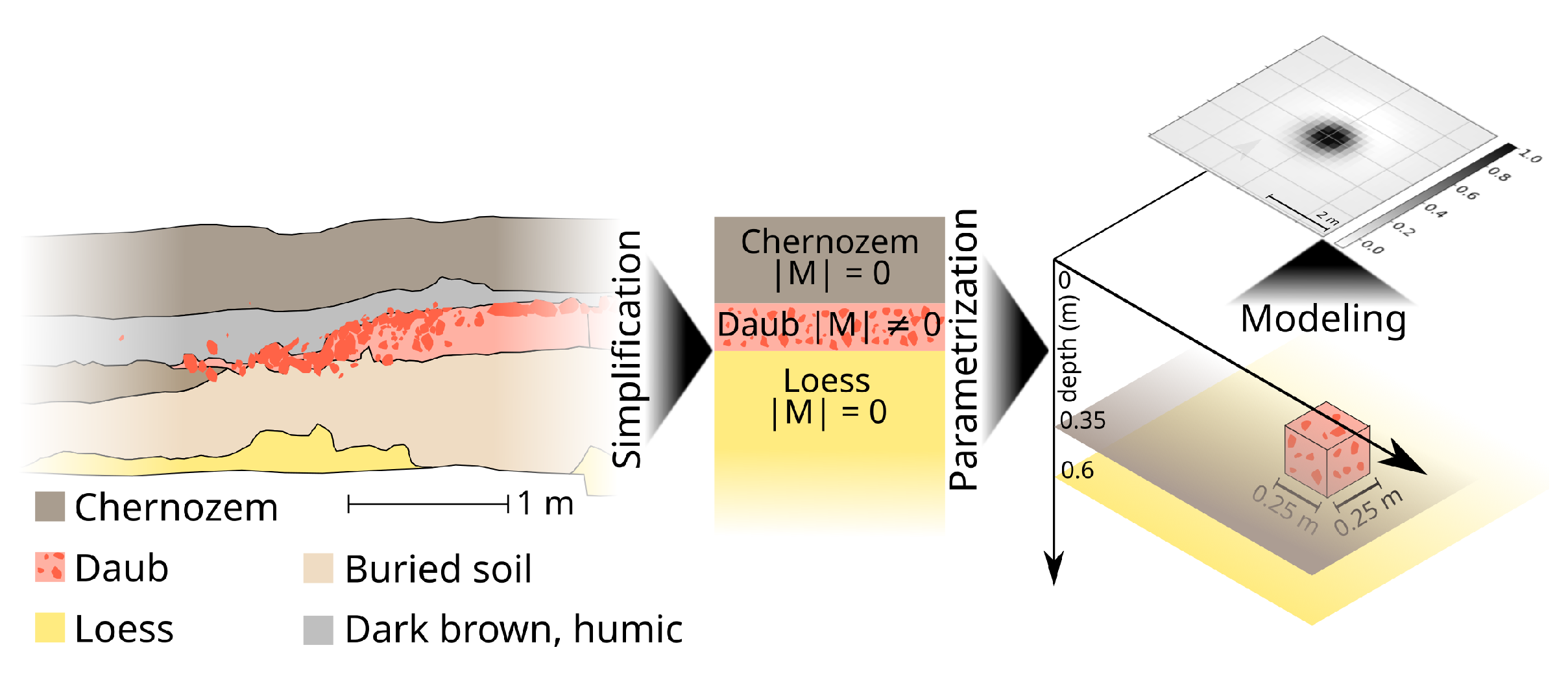
Figure 3 depicts the determination of the Green’s function R using an excavated archaeological section, alternatively, the section drilled cores can be used. The archaeological section consists of several (archaeological) layers, including the daub layer of the house remains (Figure 3, left). The daub layer is buried beneath chernozem and lies on a buried soil and loess. The archaeological section is simplified to a three-layer case composed of chernozem (top), daub (middle), and loess (bottom) (Figure 3, center). It was shown that the daub is the main magnetic source body [12] and therefore, we neglected the magnetization of the top and bottom layer (fixed to zero). Moreover, the influence of regional magnetization variations were removed by the median filters (cf. Section 2.1). Therefore, only in the depth range of the daub layer was a non-zero magnetization allowed and this determined the depth range of the filter. The magnetized block was parametrized with the values listed in Table 1 and R was calculated by forward modeling. R is the Green’s function of a magnetized block (Figure 3, right) in the target’s depth range.

Figure 3.
Schematic pathway from the archaeological section (left, after Figure 15 in [16] ) to the Green’s function R via simplification, parametrization, and modeling. Reproduced with permission from Robert Hofmann, Maidanetske 2013: New Excavations at a Trypilia Mega-Site; published by Dr. Rudolf Habelt GmbH, 2017.

Table 1.
Parameters and their values for filters A and B.
Table 1 distinguishes between filter A, which is used for the synthetic test (cf. Section 2.4) and the field example (cf. Section 3.1), and filter B, which is used for cross-checking with the least-squares inversion in Section 2.5. The parameters in Table 1 have the following origins: the target layer and the a priori information of its magnetization determine the depth and thickness of the block as well as the fixed orientation of the magnetization’s direction. With an assumed dominating portion of induced magnetization, the inclination and declination can be derived from the International Geomagnetic Reference Field (IGRF). Since the building remains are burned, we expect a high portion of remanent magnetization. The orientation of the remanent magnetization from collapsed daub buildings is highly variable based on the order of burning, collapsing, and cooling [25,26]. If the orientation is unambiguous, e.g., for kilns, a paleomagnetic field model can be used to determine the ancient orientation. We compared the values from the IGRF with values derived from the CALS10k-model [27]. For the settlement time of Maidanetske, the IGRF’s declination and inclination lie within the uncertainty range of the CALS10k-model. Hence, for burned material that remained in its in situ location of cooling down below the Curie point, the recent IGRF values are a good approximation. Therefore, we used the IGRF [28] values as listed in Table 1. The discretization depends on the measurement’s sample density as well as available computing power or time. Setting the magnetization of the block to 1 A/m resulted in a filter that directly generated the magnetization distribution.
The truncation length of the filter was determined based on the expected magnetization amplitude and the resolution of the magnetometer using an autocorrelation based on the approach presented by [22]: the filter is truncated at the distance where the autocorrelation of the filter is smaller than the squared resolution. This distance was determined for a magnetized block as parameterized in Table 1, except for its magnetization. To account for the larger area in which the magnetic field of a stronger magnetized body is detectable, we used the maximum expected magnetization instead of 1 A/m. We were expecting magnetization values up to 5 A/m [12]. Figure 4 compares for two magnetized blocks of 1 A/m or 5 A/m the autocorrelation of the maximum values of R with respect to the distance to the block. The horizontal line marks the threshold of 0.04 nT2, which is the squared resolution of the sensors as stated by the manufacturer [18]. For a magnetization of 1 A/m, the maximum value falls below 0.04 nT2 at 7 m, and for a magnetization of 5 A/m at 13 m away from the center. However, we also need to consider that increasing the filter area leads to increased magnetization values. In synthetic models with vanishing magnetization outside of the targets, this is not the case. When the surrounding material of the structure has zero magnetization the magnetic anomaly vanishes to zero at the respective distance from the source. However, in field examples, the magnetic field anomaly does—in general—not vanish and therefore the magnetization as a result of the inverse filtering increases with the filter size. We truncated R and therefore also after 12 m.
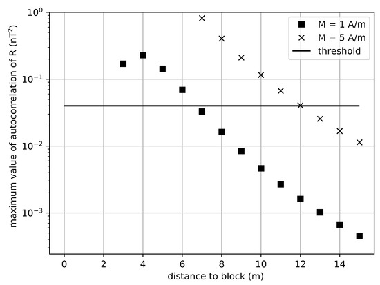
Figure 4.
Maximum value of the autocorrelation of R with increasing distance to the magnetized block with a magnetization of 1 A/m (squares) and 5 A/m (crosses). The distance to the block corresponds to the length of R. The horizontal line indicates the resolution of the sensors.
2.3. Quantification of Building Remains
With the above described assumptions, the magnetization distribution can be derived by inverse filtering and can thus build the base for quantifying building remains. The quantification in terms of magnetic moment constitutes a new database for inferring the social structure inside Cucuteni–Tripolye settlements.
The quantification of the buildings in terms of the magnetic moment is based on the visual interpretation of the magnetic map (Figure 24 in [15]). All anomalies interpreted as buildings were manually redrawn with polygons. These polygons were the starting point for the quantification. In order to refine the manually redrawn polygons more objectively based on the magnetization distribution, we determined a threshold on the magnetization distribution for detecting the edge of each building using the following approach. Since the magnetization outside of the buildings varies throughout the site—by, i.a., local soil composition and regional geological magnetic anomalies, as well as the effects of plowing—we determined the threshold for each building separately. We considered the magnetization values in a 1 m wide stripe outside around the manually drawn polygon and used the 75% percentile of these values as the threshold [12]. The 75% mark was derived based on a detailed consideration of completely excavated buildings. To quantify the buildings, we summed all magnetization values inside the polygon that were above the buildings specific threshold and multiplied the sum of the magnetization values with the volume of the block for constructing the filter. For all buildings, this yielded their magnetic moment in polygon j with . Lastly, the grid cells with magnetization values above the threshold were used to construct the minimum area rectangle to determine the ground plan area. Moreover, the minimum area rectangle yielded width and length as well as rotation angle of the buildings. These five parameters—magnetic moment, ground plan area, width, length, rotation angle—build the new data base derived from the magnetic map to infer social structures within the settlement or even comparisons across settlements.
Before turning to tests and modeling studies with the inverse filter approach, we note the choice of the color map for the derived magnetization distributions with respect to the expected value range. We chose to display the calculated magnetization distributions with a red-white-gray color map, where the red part covers the negative amplitudes of the magnetization. As a vector field, the magnetization can be oriented opposite the magnetic field strength for diamagnetic materials. Here, we mapped the magnetization intensity in the direction of the orientation that we fixed when calculating the filters (cf. Table 1). Since we were not expecting any purely diamagnetic bodies in the equivalent layer depth range, negative magnetization values resulted from a mismatch between the applied filter and the actual subsurface conditions. For field data, this was, apart from the orientation, a mismatch between the depth ranges which applies to surface clutter and deeper, geological structures.
Next, we provide a test on modeled data. Second, we compare the magnetization distribution derived by the least-squares approach [12] and by the inverse filtering on a field example. Furthermore, before turning to the results of the field data, we examine the influence of depth and thickness of the filter layer on a reference model.
2.4. Synthetic Test
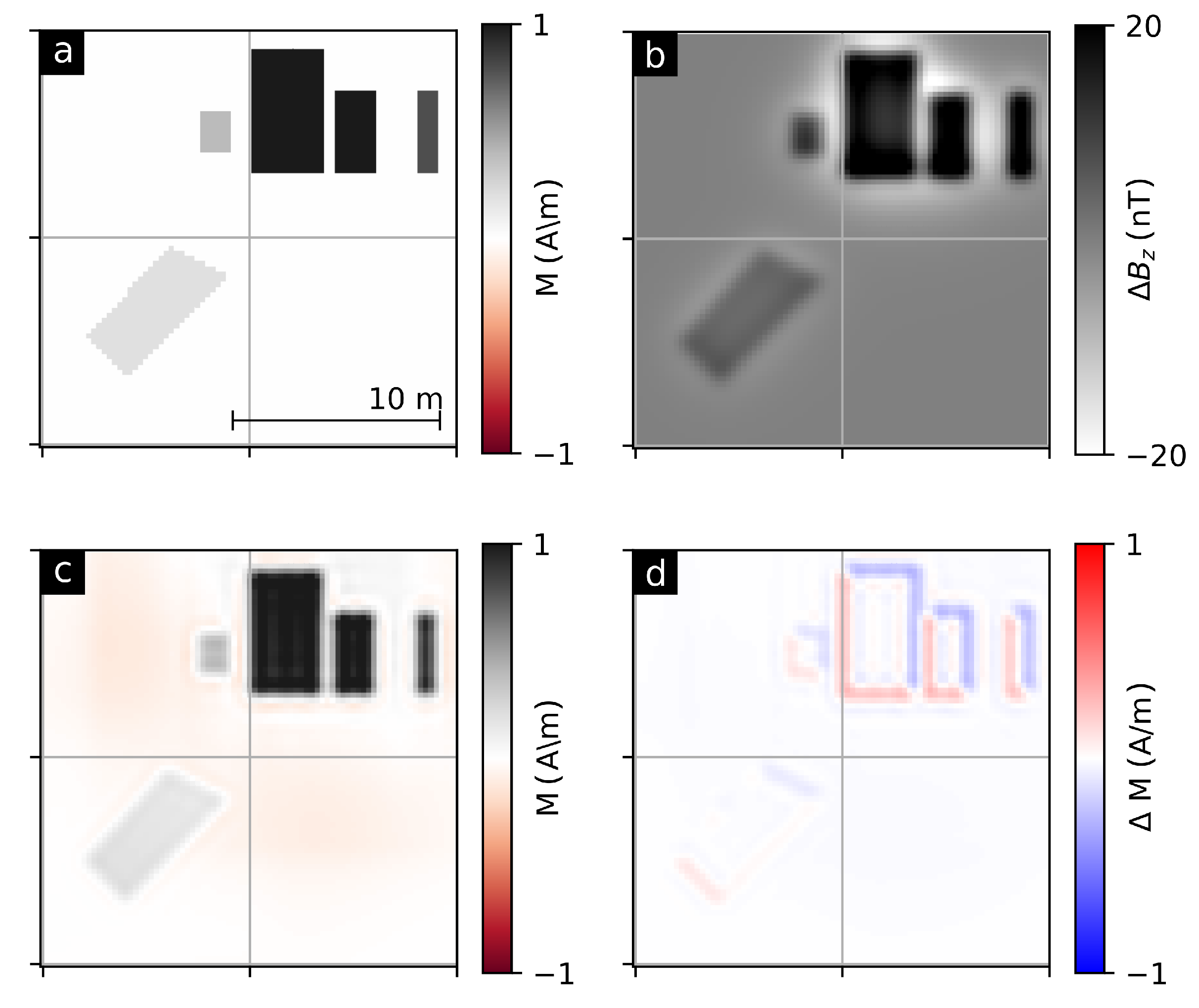
To test the accuracy and resolution of the inversion, we applied the filter on modeled data resembling the field example. Figure 5a shows the magnetization model that represents the remains of burnt clay houses at 0.35 m to 0.6 m depth with varying magnetization amplitudes. All other parameters are set to the values of filter A (Table 1) for both the model and the filter. The only exception is the length of the filter. As the maximum magnetization of the buildings was set to 1 A/m, the filter length was set to 8 m. The magnetization distribution derived by inverse filtering is presented in Figure 5c. Comparing the original model and the inversion result, only slight differences along the borders of the magnetized bodies are visible, as shown in Figure 5d. This test provides convincing evidence demonstrating that inverse filtering is a suitable method to determine the magnetization distribution of archaeological structures in a distinct depth range.

Figure 5.
Synthetic case study: (a) magnetization distribution at depth range 0.35 m to 0.6 m. (b) Resulting gradiometry data of (a). (c) Magnetization distribution derived from (b) via inverse filtering. (d) Deviation between (a) and (c).
2.5. Comparison to Least-Squares Inversion
We compare the magnetization distributions derived from the least-squares inversion and from the inverse filtering on the example of a so-called megastructure. The magnetization distribution based on the least-squares inversion as well as its methodological details were presented in [12]. For the least-squares inversion, the same assumptions as here were made: an equivalent layer approach with a fixed direction of magnetization based on the IGRF. The optimization was performed on a regular grid with smoothness constraints and allowing only positive magnetization values. For a direct comparison of both inversion approaches, we computed a filter with the same parameters that were used for the least-squares inversion. They are listed in Table 1 for filter B. Based on the least-squares inversion, we were expecting magnetization values up to 1.72 A/m. The argumentation based on the autocorrelation indicated a filter length of 10 m for a maximum magnetization up to 2 A/m in the depth range of this building.
Figure 6 shows the magnetic map (a), the magnetization distribution derived from the inverse filtering (b), the magnetization distribution derived from the least-squares inversion (c), and the deviation between the two latter ones (d). Both inversion approaches derive magnetization distributions that are consistent with each other. The maximum deviations between the two are in the order of ±0.5 A/m and coincide with the location of the megastructure. However, the layout of the building is not visible in the deviations. Hence, the main part of the magnetic anomaly is explained by both derived magnetization distributions in the same manner.
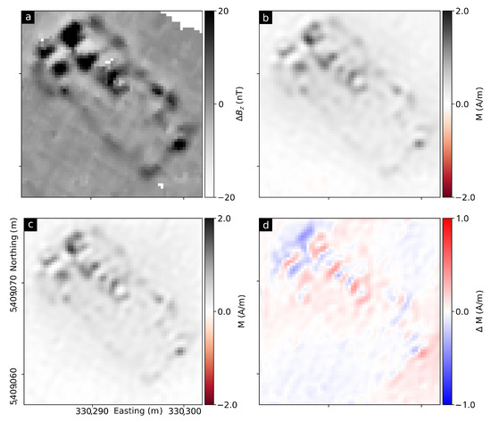
Figure 6.
Comparison of magnetization distributions derived with least-squares inversion (c) and inverse filtering (b) on the example of a megastructure (magnetic map—a) and difference between the two magnetization distributions (d).
The synthetic test (Section 2.4) as well as the comparison of both inversion approaches demonstrate that the inverse filtering provides reasonable magnetization distributions for the following case study.
2.6. Influence of Depth and Thickness
The depth and thickness of the magnetized layer are two crucial parameters for the construction of the filter. Yet, they might vary throughout the site or even on a smaller scale throughout one building. Depth and thickness can be inferred by other geophysical methods such as ground-penetrating radar, electromagnetic induction measurements, or electrical resistivity tomography, if the examined physical property changes accordingly to the magnetization. Another possibility is to derive them from excavations or drillings.
To assess the variability of depth and thickness of the daub layer within one building, these two parameters were measured along the excavated, latitudinal profile through house 44 (Figure 15 in [16]). The thickness varied between 0.05 m and 0.35 m with a mean thickness of 0.25 m and the depth between 0.5 m and 0.85 m. The evaluation of geoarchaeological depth profiles within excavations showed that the depth of the daub layer varied between 0.25 m and 0.5 m in between buildings with a mean depth of 0.35 m.
To make deviations in depth and thickness between the subsurface conditions and the applied filter tangible, we conducted a modeling study for varying depth and thickness values in the filter construction for one fixed reference model (“the true subsurface conditions”). The reference model is shown in Figure 2 as the magnetization distribution D. The only difference with the reference model is a reduced resolution with increased discretization step from 0.25 m to 0.5 m to reduce computation time. The magnetized layer is located at a 0.35 m depth with a thickness of 0.25 m, based on the excavations.
The assumed filters are constructed based on the parameters shown in Table 1—Filter A, with m with varying depth and thickness values. The depth of the magnetized layer was varied from 0.00 m to 1.00 m in 0.05 m steps and its thickness from 0.05 m to 1.00 m also in 0.05 m steps. Therefore, we derived 420 different filters ,which were each applied to the magnetic field data based on the reference model. The resulting inverse filtering results were then compared to the reference model as shown in Figure 7 and Figure 8.
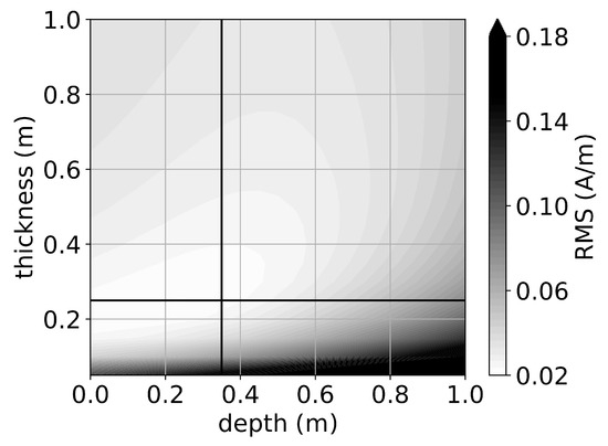
Figure 7.
Root mean square (RMS) error between reference model and inverse filtering results for varying depth and thickness values of the layer in the filter. The black lines mark the correct values for depth (0.35 m) and thickness (0.25 m).
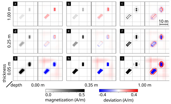
Figure 8.
Magnetization distribution (each left one) derived by inverse filtering and its deviation to the reference model (each right one) for nine different filters with different depth d and thickness t combinations: (a) d: 0.00 m, t: 1.00 m; (b) d: 0.35 m, t: 1.00 m; (c) d: 1.00 m, t: 1.00 m; (d) d: 0.00 m, t: 0.25 m; (e) d: 0.35 m, t: 0.25 m; (f) d: 1.00 m, t: 0.25 m; (g) d: 0.00 m, t: 0.05 m; (h) d: 0.35 m, t: 0.05 m; (i) d: 1.00 m, t: 0.05 m.
Figure 7 depicts the root mean square (RMS) error between the reference model and the inverse filtering results for varying depth and thickness values. The black lines mark the correct values of depth and thickness of the synthetic reference model. Different assumed combinations of depth (0.00 m to 0.45 m) and thickness (0.15 m to 0.40 m) lead to the smallest values of the RMS error (approximately 0.02 A/m). In our synthetic example, a 0.02 A/m deviation from the maximum magnetization translates to 5%. The highest RMS errors occur when the thickness of the layer is assumed to be too small.
Figure 8 shows nine different inverse filtering results and the deviation to the reference model. The results for the filter in accordance with the reference model is shown in the center (e: depth = 0.35 m; thickness = 0.25 m). In this case, the inverse filtering results deviate at the borders of the magnetized blocks. For a thickness assumed to be too small, the magnetization is overrated by inverse filtering (Figure 8g–i). Vice versa, the magnetization is underrated by inverse filtering for too large a thickness (Figure 8a–c). When the depth of the assumed layer is too close to the surface, the borders of the magnetized body are blurred (Figure 8a,d,g). When the assumed depth is deeper than the actual layer, a magnetized area appears as corona in a few meters of distance to the actual magnetized body (Figure 8c,f,i). For thinner thicknesses, the deviation shows artifacts from the border of the model area.
3. Results of Maidanetske
In this section, we present the magnetization distribution derived by inverse filtering for the complete survey area and inspect a subarea in detail. Finally, we give an overview of the quantification.
3.1. Magnetization Distribution
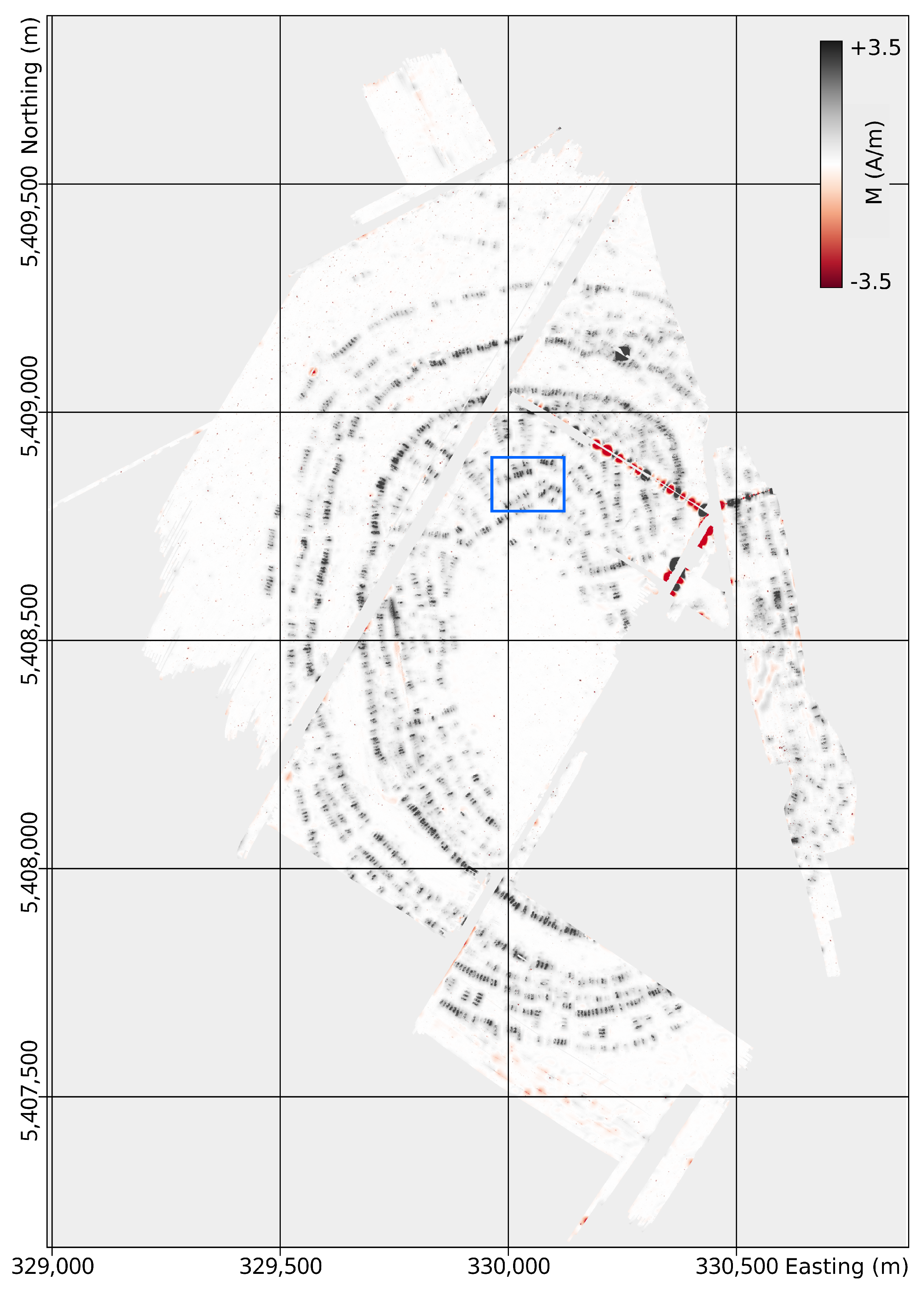
Figure 9 shows the magnetization distribution derived by inverse filtering for the complete site. The locations of the buildings are marked by increased magnetization values. Besides those anomalies, anomalies from infrastructures are visible in the northeastern part of the site (cf. Figure 1, blue lines), which can be ignored in the further interpretation. In the east, variations at a local scale indicate the locations of regional, geological structures.
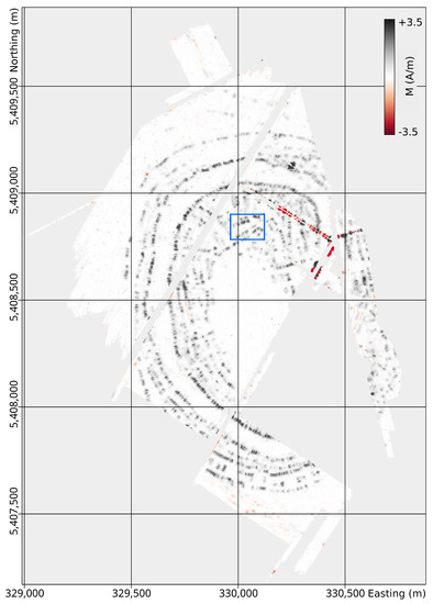
Figure 9.
Magnetization distribution of Maidanetske derived by inverse filtering. The blue box marks the area shown in Figure 10.
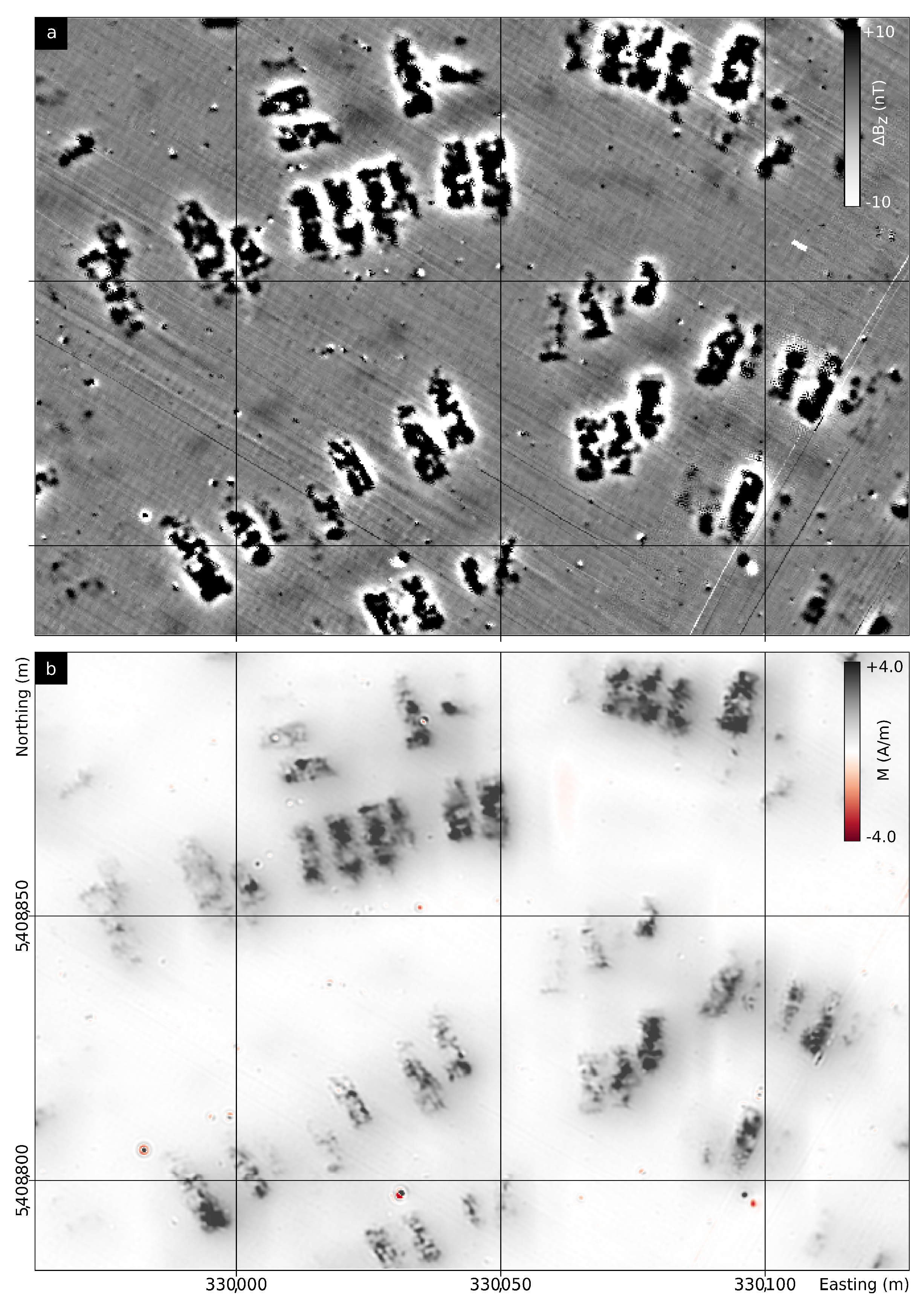
To discuss the magnetization distributions of the buildings in detail, we show in Figure 10 a smaller area (cf. Figure 9, blue box). In this subarea are buildings of different sizes and with different magnetization patterns and amplitudes. Moreover, the buildings vary in their ratio of length to width. The comparison between the magnetic map (Figure 10a) and the magnetization distribution highlights the difference of the anomaly field to the magnetic property distribution. While the anomalies in the magnetic map are clearly dipolar, the magnetization distribution is non-dipolar. Increased magnetization values display the location and extent of the magnetic source bodies. Consequently, the magnetization patterns indicate the distribution of daub [12] and subsequently the ground floor plan or architecture of each building. Since the amplitude of the magnetization is related to the mass of remaining daub in the subsurface [12], the magnetization distribution indicates buildings with high and low amount of daub by high and low magnetization values. Therefore, the magnetization map enables a finer differentiation of buildings with respect to the amount of daub. To quantify this differentiation, we derived the magnetic moment for each building.
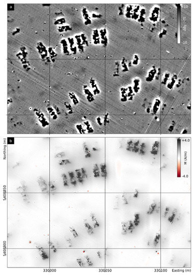
Figure 10.
Comparison of the magnetic map (a) and the magnetization distribution (b) for a subarea of the site with several anomalies of burnt buildings. The location of this subarea is marked in Figure 9 with a blue box.
3.2. Quantification Results
The magnetic moments for all buildings are shown in Figure 11. The highest values (m > 60 Am2) of the magnetic moments are predominantly located along the ring corridor, especially along the inner ring and in the south of the settlement. On the contrary, the magnetic moments of the buildings belonging to the older settlement in the north are low (m < 30 Am2).
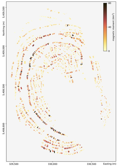
Figure 11.
Magnetic moment of each building derived from the magnetization distribution.
4. Discussion
To infer the social structure of archaeological sites, we presented an interpretation scheme based on magnetic prospection data. This scheme comprised two steps: first, deriving the magnetization distribution for the complete site via inverse filtering and second, quantifying the archaeological structures in terms of their magnetic moment. Focusing on the methodical aspects, the tests on synthetic data and the comparison of the two inversion results derived by inverse filtering and the least-squares approach [12] provided convincing evidence that the magnetization distribution was reliable.
Compared to the least-squares approach, inverse filtering had two advantages in terms of feasibility. For the least-squares inversion, it was necessary to cut out each building so that the computations could be performed on a standard desktop machine. This also involved one (time-expensive) inversion computation for each building. For the inverse filtering approach, only one inversion for the construction of the filter was needed. The magnetization distribution for the complete area was then derived by a convolution, which was a faster computational step.
Concerning the applicability of this approach to other sites, the choice of depth and thickness for the magnetized layer for the filter construction might be related to the highest inaccuracies, as depth and thickness may vary throughout the site and even throughout each building. We established the following qualitative guideline based on the RMS error distribution and the deviation patterns in the modeling study (cf. Section 2.6): (1) It is better to choose a layer too thick than too thin (reason: in the modeling study, the RMS error rose quicker with layers too thin). (2) It is better to choose a layer too deep than too shallow (reason: in the modeling study, the RMS error rose quicker with layers closer to the surface). (3) Small variations in depth and thickness do not affect the inverse filtering result significantly (reason: several combinations of depth and thickness for the filter layer yielded similar inverse filtering results in terms of the RMS error. This illustrates the inherent ambiguity of potential field data). (4) Blurred borders in the magnetization distribution derived by inverse filtering might indicate a filter layer too close to the surface (reason: the magnetization patterns (Figure 8) indicated this. This only applies to bodies with expected sharp borders in the magnetization distribution). (5) Magnetized coronas around magnetized areas might indicate a filter layer that is deeper than the actual layer (reason and limitation as in point 4).
For Maidanetske, the depth range of the daub layer is known from excavations and test trenches for 23 buildings. The top of the daub layer starts at an average depth of 35 cm and has an average thickness of 25 cm. Depth and thickness of the daub layer vary throughout the site and even throughout each building. The variation of the top layers thickness throughout the site may result from different cultivation of the fields or effects of erosion along the slopes. Moreover, the variation of the daub layers thickness throughout the site and each building could be due to different construction elements, burning conditions, and state of preservation. The direct determination of depth and thickness of the daub layer via excavations, corings, or additional geophysical measurements is expensive in terms of time and cost, and therefore not feasible on a broad scale. Since the currently available depth data from excavations show only small variations, the application of a constant depth range for inverse filtering is permissible. This simplification is also supported by the modeling study, as it showed that different combinations of depth and thickness lead to similar fits in terms of the RMS error. For further applications, the magnetic map can be divided into areas for which a constant depth range approximation holds and a respective filter can be applied to the subareas, if considerable depth variations are present at a site.
The quantification of the buildings in terms of total magnetization, ground floor area, length, and width depends on the manual interpretation of the magnetic map as it is based on the polygons. The determination of a threshold based on the data objectifies this quantification compared to manual interpretation. If the manually drawn polygons underestimate the area for a building, the threshold approach does not allow an increase of the initial area. However, the skewness and dipolar character of magnetic anomalies rather lead to an overestimation of building areas. Further improvements could be made by implementing an automatic object detection.
The magnetization distribution is the basis for determining the magnetic moment, the ground floor area, and the pattern of magnetization for each building. Previously, we have shown that the magnetization pattern is related to the standardized floor plans of the Tripolye houses and that, per excavation grid, the mean magnetization is correlated with the mass of the remaining daub [12]. Hence, the magnetic moment serves as a proxy for the total mass of remaining daub for each building. Based on the assumption that the architecture and amount of building material reflects economic and social power of the bygone inhabitants, the magnetization distribution is an ideal base to infer the social structure. A detailed interpretation of the total magnetization, ground floor area, width and length of the buildings is beyond the scope of this methodically focused paper and will follow in a further publication.
5. Conclusions
We presented an interpretation scheme, consisting of inverse filtering, to derive the magnetization distribution and the quantification of the buildings in terms of their total magnetization. The magnetization patterns indicated the ground floor plans. Moreover, the distribution of the magnetic moment, as a proxy for the mass of building material, provided convincing evidence demonstrating that the magnetic moment is related to the social structure at the Cucuteni–Tripolye site, Maidanetske. Hence, the calculation of the underlying magnetization distribution yields new data to infer the social structure of sites.
With our modeling study, we provided a guideline to find out if the depth and thickness of the layer for filter construction is chosen adequately. It is better to choose a layer that is too deep and too thick, than one that is too shallow and too thin. There is a range of depth and thickness combinations that produces equivalently good magnetization distributions. Coronas around magnetized areas might indicate a depth that is significantly too deep, and blurred borders of magnetized areas might indicate a depth that is significantly too low.
Finally, inverse filtering provides a fast computation of the magnetization distribution for objects that can be represented by an equivalent layer. The magnetization distribution has several advantages compared to the magnetic field data: it is a better database to delineate the size of objects, it represents the find distribution, and yields a gateway to the social structure.
Author Contributions
Conceptualization, N.P. and W.R.; methodology, N.P.; software, N.P.; validation, N.P. and T.W.; investigation, K.R., R.H. and R.O.; writing—original draft preparation, N.P.; writing—review and editing, N.P., T.W., W.R., D.W. and M.T.; visualization, N.P.; supervision, W.R.; funding acquisition, D.W., T.W., W.R. and J.M.; project administration, M.V. and J.M. All authors have read and agreed to the published version of the manuscript.
Funding
The work was funded by the Deutsche Forschungsgemeinschaft (DFG, German Research Foundation)—Project-ID 290391021—Sonderforschungsbereich 1266.
Data Availability Statement
The data that support the findings of this study are available from the corresponding author upon reasonable request.
Acknowledgments
We thank two anonymous reviewers for their valuable comments that helped to improve the manuscript.
Conflicts of Interest
The authors declare no conflict of interest. The funders had no role in the design of the study; in the collection, analyses, or interpretation of data; in the writing of the manuscript, or in the decision to publish the results.
Abbreviations
The following abbreviations are used in this manuscript:
| IGRF | International Geomagnetic Reference Field |
| RMS | Root mean square |
References
- Eder-Hinterleitner, A.; Neubauer, W.; Melichar, P. Restoring magnetic anomalies. Archaeol. Prospect. 1996, 3, 13. [Google Scholar] [CrossRef]
- Blakely, R.J. Potential Theory in Gravity and Magnetic Applications; Cambridge University Press: Cambridge, UK, 1995. [Google Scholar]
- Eder-Hinterleitner, A.; Neubauer, W.; Melichar, P. Reconstruction of archaeological structures using magnetic prospection. Analecta Praehist. Leiden. 1996, 28, 131–137. [Google Scholar]
- Dittrich, G.; Koppelt, U. Quantitative interpretation of magnetic data over settlement structures by inverse modelling. Archaeol. Prospect. 1997, 4, 165–177. [Google Scholar] [CrossRef]
- Herwanger, J.; Maurer, H.; Green, A.G.; Leckebusch, J. 3-D inversions of magnetic gradiometer data in archeological prospecting: Possibilities and limitations. Geophysics 2000, 65, 849–860. [Google Scholar] [CrossRef]
- Li, Y.; Oldenburg, D.W. 3-D inversion of magnetic data. Geophysics 1996, 61, 394–408. [Google Scholar] [CrossRef]
- Bescoby, D.J.; Cawley, G.C.; Chroston, P.N. Enhanced interpretation of magnetic survey data from archaeological sites using artificial neural networks. Geophysics 2006, 71, H45–H53. [Google Scholar] [CrossRef]
- Schneider, M.; Stolz, R.; Linzen, S.; Schiffler, M.; Chwala, A.; Schulz, M.; Dunkel, S.; Meyer, H.G. Inversion of geo-magnetic full-tensor gradiometer data. J. Appl. Geophys. 2013, 92, 57–67. [Google Scholar] [CrossRef]
- Schneider, M.; Linzen, S.; Schiffler, M.; Pohl, E.; Ahrens, B.; Dunkel, S.; Stolz, R.; Bemmann, J.; Meyer, H.G.; Baumgarten, D. Inversion of Geo-Magnetic SQUID Gradiometer Prospection Data Using Polyhedral Model Interpretation of Elongated Anomalies. IEEE Trans. Magn. 2014, 50, 1–4. [Google Scholar] [CrossRef]
- Cheyney, S.; Fishwick, S.; Hill, I.; Linford, N. Successful adaptation of three-dimensional inversion methodologies for archaeological-scale, total-field magnetic data sets. Geophys. J. Int. 2015, 202, 1271–1288. [Google Scholar] [CrossRef] [Green Version]
- Tassis, G.; Hansen, R.; Tsokas, G.; Papazachos, C.; Tsourlos, P. Two-dimensional inverse filtering for the rectification of the magnetic gradiometry signal. Surf. Geophys. 2008, 6, 113–122. [Google Scholar] [CrossRef] [Green Version]
- Pickartz, N.; Hofmann, R.; Dreibrodt, S.; Rassmann, K.; Shatilo, L.; Ohlrau, R.; Wilken, D.; Rabbel, W. Deciphering archeological contexts from the magnetic map: Determination of daub distribution and mass of Chalcolithic house remains. Holocene 2019, 29, 1637–1652. [Google Scholar] [CrossRef]
- Chernovol, D. Houses of the Tomashovskaya local group. In The Tripolye Culture Giant-Settlements in Ukraine: Formation, Development and Decline; Menotti, F., Korvin-Piotrovskiy, A., Eds.; Oxbow Books: Oxford, UK, 2012. [Google Scholar]
- Kohler, T.A.; Smith, M.E.; Bogaard, A.; Feinman, G.M.; Peterson, C.E.; Betzenhauser, A.; Pailes, M.; Stone, E.C.; Marie Prentiss, A.; Dennehy, T.J.; et al. Greater post-Neolithic wealth disparities in Eurasia than in North America and Mesoamerica. Nature 2017, 551, 619–622. [Google Scholar] [CrossRef] [PubMed] [Green Version]
- Ohlrau, R. Maidanets’ke: Development and Decline of a Trypillia Mega-Site in Central Ukraine; Scales of Transformation in Prehistoric and Archaic Societies; Sidestone Press: Leiden, The Netherlands, 2020. [Google Scholar]
- Müller, J.; Hofmann, R.; Kirleis, W.; Dreibrodt, S.; Ohlrau, R.; Brandstätter, L.; Dal Corso, M.; Out, W.; Rassmann, K.; Burdo, N.; et al. Maidanetske 2013: New Excavations at a Trypilia Mega-Site; Dr. Rudolf Habelt GmbH: Bonn, Germany, 2017. [Google Scholar]
- Rassmann, K.; Ohlrau, R.; Hofmann, R.; Mischka, C.; Burdo, N.; Videjko, M.Y.; Müller, J. High precision Tripolye settlement plans, demographic estimations and settlement organization. J. Neolit. Archaeol. 2014, 96–134. [Google Scholar] [CrossRef]
- Sensys GmbH. FGM650 Gradiometer. Available online: https://sensysmagnetometer.com/products/fgm650-gradiometer/ (accessed on 26 December 2021).
- Papazachos, C.; Tsokas, G. A FORTRAN program for the computation of 2-dimensional inverse filters in magnetic prospecting. Comput. Geosci. 1993, 19, 705–715. [Google Scholar] [CrossRef]
- Tsokas, G.N.; Papazachos, C.B. The Applicability of Two-dimensional Inversion Filters in Magnetic Prospecting for Buried Antiquities. In Theory and Practice of Geophysical Data Inversion; Vogel, A., Sarwar, A.K.M., Gorenflo, R., Kounchev, O.I., Eds.; Vieweg+Teubner Verlag: Wiesbaden, Germany, 1992; pp. 121–144. [Google Scholar] [CrossRef]
- Tsokas, G.N.; Papazachos, C.B. Two-dimensional inversion filters in magnetic prospecting: Application to the exploration for buried antiquities. Geophysics 1992, 57, 1004–1013. [Google Scholar] [CrossRef] [Green Version]
- Tsokas, G.N.; Papazachos, C.B.; Loucoyannakis, M.Z.; Karousova, O. Geophysical data from archaeological sites: Inversion filters based on the vertical-sided finite prism model. Archaeometry 1991, 33, 215–230. [Google Scholar] [CrossRef]
- Uieda, L.; Oliveira, V.; Barbosa, V. Modeling the Earth with Fatiando a Terra. 2013. pp. 92–98. Available online: https://legacy.fatiando.org/cite.html#cite (accessed on 4 October 2021).
- Bhattacharyya, B.K. Magnetic anomalies due to prism-shaped bodies with arbitrary polarization. Geophysics 1964, 29, 517–531. [Google Scholar] [CrossRef]
- Shaffer, G.D. An Archaeomagnetic Study of a Wattle and Daub Building Collapse. J. Field Archaeol. 1993, 20, 59–75. [Google Scholar] [CrossRef]
- Wunderlich, T.; Kahn, R.; Nowaczyk, N.R.; Pickartz, N.; Schulte-Kortnack, D.; Hofmann, R.; Rabbel, W. On-site non-destructive determination of the remanent magnetization of archaeological finds using field magnetometers. Archaeol. Prospect. 2021, arp.1847. [Google Scholar] [CrossRef]
- Korte, M.; Constable, C.; Donadini, F.; Holme, R. Reconstructing the Holocene geomagnetic field. Earth Planet. Sci. Lett. 2011, 312, 497–505. [Google Scholar] [CrossRef] [Green Version]
- Magnetic Field Calculator. Available online: https://www.ngdc.noaa.gov/geomag/calculators/magcalc.shtm (accessed on 4 October 2021).


Publisher’s Note: MDPI stays neutral with regard to jurisdictional claims in published maps and institutional affiliations. |
© 2022 by the authors. Licensee MDPI, Basel, Switzerland. This article is an open access article distributed under the terms and conditions of the Creative Commons Attribution (CC BY) license (https://creativecommons.org/licenses/by/4.0/).