Small Sample Hyperspectral Image Classification Based on Cascade Fusion of Mixed Spatial-Spectral Features and Second-Order Pooling

Abstract

Hyperspectral images can capture subtle differences in reflectance of features in hundreds of narrow bands, and its pixel-wise classification is the cornerstone of many applications requiring fine-grained classification results. Although three-dimensional convolutional neural networks (3D-CNN) have been extensively investigated in hyperspectral image classification tasks and have made significant breakthroughs, hyperspectral classification under small sample conditions is still challenging. In order to facilitate small sample hyperspectral classification, a novel mixed spatial-spectral features cascade fusion network (MSSFN) is proposed. First, the covariance structure of hyperspectral data is modeled and dimensionality reduction is conducted using factor analysis. Then, two 3D spatial-spectral residual modules and one 2D separable spatial residual module are used to extract mixed spatial-spectral features. A cascade fusion pattern consisting of intra-block feature fusion and inter-block feature fusion is constructed to enhance the feature extraction capability. Finally, the second-order statistical information of the fused features is mined using second-order pooling and the classification is achieved by the fully connected layer after L2 normalization. On the three public available hyperspectral datasets, Indian Pines, Houston, and University of Pavia, only 5%, 3%, and 1% of the labeled samples were used for training, the accuracy of MSSFN in this paper is 98.52%, 96.31% and 98.83%, respectively, which is far better than the contrast models and verifies the effectiveness of MSSFN in small sample hyperspectral classification tasks.

1. Introduction

Hyperspectral images can capture subtle differences in reflectance of features in hundreds of narrow spectral bands, offering the possibility of accurate identification of features with comparable color and texture [1]. Therefore, hyperspectral image classification is the cornerstone of many applications requiring high classification granularity, such as agricultural yield estimation [2], tree species identification [3], natural resource survey [4], and disaster monitoring [5], and have long been a research hotspot in the field of remote sensing. Nowadays, deep learning methods represented by 3D-CNN are capable of automatically extracting joint spatial-spectral features, and have been extensively investigated and applied in hyperspectral remote sensing applications in recent years [6,7,8]. However, the raw hyperspectral data have a high redundancy, and it is difficult to obtain sufficient manually labeled samples [9]. The available training samples in real-world hyperspectral classification tasks are often scarce and contain considerable noise. Therefore, effective dimension reduction for hyperspectral images without losing crucial spatial-spectral features and achieving satisfactory classification accuracy with as few samples as possible is still very challenging [10,11].

Feature extraction and representation are key steps in hyperspectral image classification tasks [12,13]. Prior to the widespread applications of deep learning methods, hyperspectral classification relied on hand-crafted features. The shallow features extracted by such methods could not effectively handle complex situations with inter-class nuance and large intra-class variation, and the generalization ability to various datasets with variable spatial resolution and spectral signatures was insufficient [14,15]. Recently, deep learning methods have been extensively investigated in hyperspectral classification due to their capability of extracting deep hierarchical features from raw images in an end-to-end learning manner and the classification accuracy has been greatly boosted compared with traditional methods [16,17]. 2D-CNN and 3D-CNN are two commonly used methods for extracting spatial features and spatial-spectral features from pixels to be classified and their fixed neighborhood, respectively [18,19,20,21]. Although CNN models are currently the mainstream methods for hyperspectral classification, their black-box nature leads to a lack of clear connection between classification results and spectral physical significance. To this end, Makantasis et al. proposed a novel tensor-based learning method for hyperspectral data analysis, which significantly reduces the model parameter number and clearly interprets model coefficients on the classification results [22,23].

In order to improve the robustness of features learned by CNN models and accelerate network training, the residual learning method inspired by ResNet [24] is widely utilized for hyperspectral classification model construction. Lee et al. proposed Contextual CNN, which first learns contextual features through parallel $1\times 1$, $3\times 3$ and $5\times 5$ convolutional kernels, and then introduces residual learning in subsequent $1\times 1$ convolution sequences to improve classification accuracy [25]. Liu et al. 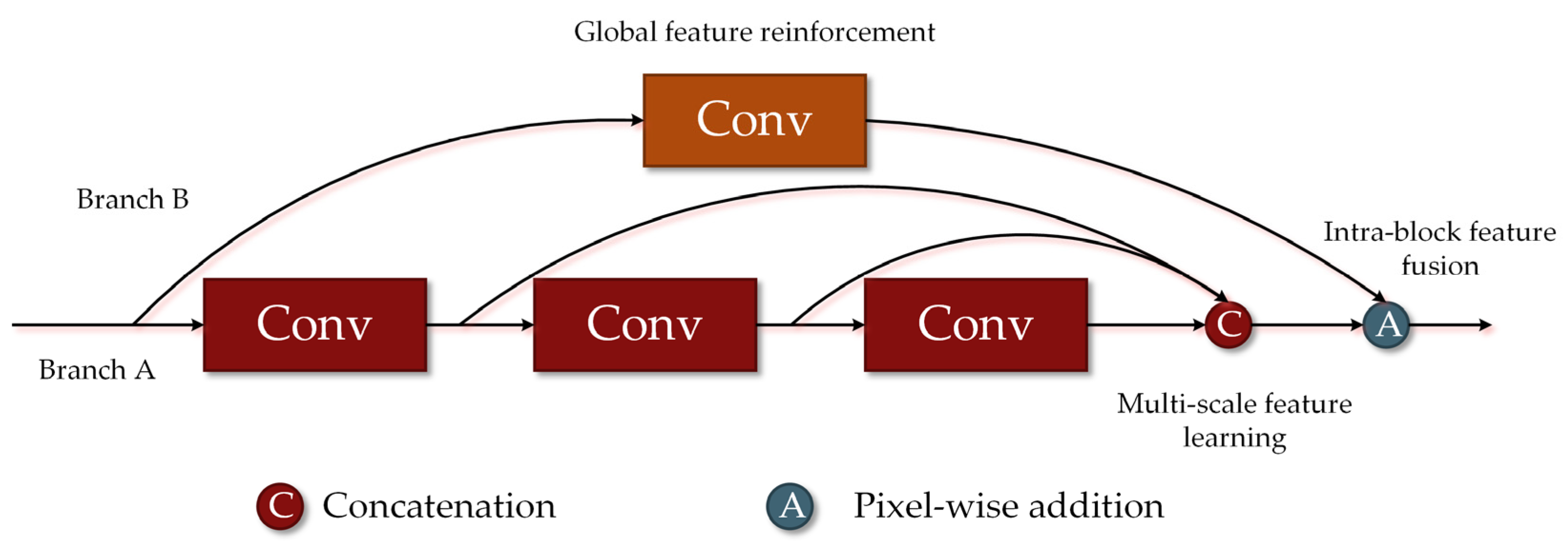introduced residual learning in a continuous 3D convolutional sequence and constructed a deep Res-3D-CNN to learn hierarchical spatial-spectral features, which improves classification accuracy compared to shallow 3D-CNN [26]. Song et al. proposed DFFN and deep residual learning was adopted to achieve intra-block feature fusion. The low-level, middle-level, and high-level features learned by different network parts were further fused to achieve inter-block feature fusion [27]. Dense connections, which was proposed by Huang et al., can be viewed as an extreme version of a residual connection that the output features of all the previous layers are concatenated and sent to the next layer for feature re-using [28]. Dense feature fusion patterns were then adopted to hyperspectral classification tasks and achieved success [29,30,31]. Residual learning and dense connectivity, which are served as the core approaches of feature fusion, have profoundly influenced the designed patterns of hyperspectral classification networks. However, the literature [32] indicated that frequent feature map concatenations based on existing deep learning frameworks could cause excessive memory consumption. Therefore, an effective and efficient feature learning pattern needs further investigation. Recently, attention-based spatial-spectral feature learning models for hyperspectral classification have gained enormous popularity and might be a solution to the above-mentioned feature learning problem [33,34,35].

Hyperspectral images are characterized by high dimensionality, and it is difficult to effectively filter redundancy when features are extracted with 3D-CNN under small sample conditions. In addition, to learn features from raw hyperspectral data, nested pooling layers are often required in 3D-CNN to reduce the feature map dimension and control the network parameter scale. However, the pre-defined pooling size may be detrimental to feature extraction. To address this problem, 3D-CNN and 2D-CNN are fused to extract spatial-spectral features from the down-scaled hyperspectral images. Roy et al. proposed HybridSN, which is a mixed 3D-2D-CNN model. The principal component analysis (PCA) was firstly adopted for down-scaling, and then the pipelined stacking 3D convolutional layers and 2D convolutional layers were used to extract spatial-spectral features, effectively improving the classification accuracy compared to networks with a single type of convolution [36]. Feng et al. proposed R-HybridSN based on residual learning and depth separable convolution, which effectively improved the obtained classification accuracy of hyperspectral images under small sample conditions [37]. Based on R-HybridSN, Feng et al. proposed M-HybridSN of which the core feature extraction module is a combination of three densely connected $3\times 3\times 3$ convolutional layers and one $7\times 7\times 7$ convolutional layer for global information enhancement; Zhang et al. proposed AD-HybridSN based on dense connectivity and two attention modules with the aim of spatial-spectral feature refinement. The above two models can be viewed as improved versions of R-HybridSN, and they both improved the network’s ability to learn robust spatial-spectral features [38,39]. How to make better use of the features extracted by CNN is another key issue. Aiming at the limitations of existing CNN models using global average pooling or fully connected layers, Zheng et al. proposed a method of classifying the features extracted from convolutional networks by mining covariance information and designed a covariance pooling-based mixed CNN model (MCNN-CP) [40]. The combination of mixed CNN models and dimensionality reduction algorithms will attract continuous attention due to their high classification accuracy and low computational cost.

The above residual learning and mixed CNN models are served as network optimization methods and are aimed to facilitate small sample hyperspectral classification at the network level. The training process can benefit from a large number of unlabeled samples with the help of semi-supervised learning methods, which is focused on the intra-dataset level [41,42,43]. Wu et al. proposed a semi-supervised deep learning framework based on pseudo labels [44]. A clustering method called a constrained Dirichlet process mixture model (C-DPMM) was adopted to generate pseudo labels. A classic pre-training and fine-tuning scheme was utilized to further improve the classification performance of the two convolutional recurrent neural networks (CRNN). Liu et al. proposed a deep active learning method using a densely connected CNN model [45]. Several branches of this network formed a loss prediction model, and those samples with large predicted losses were manually labeled and re-involved in the training process. Liu et al. proposed a deep few-shot learning method (DFSL) and built a connection between an HSI domain (called target domain) with very few labeled data and another HSI domain (called source domain) with enough labeled data. The DFSL was focused on the inter-dataset level, and a deep residual 3D-CNN was adopted to learn a metric space [46]. The well-trained network can be viewed as an embedding tool and the classification of unlabeled data can be achieved by another simple distance-based classifier. Recently, inspired by the success of DFSL, several novel few-shot learning methods have been proposed for small sample hyperspectral classification, such as deep relation network-based few-shot learning methods [47] and deep cross domain few-shot learning methods [48]. Few-shot learning methods have changed the paradigm of classification using features extracted by convolutional layers and opened up a promising research field for small sample hyperspectral classification. In addition, network-level optimization is of non-negligible significance. On the one hand, supervised learning methods are easy to be implemented and applied in real-world remote sensing applications, since only network-related hyperparameters need to be fine-tuned. On the other hand, advanced CNN models with a discriminative feature learning ability can be combined with the above novel learning patterns and obtain a better classification accuracy.

Based on the above observations, we proposed a mixed spatial-spectral features cascade fusion network (MSSFN) to facilitate small sample hyperspectral classification. Factor analysis is combined with our model and it can analyze the covariance structure of hyperspectral data and realize effective dimensionality reduction to improve inter-class separability. The MSSFN adopts two 3D multiple spatial-spectral residual blocks and one 2D separable multiple residual block to extract mixed spatial-spectral features. A cascade feature pattern composed of intra-block feature fusion and inter-block feature fusion was proposed to make the learned features more robust to different kinds of hyperspectral datasets. The second-order pooling is designed to further mine the higher-order statistical information of the cascade fusion features. Extensive experiments were conducted on three real-world hyperspectral datasets, and the classification accuracy of MSSFN was far better than that of the contrast models.

2. Methods

2.1. Factor Analysis

Factor analysis (FA) is a multivariate statistical analysis method that can examine the underlying structure of high-dimensional data. FA can extract the few factors that characterize the data and serve as a dimensionality reduction method. It is similar to PCA in terms of the calculation process. The difference between them is that PCA focuses on the total variance of the variables, while FA focuses on the covariance [49,50]. Hyperspectral data are high-dimensional and highly nonlinear, so using FA as a dimensionality reduction method is helpful to improve inter-class separability.

Suppose the hyperspectral image data is represented as $X={\left(x_1,x_2,\dots ,x_n\right)}^T$. In order to express the hyperspectral data mathematically, a latent variable model can be introduced as Equation (1),

$$X=WH+\mu +\epsilon ,$$

(1)

where $H={\left(h_1,h_2,\dots ,h_n\right)}^T$ is the unobservable random viriables and it is called the factors of $X$; $\mu ={\left({\mu }_1,{\mu }_2,\dots {\mu }_n\right)}^T$ is a offset vector which satisfies $E\left(x_i\right)={\mu }_i$; $\epsilon ={\left({\epsilon }_1,{\epsilon }_2,\dots ,{\epsilon }_n\right)}^T$ is the noise item, which is usually assumed to obey the normal distribution. Suppose the variance is expressed as $D\left(X\right)=diag\left({\sigma }_1^2,{\sigma }_2^2,\dots ,{\sigma }_n^2\right)\stackrel{def}{\to }\psi$. The $W$ represents the coefficient matrix to be estimated, and was known as the factor loading matrix. If the variance of each component of $X$ is equal, i.e., $\psi ={\sigma }^{2}I$ ($I$ is the unit matrix), then the hypothesis will lead to the PCA model; if the variance of each component is not equal, the hypothesis will lead to the FA model. Factor analysis focuses on finding the factor loading matrix, which can be proven to be the correlation coefficient between each factor and the original variables [51].

Suppose the eigenvalues of covariance matrix of $X$ satisfies ${\lambda }_1>{\lambda }_2>{\lambda }_3\dots >{\lambda }_n\ge 0$, and the corresponding eigenvectors are $l_1,l_2,l_3,\dots ,l_n$. Then the covariance matrix $Cov$ can be decomposed as Equation (2),

$$Cov={\displaystyle \sum }_{k=1}^n{\lambda }_k{l}_k{l}_k^T$$

(2)

When the latter $\left(n-m\right)$ eigenvalues are small, the corresponding eigenvectors will be discarded and only the former $m$ eigenvectors will be retained. Thus, the $Cov$ can be approximately decomposed, as shown in Equation (3),

$$Cov={\displaystyle \sum }_{k=1}^m{\lambda }_k{l}_k{l}_k^T+\left[\begin{array}{ccc}{\mathsf{\sigma }}_1^2& \cdots & 0\\ ⋮& \ddots & ⋮\\ 0& \cdots & {\mathsf{\sigma }}_{\mathrm{n}}^2\end{array}\right]$$

(3)

The dimensionality reduction of hyperspectral data can be achieved by (3), and the detailed solution process of FA can be found in the literature [49].

In practical usage, to improve the interpretability, the factor loading matrix of FA can be further rotated to maximize the variance or the quartic variance. By rotation, the values of the factor loading matrix will be sparser, which can improve the interpretability of the extracted factors.

2.2. Cascade Fusion of Mixed Spatial-Spectral Features

In order to better learn spatial-spectral features, this paper proposes a mixed spatial-spectral feature cascade fusion pattern and constructs the MSSFN network accordingly. MSSFN is an improved mixed CNN model, and the basic unit includes the 3D convolutional layer and the 2D convolutional layer. There is a big difference between the two types of convolutions in extracting image features. Two-dimensional convolution convolves the input data in two directions at a time, and the result of a single convolutional kernel is a two-dimensional tensor. The value of the $\left(x,y\right)$ position on the $j$th feature map of the $i$th layer is calculated by Equation (4),

$$s_{i,j}^{x,y}=act\left({\displaystyle \sum }_m{\displaystyle \sum }_{h=0}^{H_i-1}{\displaystyle \sum }_{w=0}^{W_i-1}{k}_{i,j,m}^{h,w}{s}_{\left(i-1\right),m}^{\left(x+h\right),\left(y+w\right)}+b_{i,j}\right)$$

(4)

where $k_{i,j,m}^{h,w}$ represents the value of the $j$th convolutional kernel at the $\left(h,w\right)$ position of the $i$th layer and the convolutional kernel convolves the $m$th feature map extracted by the previous layer; $H_i$ and $W_i$ represents the height and the width of the kernel, respectively; $s_{\left(i-1\right),m}^{\left(x+h\right),\left(y+w\right)}$ denotes the value of the $m$th feature map at $\left(x+h\right), \left(y+w\right)$ position in the previous layer; $s_{i,j}^{x,y}$ denotes the result value of the feature map at $\left(x,y\right)$ position; $b_{i,j}$ represents the bias and $act()$ represents the activation function. Three-dimensional convolution extends to the band dimension, and a single convolution kernel results in a three-dimensional tensor. The value of the position $\left(x,y,z\right)$ of the $j$th feature cube in the $i$th convolutional layer can be calculated in Equation (5),

$$V_{i,j}^{x,y,z}=act({\displaystyle \sum }_m{\displaystyle \sum }_{h=0}^{H_i-1}{\displaystyle \sum }_{w=0}^{W_i-1}{\displaystyle \sum }_{c=0}^{C_i-1}{k}_{i,j,m}^{h,w,c}{V}_{\left(i-1\right),m}^{\left(x+h\right),\left(y+w\right),\left(z+c\right)}+b_{i,j})$$

(5)

The proposed MSSFN is based on a modular design, and it can be seen as a duplication of the basic feature extraction module and its variants. Based on the two-dimensional MultiResBlock proposed in the literature [52], three improved multiple residual learning modules are proposed in this paper, which can be divided into two categories. One type is the 3D spatial-spectral multiple residual modules, which are used to extract joint spatial-spectral features; the other type is the 2D separable multiple residual module, which is used for spatial feature enhancement based on depth-separable convolutional layers. The general schematic diagram of the multiple residual modules is shown in Figure 1 and contains two branches. Branch A contains three convolutional layers for extracting multi-scale features, where the multi-scale characteristics are reflected in the concatenation of three consecutive convolutional layers. Branch B uses global residual connections for inter-block feature fusion.

In this paper, two types of multi-residual modules are designed to extract mixed spatial-spectral features using 3D convolution and 2D convolution, respectively, and the basic information of the modules is shown in

Table 1. Basic information of the three MultiResBlock.

Name	Convolution Type	Kernel Size in Branch A	Kernel Size in Branch B
3D Spectral MultiResBlock	3D	1 × 1 × 3	1 × 1 × 7
3D Spatial MultiResBlock	3D	3 × 3 × 1	7 × 7 × 1
2D Separable MultiResBlock	Separable 2D	5 × 5	1 × 1

. The convolutional kernel sizes of the two branches for the two 3D multi-residual modules are set to $1\times 1\times 3$, $1\times 1\times 7$ and $3\times 3\times 1$, $7\times 7\times 1$, respectively. The two 3D multi-residual modules are combined to extract spatial-spectral features, and it is much more memory-efficient than the kernel size combination of $3\times 3\times 3$ and $7\times 7\times 7$ adopted in M-HybridSN. The convolutional kernel size in branch B is larger than that in branch A to learn global spatial-spectral features [38]. The 2D multi-residual module uses depth-separable convolution with large convolution kernels ($5\times 5$) for spatial feature reinforcement and global residual connections with $1\times 1$ convolution for information transfer enhancement. Depth separable convolution divides the ordinary two-dimensional convolution into two steps: depth convolution and point-wise convolution, which can effectively reduce the number of parameters and operations [37,38,39]. In this paper, the three multi-residual module feature learning processes can be uniformly expressed in Equation (6),

$$MultiRes\left(x\right)=\left[k_3\left(k_2\left(k_1\left(x\right)\right)\right),k_2\left(k_1\left(x\right)\right),k_1\left(x\right)\right]⨁k_{global}\left(x\right)$$

(6)

where $k_i\left(x\right)$ denotes the non-linear transformation by the $i$th convolutional layer; $k_{global}()$ represents the non-linear transformation by the global residual connection; $[]$ represents the feature map concatenation and $⨁$ denotes pixel-wise addition. The literature [53] stated that if successive convolutional layers are used, there is a square relationship between the number of convolutional kernels in the first layer and the memory consumption. Therefore, in order to reduce the memory consumption, the number of kernels in the three convolutional layers is no longer equal, but the ratio is set to $1:2:3$ with reference to [52].

The above three multiple residual modules are the basic building blocks of the MSSFN, and pipelined stacking in the network learns features with increasing levels of abstraction. In order to further utilize the intermediate results and construct diverse feature learning paths, a cross-layer feature fusion model is designed, as shown in Figure 2. Suppose the output dimension of the features extracted by the two 3D multi-residual blocks be $h_{3d}\times w_{3d}\times b_{3d}\times C$, and the dimension of the features will be adjusted to $h_{3d}\times w_{3d}\times 1\times C$ using the global 3D convolutional layer with the kernel size of $1\times 1\times b_{3d}$. To meet the requirements of the subsequent 2D convolutional layer, the adjusted features will be reshaped to a 3D tensor of $h_{3d}\times w_{3d}\times C$. This design avoids the problem of the excessive number of channels after direct reshaping, which is one of the most significant drawbacks of mixed CNN models. The multi-residual module implements an intra-block feature fusion, and the structure shown in Figure 2 implements inter-block cross-layer feature fusion. The two feature fusion methods constitute a cascade feature fusion pattern. Compared with the idea of fusing features extracted by different types of convolutional layers with max-pooling proposed by R-HybridSN, the cascade feature fusion pattern in this paper is more thorough. In addition, the three modules have obvious differences in the extracted features due to different kernel sizes and convolution types. The cascade feature fusion pattern can make full use of the large feature variability to improve the applicability to different types of hyperspectral images.

2.3. Second-Order Pooling

Before classification, several fully connected layers are commonly used to further integrate the features extracted from the convolutional layers. This approach leads to a high parameter number and cannot effectively eliminate the negative impact of redundant features on the classification. Max-pooling and average pooling layers are usually adopted to filter the noise in the features; however, this approach utilizes only first-order statistical features and the relationship between different channels are not considered. Second-order pooling (SOP) was proposed by Carreira et al. and can mine second-order statistical information of image features [54]. In order to make full use of the features extracted from the convolutional layers, SOP is inserted in MSSFN to further process the mixed spatial-spectral features extracted from the three modules in Section 2.2.

Suppose the fused features extracted by the three multi-residual blocks be denoted as $F_{fused}$, and its dimension is $H\times W\times C$. $F_{fused}$ can be divided into three groups, corresponding to three multi-residual blocks. The three groups of features have large variability and direct pooling will not take into account such variability and the relationship among channels. Therefore, the fused features are further processed using second-order pooling. Firstly, the spatial dimension of $F_{fused}$ is reshaped, and the reshaped features are denoted as $F_{resh}$ with dimension of $HW\times C$. The second-order pooling is calculated as shown in Equation (7),

$$F_{sop}=F_{resh}^T{F}_{resh}$$

(7)

where $F_{sop}$ represents the second-order pooling features and its dimension is $C\times C$; $F_{resh}^T$ denotes the transpose matrix of $F_{resh}$ and its dimension is $C\times HW$. The value in column $j$ of row $i$, $f_{ij}$, is the result of multiplying the $i$th channel and the $j$th channel, which can indicate the correlation between these two channels, and the larger the value, the stronger the correlation. The $C$ elements on the diagonal of $F_{sop}$ can be regarded as the result of the weighted average of the $C$ channels, which can express the characteristics of the channel itself. Therefore, the $F_{sop}$ contains not only the features of the original $C$ channels, but also the correlation between different channels.

The schematic diagram of SOP processing for the fused features is shown in Figure 3. In order to further improve the feature robustness, L2 normalization was utilized along the channel dimension and the calculation process is shown in Equation (8),

$$f_i^{L2}=\frac{f_i}{\sqrt{{{\displaystyle \sum }}_{c=1}^C{f}_c^2}}$$

(8)

where $f_i^{L2}$ represents the L2 normalization result of the feature, $f_i$, of $i$th channel. The SOP and the L2 normalization can be inserted to the network and trained in an end-to-end manner. In fact, SOP is a special case of bilinear pooling which was proposed in the literature [55].

2.4. Hyperspectral Image Classification Based on MSSFN

The structure of the MSSFN network is shown in Figure 4, where the convolutional kernel sizes and kernel numbers are marked for each convolutional layer. The MSSFN takes the hyperspectral image patch after factor analysis processing as input, and the land-use type is determined by the center pixel. Every hyperspectral patch can be denoted as $P_{M\times M\times C}$, where $M$ is the predefined neighborhood size and $C$ is the band number after dimension reduction.

Hyperspectral image classification based on MSSFN can be divided into four stages, namely factor analysis for dimensionality reduction, mixed spatial-spectral feature extraction and cascade fusion, second-order pooling, and classification. Factor analysis models the covariance structure of hyperspectral data while acting as a dimensionality reduction method to extract features with high discriminative power and low redundancy. The mixed spatial-spectral features are extracted through three multi-residual modules. The two 3D multi-residual modules extract spatial-spectral features from two directions, and the 2D separable multi-residual module further strengthens the spatial features as a complement to the 3D spatial-spectral features. The features extracted by the 3D modules are downscaled by global 3D convolution, and all the features are fused through concatenation. The intra-block feature fusion and the inter-block feature fusion together form a cascade feature fusion pattern. Then second-order pooling and L2 normalization are used to further extract second-order statistical information of the fused features and enhance feature robustness. Finally, the classification is achieved by the output layer. The implementation details of MSSFN are shown in

Table 2. The implementation details of MSSFN.

Module	Output Shape	Kernel Size	Filters
Input	(15, 15, 16, 1)
Conv first	(15, 15, 16, 24)	(3, 3, 3)	24
3D Spectral MultiResBlock	(15, 15, 16, 24)	(1, 1, 3), (1, 1, 3), (1, 1, 3), (1, 1, 7)	4, 8, 12, 24
Global 3D Conv 1	(15, 15, 1, 24)	(1, 1, 16)	24
Reshape-1	(15, 15, 24)
3D Spatial MultiResBlock	(15, 15, 16, 24)	(3, 3, 1), (3, 3, 1), (3, 3, 1), (7, 7, 1)	4, 8, 12, 24
Global 3D Conv 2	(15, 15, 1, 24)	(1, 1, 16)	24
Reshape-2	(15, 15, 24)
2D Separable MultiResBlock	(15, 15, 24)	(5, 5), (5, 5), (5, 5), (1, 1)	4, 8, 12, 24
Concatenation	(15, 15, 72)
Second-order pooling	(72, 72)
L2 normalization
Flatten	5184
Output	Number of classes

.

To accelerate network training and reduce overfitting, a batch normalization (BN) layer was inserted after each convolutional layer, and the calculation process is shown in Equation (9),

$${\widehat{x}}_i=\frac{x_i-\frac{1}{n}{{\displaystyle \sum }}_{i=1}^n{x}_i}{\sqrt{\frac{1}{n}{{\displaystyle \sum }}_{i=1}^n{(x_i-\frac{1}{n}{{\displaystyle \sum }}_{i=1}^n{x}_i)}^2+\epsilon }}$$

(9)

where $n$ is the batchsize; $x_i$ the $i$th sample of that batch; $\epsilon$ is a small value to ensure that the denominator is not zero. Rectified Linear Unit (ReLU) is adopted as non-linear activation function and the calculation process can be expressed as follows,

$$f\left(x\right)=\{\begin{array}{c}0, if x<0\\ x, if x\ge 0\end{array}$$

(10)

Softmax activation function is adopted in the output layer and it can be calculated as Equation (11),

$$S{\left(x\right)}_j=\frac{e^{x_j}}{{{\displaystyle \sum }}_{p=1}^P{e}^{x_p}}$$

(11)

where $x_j$ represents the value of the $j$th neuron of the output layer before activation; $S{\left(x\right)}_j$ represents the value of the $j$th neuron after activation and denotes the probability that the center pixel of the input patch belongs to the as $j$th class; $P$ represents the class number.

3. Experimental Results and Analysis

3.1. Experimental Datasets

Three real-world hyperspectral datasets with different spatial and spectral resolutions, Indian Pines (IP), Houston (HU), and University of Pavia (PU), were used for verifying the effectiveness of MSSFN. The basic information of the three datasets is shown in

Table 3. Basic information of IP, HU, PU datasets.

No.	IP	HU	PU
Spectral range (μm)	0.4~2.5	0.38~1.05	0.43~0.86
Number of bands used for classification	200	144	103
Data size (pixel)	145 × 145	349 × 1905	610 × 340
Spatial resolution (m)	20	2.5	1.3
Number of labeled data	10,249	15,029	42,776
Number of classes	16	15	9

. For the IP and PU datasets, the number of bands after denoising is given in Table 3. It should be noted that the HU dataset was originally released during the 2013 Data Fusion Contest by the Image Analysis and Data Fusion Technical Committee of the IEEE Geoscience and Remote Sensing Society, so it is also named “2013_IEEE_GRSS_DF_Contest”.

In our experiments, the labeled samples of the three datasets were randomly divided into the training set, validation set and test set. In order to investigate the performance of our proposed model under small sample conditions, only 5%, 3%, and 1% of labeled samples of IP, HU, PU were used to train the model. The validation set, which has the same proportion of samples as the training set, is not involved in training and is only used to obtain the well-trained model. For the three datasets of IP, HU, and PU, the number of training samples of each class of ground object was small at the rate of 5%, 3%, and 1%, respectively. For example, some classes of the IP dataset only contain one to two training samples. The detailed distribution of training, validation, and testing samples for IP, HU, and PU datasets is shown in

Table 4. Detailed sample distribution of training, validation and testing in Indian Pines.

No.	Category	Labeled Samples	Training	Validation	Testing
1	Alfalfa	46	2	3	41
2	Corn-notill	1428	71	72	1285
3	Corn-mintill	830	42	41	747
4	Corn	237	12	12	213
5	Grass-pasture	483	24	24	435
6	Grass-trees	730	36	37	657
7	Grass-pasture-mowed	28	2	1	25
8	Hay-windrowed	478	24	24	430
9	Oats	20	1	1	18
10	Soybean-notill	972	48	49	875
11	Soybean-mintill	2455	123	122	2210
12	Soybean-clean	593	30	29	534
13	Wheat	205	10	10	185
14	Woods	1265	63	63	1139
15	Buildings-Grass-trees-drives	386	19	20	347
16	Stone-steel-towers	93	5	4	84
Total		10,249	512	512	9225

,

Table 5. Detailed sample distribution of training, validation and testing in Houston.

No.	Category	Labeled Samples	Training	Validation	Testing
1	Grass Healthy	1251	37	38	1176
2	Grass Stressed	1254	38	37	1179
3	Grass Synthetis	697	21	21	655
4	Tree	1244	38	37	1169
5	Soil	1242	37	37	1168
6	Water	325	9	10	306
7	Residential	1268	38	38	1192
8	Commercial	1244	38	37	1169
9	Road	1252	37	38	1177
10	Highway	1227	37	37	1153
11	Railway	1235	37	37	1161
12	Parking Lot 1	1233	37	37	1159
13	Parking Lot 2	469	14	14	441
14	Tennis Court	428	13	13	402
15	Running Track	660	20	20	620
Total		15,029	451	451	14,127

and

Table 6. Detailed sample distribution of training, validation and testing in University of Pavia.

No.	Category	Labeled Samples	Training	Validation	Testing
1	Asphalt	6631	66	66	6499
2	Meadows	18,649	186	186	18,277
3	Gravel	2099	21	21	2057
4	Trees	3064	30	31	3003
5	Painted metal sheets	1345	14	13	1318
6	Bare Soil	5029	50	50	4929
7	Bitumen	1330	14	13	1303
8	Self-Blocking Bricks	3682	37	37	3608
9	Shadows	947	9	10	928
Total		42,776	427	427	41,922

.

3.2. Contrast Models and Experimental Settings

The experimental hardware environment is R7 5800H CPU; RTX3060 graphics card with 6G video memory; 32G RAM. The software environment is Tensorflow 2.4, Python 3.7. To verify the effectiveness of MSSFN, Res-3D-CNN [26], M-HybridSN [38], AD-HybridSN [39], DFFN [27] and MCNN-CP [40] mentioned above are selected as the contrast models for the experiments. The convolution type, number of parameters, and input data size of each model are shown in

Table 7. The convolution type, parameter number and the input data size of MSSFN and the contrast models.

Models	Res- 3D-CNN	M- HybridSN	AD- HybridSN	DFFN	MCNN-CP	MSSFN
Convolution type	3D	3D–2D	3D–2D	2D	3D-2D	3D-2D
Parameter number	231,184	659,296	366,662	2,080,912	1,654,368	159,012
Input data size	9 × 9 × 200	15 × 15 × 16	15 × 15 × 16	25 × 25 × 3	11 × 11 × 30	15 × 15 × 16

. The input data size is expressed as the product of the input data length, width, and number of bands, taking the number of bands in the IP dataset as an example. The number of parameters and the input data size reflects the complexity of the model to a certain extent. The number of parameters of the MSSFN proposed in this paper is much less than the contrast models, and the input data size is moderate.

The various settings of the contrast models in the experiments are kept consistent with the corresponding papers. The MSSFN proposed in this paper uses Adam as the optimizer, with the learning rate set to 0.001 and the number of training epochs set to 100. The classification accuracy of the validation set is monitored during training, and the model with the highest accuracy in the validation set is saved within the specified number of training epochs.

3.3. Experimental Results

The following three widely adopted evaluation indices are used to quantitatively evaluate the performance of MSSFN and the contrast models.

(1)

Overall accuracy (OA). It is an overall evaluation index of the classifier and it is calculated by the number of correctly classified pixels divided by the total number of pixels.

(2)

Average accuracy (AA). This index refers to the average accuracy of all types of ground objects and it will be greatly affected by a small number of hard samples.

(3)

Kappa coefficient. The Kappa is an index based on the confusion matrix. It is thought to be a more robust evaluation metric and it can reflect the degree of agreement between the ground truth map and the predicted map [56].

Table 8. Classification results (%) of different models in the IP dataset.

No.	Res-3D-CNN	M-HybridSN	AD-HybridSN	DFFN	MCNN-CP	MSSFN
1	18.05	61.95	56.83	75.12	64.39	98.54
2	86.08	95.14	94.98	95.05	95.57	97.39
3	73.92	98.26	98.51	98.13	98.10	99.93
4	59.91	93.76	97.00	99.39	98.12	100.00
5	95.45	97.29	97.06	96.55	95.93	97.89
6	96.53	98.40	98.40	96.89	98.26	99.57
7	84.00	98.40	98.80	99.20	95.20	97.20
8	98.86	99.95	99.95	98.51	99.77	100.00
9	65.56	81.11	76.67	75.00	67.22	36.67
10	85.25	95.83	95.77	97.39	95.81	98.35
11	90.21	98.73	98.81	98.45	98.54	99.26
12	68.07	90.11	91.10	93.93	92.53	93.43
13	88.05	97.62	98.43	97.95	98.70	99.35
14	97.09	99.33	98.80	97.59	98.25	99.75
15	81.53	96.14	97.38	94.15	91.99	99.05
16	94.52	94.64	97.26	95.83	96.67	94.76
Kappa	85.24 ± 1.99	96.56 ± 0.34	96.70 ± 0.41	96.54 ± 0.35	96.43 ± 0.52	98.31 ± 0.20
OA	87.10 ± 1.72	96.99 ± 0.30	97.11 ± 0.36	96.96 ± 0.31	96.87 ± 0.46	98.52 ± 0.17
AA	80.19 ± 1.66	93.54 ± 1.51	93.48 ± 1.76	94.32 ± 0.83	92.82 ± 1.22	94.45 ± 1.68

,

Table 9. Classification results (%) of different models in the HU dataset.

No.	Res-3D-CNN	M-HybridSN	AD-HybridSN	DFFN	MCNN-CP	MSSFN
1	97.71	95.80	93.56	96.79	96.74	94.05
2	97.07	99.44	99.63	97.46	99.64	99.08
3	97.68	99.53	99.83	96.81	99.89	99.47
4	93.33	91.01	92.98	90.97	93.73	92.75
5	98.99	99.97	99.97	99.08	99.99	99.98
6	68.50	80.42	76.76	76.05	86.86	76.70
7	87.71	88.09	92.98	89.73	92.89	96.63
8	86.49	94.45	95.30	91.29	94.22	95.08
9	82.53	82.58	93.21	85.19	90.94	95.40
10	79.50	94.74	92.92	98.68	93.34	93.90
11	78.66	97.91	99.89	96.11	98.32	99.92
12	89.12	98.55	98.25	96.62	97.03	98.63
13	83.06	88.05	91.50	84.60	90.00	91.63
14	96.52	100.00	100.00	99.20	100.00	100.00
15	99.58	99.73	99.56	98.53	99.06	99.18
Kappa	88.71 ± 1.14	93.93 ± 0.40	95.43 ± 0.46	93.44 ± 0.72	95.44 ± 0.34	96.01 ± 0.35
OA	89.56 ± 1.05	94.39 ± 0.37	95.78 ± 0.43	93.94 ± 0.67	95.78 ± 0.31	96.31 ± 0.32
AA	89.10 ± 1.18	94.02 ± 0.35	95.09 ± 0.39	93.14 ± 0.71	95.51 ± 0.35	95.49 ± 0.40

and

Table 10. Classification results (%) of different models in the PU dataset.

No.	Res-3D-CNN	M-HybridSN	AD-HybridSN	DFFN	MCNN-CP	MSSFN
1	92.62	95.83	95.98	97.15	95.62	98.93
2	95.70	99.89	99.77	99.78	99.83	99.91
3	66.67	92.86	93.58	91.77	88.79	97.47
4	96.40	92.74	92.97	91.46	92.06	93.49
5	99.81	99.19	99.25	96.74	99.34	98.96
6	80.18	99.74	99.86	99.00	96.89	99.81
7	65.18	95.96	94.24	81.60	94.10	99.98
8	74.08	95.27	97.98	97.08	89.78	98.39
9	97.24	91.23	96.01	89.43	90.05	92.09
Kappa	85.89 ± 1.45	96.89 ± 0.30	97.32 ± 0.62	96.24 ± 0.89	95.30 ± 0.61	98.45 ± 0.24
OA	89.38 ± 1.10	97.65 ± 0.23	97.98 ± 0.47	97.17 ± 0.66	96.46 ± 0.46	98.83 ± 0.18
AA	85.32 ± 1.41	95.86 ± 0.61	96.63 ± 1.06	93.78 ± 1.74	94.05 ± 1.19	97.67 ± 0.32

show the classification results of each model for IP, HU, and PU, containing the classification accuracy of each class and the results of the three overall indicators OA, AA, and Kappa. Ten consecutive experiments were conducted using each model for each dataset, and the average accuracy was given in the three tables. For the three overall indicators, OA, AA, and Kappa, standard deviations were shown after ±. The bold format in the tables represents the best result.

From Table 8, Table 9 and Table 10, it can be seen that the classification accuracy of Res-3D-CNN is significantly lower than other methods. The biggest difference is that Res-3D-CNN does not adopt prior dimensionality reduction. It is speculated that hyperspectral data redundancy has a greater adverse effect on classification accuracy when the training samples are very limited, and 2 × 2 × 4 max-pooling layer alone is not enough to remove data redundancy. The OA of DFFN using only 2D convolution outperformed the Res-3D-CNN by 9.86%, 4.38%, and 7.79% in the three datasets, IP, HU, and PU, respectively. Moreover, in IP and PU datasets, the OA of DFFN is even higher than the simpler structured mixed convolutional network, MCNN-CP. The above observations verify the importance of deep feature fusion.

The three improved mixed CNN models, M-HybridSN, AD-HybridSN, and MSSFN outperform other models, among which MSSFN proposed in this paper achieves the best OA in all datasets. For example, in the IP dataset, the OA of MSSFN was 11.42%, 1.53%, 1.41%, 1.56%, and 1.65% higher than that of Res-3D-CNN, M-HybridSN, AD-HybridSN, DFFN, and MCNN-CP, respectively; the OA of MSSFN in the PU dataset is 9.45%, 1.18%, 0.85%, 1.66%, and 1.66 higher than Res-3D-CNN, M-HybridSN, AD-HybridSN, DFFN, and MCNN-CP, respectively. In the HU datasets, although the proposed MSSFN significantly outperforms all the contrast models, all models perform poorly in this dataset. This is presumably due to the large size of the dataset, as well as the small number of available samples and the large intra-class variation. Although MSSFN achieved the highest classification accuracy in all datasets, its classification accuracy of class 9 in the IP dataset was significantly lower than the other methods. No similar phenomenon was observed in other classes or other datasets. At present, the reason behind this phenomenon is not clear, and we will pay continued attention to the issue in the future.

Figure 5, Figure 6 and Figure 7 show the false-color image, the ground truth, and the predicted map of each contrast model and MSSFN in IP, HU, and PU. The visual comparison results in Figure 5, Figure 6 and Figure 7 and quantitative evaluation results in Table 7, Table 8 and Table 9 lead to a similar conclusion. Generally speaking, there is less noise and better homogeneity in the classification result maps obtained by MSSFN for the three datasets, which are closer to the real-world distribution maps. The above results validate the effectiveness of MSSFN. The proposed classification framework composed of factor analysis, mixed spatial-spectral feature cascade fusion, and second-order pooling can learn the spatial-spectral features with stronger discriminative power.

4. Discussion

4.1. Comparison with Other Dimension Reduction Methods

In order to further explore the applicability of different dimensionality reduction (DR) methods combined with MSSFN for hyperspectral classification, PCA, sparse PCA (SPCA), Gaussian random projection (GRP), and sparse random projection (SRP) were chosen to compare with FA. The PCA is the widely adopted DR method, and the SPCA is its variant, which aims to extract the sparse components that best represent the data. GRP and SRP are two simple and computationally efficient DR methods. The dimensions and distribution of random projection matrices are controlled to preserve the pairwise distances between any two samples of the dataset. The GRP relies on a normal distribution to generate the random matrix, and the SRP relies on a sparse random matrix. Furthermore, the FA with two rotation methods, which are named FA-varimax and FA-quartimax corresponding to the maximum of variance and the quartic variance, are also adopted to compare with the original FA. The experimental settings were kept consistent with Section 3.3. The experimental results are shown in

Table 11. Comparison of OA (%) using different dimensionality reduction methods for MSSFN (the bold format represents the best result).

Methods	IP	HU	PU
PCA	98.12	96.00	98.67
SPCA	97.96	94.87	97.87
GRP	97.50	94.23	97.74
SRP	97.36	94.07	97.75
FA-varimax	98.44	96.12	98.78
FA-quartimax	98.41	96.07	98.77
FA	98.52	96.31	98.83

.

From the experimental results shown in Table 11, it is clear that FA significantly outperforms other DR methods in the IP dataset, and the OA improves 0.40%, 0.56%, 1.02%, and 1.16% compared with PCA, SPCA, GRP, and SRP, respectively. In the HU dataset, the OA obtained by the FA method is 0.31% higher than that of PCA. The above experimental results verified the effectiveness of covariance information for hyperspectral classification. The two rotation methods of FA have a negative impact on the classification accuracy, and it is speculated that the interpretability and the discriminability of the extracted factors for the hyperspectral images are to some extent contradictory. The accuracy of SPCA is lower than that of PCA, and it varies widely in different datasets, indicating that its robustness for feature extraction of different hyperspectral data is insufficient. GRP and SRP, as random projection methods, also lack robustness for classification hyperspectral using few labeled samples, and the accuracy varies widely in IP and SA compared with other DR methods. The above results verify the effectiveness of the combination of FA and MSSFN for small sample hyperspectral classification.

4.2. Model Ablation Experiments

The MSSFN proposed in this paper is based on cascade fusion of mixed spatial-spectral features, and the higher-order statistical information of the fused features is extracted using second-order pooling. To further verify the effectiveness of the above designs, ablation experiments are conducted in this section. Four ablation models are made for this experiment, and they are named as model 1, model 2, model 3, and model 4. The description of each model and the experimental results are shown in

Table 12. OA results of model ablation experiments.

Methods	IP/%	HU/%	PU/%	Model Description
Model 1	98.12	96.06	98.76	Inter-block feature using pixel-wise addition
Model 2	97.80	95.93	98.79	Without inter-block feature fusion
Model 3	96.09	91.43	96.67	Without inter-block and intra-block feature fusion
Model 4	97.73	95.64	98.81	Without SOP
MSSFN	98.52	96.31	98.83	Proposed method

.

The experimental results in Table 12 indicated that MSSFN has the best overall classification accuracy in the three datasets, verifying the effectiveness of cascade fusion and second-order pooling. The OA of MSSFN has improved by 0.40% and 0.25% over model 1 in the IP and HU datasets, respectively. It is indicated that for mixed spatial-spectral features, using pixel-by-pixel addition will cause some information loss, which is unfavorable for classification. The classification accuracy of model 2 and model 3 is lower than that of MSSFN, and the accuracy of model 2 is significantly better than that of model 3, indicating the effectiveness of the cascade feature fusion pattern consisting of inter-block feature fusion and intra-block feature fusion. The OA of MSSFN is significantly higher than that of model 4 in IP and HU datasets. Meanwhile, model 4 and MSSFN have approximately equal OA in the PU dataset, and it is presumed that the first-order statistical features are sufficient to distinguish features for the PU dataset. Since the original channel features are included in the SOP calculation process, the classification accuracy is not degraded, and the above results verify the effectiveness of SOP for hyperspectral small sample classification. However, how to better integrate the first-order features and second-order features to improve the classification accuracy for different types of hyperspectral datasets on the basis of convolutional extracted features needs further study.

4.3. The Performance of MSSFN under Extreme Small Sample Cases

The work in this paper revolves around the problems in small sample hyperspectral classification tasks, and the effectiveness of the related designs have been verified in Section 4.1 and Section 4.2, respectively. To further verify the applicability of MSSFN under small sample conditions, two extreme small sample cases will be considered in this section.

(1)

Fixed small training sample ratio case. Since the training sample number of some ground objects in the IP dataset has been reduced to one at the 5% ratio, the PU and HU datasets are chosen for the fixed small sample ratio case experiments. The training sample ratios of PU and HU are further reduced to 0.75%, 0.5%, 0.25%, and 2.25%, 1.5%, 0.75% of the total number of labeled samples, respectively.

(2)

Balanced small training sample number case. This means the training sample number of every class is equal. HU dataset with relatively low classification accuracy in Section 3 was selected for the balanced small training sample number case experiments, and the sample number of each class is set to 10, 20 and 30, respectively.

The other experimental settings remained the same as in Section 3. The experimental results of the above two cases are shown in

Table 13. OA results (%) of MSSFN and the contrast models in PU and HU dataset under fixed small training sample ratio case.

Models	PU				HU
	0.25%	0.5%	0.75%	1%	0.75%	1.5%	2.25%	3%
Res-3D-CNN	76.65	83.68	88.28	89.38	73.10	81.26	88.64	89.56
M-HybridSN	89.26	94.10	97.46	97.65	80.52	87.92	92.74	94.39
AD-HybridSN	92.17	95.87	98.35	97.98	84.11	90.46	94.68	95.78
DFFN	84.03	92.37	96.07	97.17	75.99	85.08	90.77	93.94
MCNN	86.35	92.09	95.86	96.46	82.40	89.68	94.51	95.78
MSSFN	94.19	97.81	98.57	98.83	85.88	91.23	95.86	96.31

and

Table 14. OA and AA results (%) of MSSFN and the contrast models in HU dataset under balanced small training sample number case.

Models	10		20		30
	OA	AA	OA	AA	OA	AA
Res-3D-CNN	75.10	77.47	86.05	87.78	89.24	90.40
M-HybridSN	83.03	85.39	90.05	91.47	93.53	94.63
AD-HybridSN	86.04	88.05	92.72	93.89	94.84	95.73
DFFN	78.59	81.56	89.18	90.55	92.34	93.40
MCNN	83.04	85.56	92.23	93.49	94.67	95.64
MSSFN	87.85	89.20	93.44	94.50	95.83	96.45

, respectively.

By analyzing the above experimental results, the following conclusions can be drawn.

(1)

MSSFN achieved the highest classification accuracy in both extreme small sample cases. Furthermore, the advantage of MSSFN over other methods enlarges with the decreasing sample size. Therefore, the experimental results in this section further validate the effectiveness of our proposed methods in the extreme small sample cases.

(2)

The classification accuracy of all models degrades when the number of training samples decreases. The relative ranking relationships between the classification accuracy of each model remain the same. Meanwhile, the accuracy gap gradually enlarges. In general, the three improved mixed CNN models, namely M-HybridSN, AD-HybridSN, and MSSFN, have obvious advantages compared with other models in extreme small sample cases. It can be inferenced that the superiority in terms of low parameter number and network structure is stable in small sample hyperspectral classification tasks. The lower the sample size is, the more noticeable this advantage is compared with other models.

(3)

The sample distribution has a significant influence on classification accuracy. In the balanced small training sample number case, the AA values of all models are larger than the OA. In the fixed small training sample ratio case, this is the other way round. In the real-world hyperspectral classification tasks, we believe that the fixed training sample ratio case is more common, since there exist giant variabilities in the difficulty of labeling different kinds of ground objects. Since AA is a vital evaluation metric, the active learning strategy can be adopted to manually label valuable samples. The sample distribution and active learning need further investigation.

4.4. Computional Time

The computational time of most current 3D-CNN-based spatial-spectral methods for hyperspectral classification is very long and affects its practicability in real-world hyperspectral classification tasks. Therefore, computational time has had considerable attention paid to it in our research from the very beginning. Many factors affect the running time of the model, such as hardware environment, model parameters, frequency of residual connections usage, structural complexity, etc. In this section, the lightweight design of MSSFN will be introduced, and the running time of MSSFN and the contrast models will be discussed and analyzed.

The parameter scale of MSSFN is much smaller than the contrast models, and due to this, the convolutional kernels in MSSFN are designed in a spatial-spectral separable manner. For example, the 7 × 7 × 7 convolutional kernel is divided into two 7 × 7 × 1 and 1 × 1 × 7 kernels for the two 3D multiple residual blocks. The above spatial-spectral separable manner will significantly reduce the parameter number and computation time. The depth-separable convolutional layers are adopted in our model, and they are computationally efficient.

Table 15. The training time (s) and testing time (s) on the IP dataset of MSSFN and the contrast models.

Models	Res- 3D-CNN	M- HybridSN	AD- HybridSN	DFFN	MCNN-CP	MSSFN
Training time (s)	231.0	66.6	67.8	158.8	31.0	92.4
Testing time (s)	5.0	2.6	3.0	3.0	1.0	3.0

shows the training time and testing time of MSSFN and each contrast model in the IP dataset, which has the largest training sample number (512) and the longest training time. The running time results in the table are the average running time of ten experiments.

Res-3D-CNN focuses on analyzing the raw hyperspectral data and extracting spatial-spectral features using continuous 3 × 3 × 3 convolutional layers; DFFN improves classification accuracy by stacking 2D residual blocks, and it has far more layers than other models. The running time of Res-3D-CNN and DFFN is much longer than the other models, indicating that excessive usage of the 3D convolutional layer and deep network has a negative influence on the running time. As for the four mixed CNN models, M-HybridSN, AD-HybridSN, MCNN-CP, and MSSFN, it seems that the complexity of the network structure has a great influence on the running time. MCNN-CP, with the simplest structure, has the shortest running time, but its classification accuracy is not ideal in our experiments.

M-HybridSN and AD-HybridSN do not adopt a global feature fusion scheme, and the features learned by the shallow layers of the network cannot directly affect the final classification. On the contrary, our proposed MSSFN adopts a cascade feature fusion pattern and improves the hyperspectral classification accuracy under small sample conditions. The running time of MSSFN is shorter than that of Res-3D-CNN and DFFN. As an improved mixed convolutional network model, MSSFN has prominent lightweight characteristics compared with 3D-CNN with a similar layer number and deeper 2D-CNN. However, the running time of MSSFN is longer than that of M-HybridSN and AD-HybridSN, which can be seen as the cost of model complexity. Frequent feature fusions result in intermediate results that must be saved and taken into account when calculating gradients. This case will increase the training time. We believe that the computational time of MSSFN is moderate and acceptable, but we will continue to pay attention to this issue, look for a more lightweight network design scheme, and strive to improve the classification accuracy without increasing the running time.

4.5. Comparison with Other Methods Which Are Not Focused on CNN Architectures

Some advanced CNN-based models have been compared with MSSFN, and in-depth analysis of MSSFN has been provided in terms of ablation experiments, running time, and extreme small sample cases in the above sections. As discussed in the introduction, many researchers have proposed some novel methods which are not focused on CNN architectures for small sample hyperspectral classification. Aiming at clearly locating the meaning and value of MSSFN in the field of hyperspectral classification, some recently released and advanced methods have been investigated and will be compared with MSSFN near the end of this paper. The additional contrast methods are Rank-1 FNN [22], SS-LSTM [57], S-DMM [58], and A-SPN [59]. A brief introduction to the above methods is as follows, and they are not focused on CNN architectures.

(1)

Rank-1 FNN. The Rank-1 FNN is a tensor-based method, and the weight parameters satisfy the rank-1 canonical decomposition property. The parameters required to train the classifier have been significantly reduced, and this method can provide a clear explanation of hyperspectral classification results.

(2)

SS-LSTM. The SS-LSTM was based on Long Short-Term Memory (LSTM) networks, and it has two branches. Spatial-spectral feature learning is reflected in the different ways of organizing hyperspectral input data in each branch.

(3)

S-DMM. This method is based on deep metric learning. A simple 2D-CNN was adopted as the feature embedding tool, and a distance-based classifier, KNN, was used for classifying the unseen data.

(4)

A-SPN. PCA, Batch Normalization, L2 normalization are adopted to extract first-order features. The spatial attention and second-order pooling are combined to extract higher-order features. This pure attention-based method abandons complex hyperparameters of convolutional layer and has obvious lightweight characteristics.

We have trained the A-SPN model from scratch, during which we used some public available codes which can be found at https://github.com/ZhaohuiXue/A-SPN-release (accessed on 13 January 2022). As for the other methods, the experimental results reported in the literature [10,22] will be used for comparison. The experimental dataset is PU. 10, 50, and 100 samples for every class will be randomly selected as the training set, respectively. The comparison results are shown in

Table 16. The OA (%) comparison in the PU dataset between MSSFN and some advanced methods which are not focused on CNN architectures.

Training Sample Number for Each Class	Reported Results in [10,22]			Our Trained Models
	Rank-1 FNN	S-DMM	SS-LSTM	A-SPN	MSSFN
10		84.55	69.59	86.52	88.21
50	89.95	94.04	84.50	97.23	98.59
100	93.50	94.65	87.19	98.88	99.43

.

By analyzing the above experimental results, the following conclusions can be drawn.

(1)

The OA comparison with some advanced methods which are not focused on CNN architectures further verify the effectiveness and research value of MSSFN.

(2)

A-SPN can obtain competitive classification accuracies. Considering that it is a classification framework only consisting of PCA, normalization technologies, and attention-based second-order pooling, such a performance is very impressive. The pure attention-based models will have continued attention paid to them in our future research.

(3)

The S-DMM, which is based on deep metric learning, can obtain a good accuracy under small sample conditions. However, when the training sample is increased from 50 to 100, the increase in accuracy is not significant. It is speculated that the feature learning ability of the feature embedding model is not sufficient. Our proposed model will be considered to combine with metric learning to further improve the classification accuracy.

Based on the above observations, we will keep studying how to further optimize the structure of MSSFN on the one hand, and explore how to break through the limitations of CNN-based methods and how to effectively integrate CNN with other methods on the other hand.

5. Conclusions

In order to facilitate the small sample hyperspectral classification, the mixed spatial-spectral feature fusion network, MSSFN, is proposed based on factor analysis, mixed spatial-spectral feature cascade fusion, and second-order pooling. First, the covariance structure of hyperspectral data is modeled by factor analysis, and the raw data is downscaled. Then, the mixed spatial-spectral features are extracted by two 3D multi-residual modules and one 2D multi-residual module, and the features extracted by the three modules are concatenated. Finally, the second-order statistical features of the fused features are extracted by second-order pooling, and classification is achieved by the fully connected layer. In the experiments with three real-world hyperspectral datasets with different spatial resolutions and spectral characteristics, IP, HU, and PU, with very few samples, MSSFN achieves the best classification accuracy compared with other models. The extensive experimental results verify the effectiveness of MSSFN in the small sample hyperspectral classification tasks.

Although MSSFN has an ideal performance in small sample hyperspectral classification, the improvement of second-order pooling in some datasets is not so obvious. How to better integrate the first-order and second-order features to improve the classification accuracy for different types of hyperspectral datasets needs further study. In our research, FA is used for dimension reduction, and its effectiveness has been verified through ablation experiments. In our future research, dimensionality reduction methods that can be effectively paired with a mixed CNN model will receive continued attention. Furthermore, deep few-shot learning and deep active learning will be paid more attention and our proposed MSSFN can be used as a baseline model. In addition, MSSFN contains some modular, highly re-usable designs, and they can be improved or applied in other remote sensing image classification tasks. We hope that the above designs will be inspiring to other researchers and the ideas behind our proposed MSSFN can be further expanded.

References

1. Ghamisi, P.; Yokoya, N.; Li, J.; Liao, W.; Liu, S.; Plaza, J.; Rasti, B.; Plaza, A. Advances in Hyperspectral Image and Signal Processing: A Comprehensive Overview of the State of the Art. IEEE Geosci. Remote Sens. Mag. 2017, 5, 37–78. [Google Scholar] [CrossRef] [Green Version]
2. Pan, Z.; Huang, J.; Wang, F. Multi range spectral feature fitting for hyperspectral imagery in extracting oilseed rape planting area. Int. J. Appl. Earth Obs. Geoinf. 2013, 25, 21–29. [Google Scholar] [CrossRef]
3. Zhang, B.; Zhao, L.; Zhang, X. Three-dimensional convolutional neural network model for tree species classification using airborne hyperspectral images. Remote Sens. Environ. 2020, 247, 111938. [Google Scholar] [CrossRef]
4. Liu, L.; Feng, J.; Rivard, B.; Xu, X.; Zhou, J.; Han, L.; Yang, J.; Ren, G. Mapping alteration using imagery from the Tiangong-1 hyperspectral spaceborne system: Example for the Jintanzi gold province, China. Int. J. Appl. Earth Obs. Geoinf. 2018, 64, 275–286. [Google Scholar] [CrossRef]
5. Davies, A.G.; Chien, S.; Baker, V.; Doggett, T.; Dohm, J.; Greeley, R.; Ip, F.; Castan˘o, R.; Cichy, B.; Rabideau, G.; et al. Monitoring active volcanism with the Autonomous Sciencecraft Experiment on EO-1. Remote Sens. Environ. 2006, 101, 427–446. [Google Scholar] [CrossRef]
6. He, M.; Li, B.; Chen, H. Multi-scale 3D deep convolutional neural network for hyperspectral image classification. In Proceedings of the IEEE International Conference on Image Processing (ICIP), Beijing, China, 17–20 September 2017; pp. 3904–3908. [Google Scholar]
7. Hamida, A.B.; Benoit, A.; Lambert, P.; Amar, C.B. 3-D Deep Learning Approach for Remote Sensing Image Classification. IEEE Trans. Geosci. Remote Sens. 2018, 56, 4420–4434. [Google Scholar] [CrossRef] [Green Version]
8. Roy, S.K.; Chatterjee, S.; Bhattacharyya, S.; Chaudhuri, B.B.; Platoš, J. Lightweight Spectral–Spatial Squeeze-and- Excitation Residual Bag-of-Features Learning for Hyperspectral Classification. IEEE Trans. Geosci. Remote Sens. 2020, 58, 5277–5290. [Google Scholar] [CrossRef]
9. Pan, B.; Shi, Z.; Xu, X. MugNet: Deep learning for hyperspectral image classification using limited samples. ISPRS J. Photogramm. Remote Sens. 2018, 145, 108–119. [Google Scholar] [CrossRef]
10. Jia, S.; Jiang, S.; Lin, Z.; Li, N.; Xu, M.; Yu, S. A survey: Deep learning for hyperspectral image classification with few labeled samples. Neurocomputing 2021, 448, 179–204. [Google Scholar] [CrossRef]
11. Li, S.; Song, W.; Fang, L.; Chen, Y.; Ghamisi, P.; Benediktsson, J.A. Deep Learning for Hyperspectral Image Classification: An Overview. IEEE Trans. Geosci. Remote Sens. 2019, 57, 6690–6709. [Google Scholar] [CrossRef] [Green Version]
12. Zhang, H.-K.; Li, Y.; Jiang, Y.-N. Deep Learning for Hyperspectral Imagery Classification: The State of the Art and Prospects. Acta Autom. Sin. 2018, 44, 961–977. [Google Scholar]
13. Rasti, B.; Hong, D.; Hang, R.; Ghamisi, P.; Kang, X.; Chanussot, J.; Benediktsson, J.A. Feature Extraction for Hyperspectral Imagery: The Evolution from Shallow to Deep: Overview and Toolbox. IEEE Geosci. Remote Sens. Mag. 2020, 8, 60–88. [Google Scholar] [CrossRef]
14. Kumar, B.; Dikshit, O.; Gupta, A.; Singh, M.K. Feature extraction for hyperspectral image classification: A review. Int. J. Remote Sens. 2020, 41, 6248–6287. [Google Scholar] [CrossRef]
15. Jiang, G.; Sun, Y.; Liu, B. A fully convolutional network with channel and spatial attention for hyperspectral image classification. Remote Sens. Lett. 2021, 12, 1238–1249. [Google Scholar] [CrossRef]
16. Ye, Z.; Bai, L.; He, M. Review of spatial-spectral feature extraction for hyperspectral image. J. Image Graph. 2021, 26, 1737–1763. [Google Scholar]
17. Ahmad, M.; Shabbir, S.; Roy, S.K.; Hong, D.; Wu, X.; Yao, J.; Khan, A.M.; Mazzara, M.; Distefano, S.; Chanussot, J. Hyperspectral Image Classification—Traditional to Deep Models: A Survey for Future Prospects. arXiv 2021, arXiv:2101.06116. [Google Scholar] [CrossRef]
18. Makantasis, K.; Karantzalos, K.; Doulamis, A.; Doulamis, N. Deep supervised learning for hyperspectral data classification through convolutional neural networks. In Proceedings of the 2015 IEEE International Geoscience and Remote Sensing Symposium (IGARSS), Milan, Italy, 26–31 July 2015; pp. 4959–4962. [Google Scholar]
19. Chen, Y.; Jiang, H.; Li, C.; Jia, X.; Ghamisi, P. Deep Feature Extraction and Classification of Hyperspectral Images Based on Convolutional Neural Networks. IEEE Trans. Geosci. Remote Sens. 2016, 54, 6232–6251. [Google Scholar] [CrossRef] [Green Version]
20. Li, Y.; Zhang, H.; Shen, Q. Spectral–Spatial Classification of Hyperspectral Imagery with 3D Convolutional Neural Network. Remote Sens. 2017, 9, 67. [Google Scholar] [CrossRef] [Green Version]
21. Zhong, Z.; Li, J.; Luo, Z.; Chapman, M. Spectral–Spatial Residual Network for Hyperspectral Image Classification: A 3-D Deep Learning Framework. IEEE Trans. Geosci. Remote Sens. 2018, 56, 847–858. [Google Scholar] [CrossRef]
22. Makantasis, K.; Doulamis, A.D.; Doulamis, N.D.; Nikitakis, A. Tensor-Based Classification Models for Hyperspectral Data Analysis. IEEE Trans. Geosci. Remote Sens. 2018, 56, 6884–6898. [Google Scholar] [CrossRef]
23. Makantasis, K.; Georgogiannis, A.; Voulodimos, A.; Georgoulas, I.; Doulamis, A.; Doulamis, N. Rank-R FNN: A Tensor-Based Learning Model for High-Order Data Classification. IEEE Access 2021, 9, 58609–58620. [Google Scholar] [CrossRef]
24. He, K.; Zhang, X.; Ren, S.; Sun, J. Deep Residual Learning for Image Recognition. In Proceedings of the 2016 IEEE Conference on Computer Vision and Pattern Recognition (CVPR), Las Vegas, NV, USA, 27–30 June 2016; pp. 770–778. [Google Scholar]
25. Lee, H.; Kwon, H. Going Deeper with Contextual CNN for Hyperspectral Image Classification. IEEE Trans. Image Process. 2017, 26, 4843–4855. [Google Scholar] [CrossRef] [Green Version]
26. Liu, B.; Yu, X.; Zhang, P.; Tan, X. Deep 3D convolutional network combined with spatial-spectral features for hyperspectral image classification. Acta Geod. Cartogr. Sin. 2019, 48, 53–63. [Google Scholar]
27. Song, W.; Li, S.; Fang, L.; Lu, T. Hyperspectral Image Classification with Deep Feature Fusion Network. IEEE Trans. Geosci. Remote Sens. 2018, 56, 3173–3184. [Google Scholar] [CrossRef]
28. Huang, G.; Liu, Z.; van der Maaten, L.; Weinberger, K.Q. Densely Connected Convolutional Networks. In Proceedings of the 2017 IEEE Conference on Computer Vision and Pattern Recognition (CVPR), College Park, MD, USA, 25–26 July 2017; pp. 4700–4708. [Google Scholar]
29. Wang, W.; Dou, S.; Jiang, Z.; Sun, L. A Fast Dense Spectral–Spatial Convolution Network Framework for Hyperspectral Images Classification. Remote Sens. 2018, 10, 1068. [Google Scholar] [CrossRef] [Green Version]
30. Bai, Y.; Zhang, Q.; Lu, Z.; Zhang, Y. SSDC-DenseNet: A Cost-Effective End-to-End Spectral-Spatial Dual-Channel Dense Network for Hyperspectral Image Classification. IEEE Access 2019, 7, 84876–84889. [Google Scholar] [CrossRef]
31. Li, Z.; Wang, T.; Li, W.; Du, Q.; Wang, C.; Liu, C.; Shi, X. Deep Multilayer Fusion Dense Network for Hyperspectral Image Classification. IEEE J. Sel. Top. Appl. Earth Obs. Remote Sens. 2020, 13, 1258–1270. [Google Scholar] [CrossRef]
32. Pleiss, G.; Chen, D.; Huang, G.; Li, T.; van der Maaten, L.; Weinberger, K.Q. Memory-Efficient Implementation of DenseNets. arXiv 2017, arXiv:1707.06990v1. [Google Scholar]
33. Dong, Z.; Cai, Y.; Cai, Z.; Liu, X.; Yang, Z.; Zhuge, M. Cooperative Spectral–Spatial Attention Dense Network for Hyperspectral Image Classification. IEEE Geosci. Remote Sens. Lett. 2020, 18, 866–870. [Google Scholar] [CrossRef]
34. Xue, Z.; Yu, X.; Liu, B.; Tan, X.; Wei, X. HResNetAM: Hierarchical Residual Network with Attention Mechanism for Hyperspectral Image Classification. IEEE J. Sel. Top. Appl. Earth Obs. Remote Sens. 2021, 14, 3566–3580. [Google Scholar] [CrossRef]
35. Qing, Y.; Liu, W. Hyperspectral Image Classification Based on Multi-Scale Residual Network with Attention Mechanism. Remote Sens. 2021, 13, 335. [Google Scholar] [CrossRef]
36. Roy, S.K.; Krishna, G.; Dubey, S.R.; Chaudhuri, B.B. HybridSN: Exploring 3-D–2-D CNN Feature Hierarchy for Hyperspectral Image Classification. IEEE Geosci. Remote Sens. Lett. 2020, 17, 277–281. [Google Scholar] [CrossRef] [Green Version]
37. Feng, F.; Wang, S.; Wang, C.; Zhang, J. Learning Deep Hierarchical Spatial–Spectral Features for Hyperspectral Image Classification Based on Residual 3D-2D CNN. Sensors 2019, 19, 5276. [Google Scholar] [CrossRef] [Green Version]
38. Feng, F.; Wang, S.; Zhang, J.; Wang, C. Hyperspectral images classification based on multi-feature fusion and hybrid convolutional neural networks. Laser Optoelectron. Prog. 2021, 58, 0810010. [Google Scholar] [CrossRef]
39. Zhang, J.; Wei, F.; Feng, F.; Wang, C. Spatial–Spectral Feature Refinement for Hyperspectral Image Classification Based on Attention-Dense 3D-2D-CNN. Sensors 2020, 20, 5191. [Google Scholar] [CrossRef]
40. Zheng, J.; Feng, Y.; Bai, C.; Zhang, J. Hyperspectral Image Classification Using Mixed Convolutions and Covariance Pooling. IEEE Trans. Geosci. Remote Sens. 2021, 59, 522–534. [Google Scholar] [CrossRef]
41. Baur, C.; Albarqouni, S.; Navab, N. Semi-supervised Deep Learning for Fully Convolutional Networks. In Medical Image Computing and Computer Assisted Intervention (MICCAI), Proceedings of the International Conference on Medical Image Computing and Computer-Assisted Intervention, Quebec City, QC, Canada, 10–14 September 2017; Springer International Publishing: Cham, Switzerland, 2017; pp. 311–319. [Google Scholar]
42. Tarvainen, A.; Valpola, H. Mean teachers are better role models: Weight-averaged consistency targets improve semi-supervised deep learning results. In Proceedings of the 31st Annual Conference on Neural Information Processing Systems (NIPS), Long Beach, CA, USA, 4–9 December 2017. [Google Scholar]
43. Doulamis, N.; Doulamis, A. Semi-supervised deep learning for object tracking and classification. In Proceedings of the 2014 IEEE International Conference on Image Processing (ICIP), Paris, France, 27–30 October 2014; pp. 848–852. [Google Scholar]
44. Wu, H.; Prasad, S. Semi-Supervised Deep Learning Using Pseudo Labels for Hyperspectral Image Classification. IEEE Trans. Image Process. 2018, 27, 1259–1270. [Google Scholar] [CrossRef]
45. Liu, B.; Yu, A.; Zhang, P.; Ding, L.; Guo, W.; Gao, K.; Zuo, X. Active deep densely connected convolutional network for hyperspectral image classification. Int. J. Remote Sens. 2021, 42, 5915–5934. [Google Scholar] [CrossRef]
46. Liu, B.; Yu, X.; Yu, A.; Zhang, P.; Wan, G.; Wang, R. Deep Few-Shot Learning for Hyperspectral Image Classification. IEEE Trans. Geosci. Remote Sens. 2019, 57, 2290–2304. [Google Scholar] [CrossRef]
47. Gao, K.; Liu, B.; Yu, X.; Qin, J.; Zhang, P.; Tan, X. Deep Relation Network for Hyperspectral Image Few-Shot Classification. Remote Sens. 2020, 12, 923. [Google Scholar] [CrossRef] [Green Version]
48. Li, Z.; Liu, M.; Chen, Y.; Xu, Y.; Li, W.; Du, Q. Deep Cross-Domain Few-Shot Learning for Hyperspectral Image Classification. IEEE Trans. Geosci. Remote Sens. 2021, 60, 1–18. [Google Scholar] [CrossRef]
49. Li, N.; Zhao, H.; Jia, G. Dimensional reduction method based on factor analysis model for hyperspectral data. J. Image Graph. 2011, 16, 2030–2035. [Google Scholar]
50. Lavanya, A.; Sanjeevi, S. An Improved Band Selection Technique for Hyperspectral Data Using Factor Analysis. J. Indian Soc. Remote Sens. 2013, 41, 199–211. [Google Scholar] [CrossRef]
51. Yu, Y.-F.; Pan, J.; Xing, L.-X.; Jiang, L.-J.; Liu, S.; Yuan, Y.; Yu, H.-L. Identification of high temperature targets in remote sensing imagery based on factor analysis. J. Appl. Remote Sens. 2014, 8, 083622. [Google Scholar] [CrossRef] [Green Version]
52. Ibtehaz, N.; Rahman, M.S. MultiResUNet: Rethinking the U-Net architecture for multimodal biomedical image segmentation. Neural Netw. 2020, 121, 74–87. [Google Scholar] [CrossRef]
53. Szegedy, C.; Liu, W.; Jia, Y.; Sermanet, P.; Reed, S.; Anguelov, D.; Erhan, D.; Vanhoucke, V.; Rabinovich, A. Going deeper with convolutions. In Proceedings of the 2015 IEEE Conference on Computer Vision and Pattern Recognition (CVPR), Boston, MA, USA, 7–12 June 2015; pp. 1–9. [Google Scholar]
54. Carreira, J.; Caseiro, R.; Batista, J.; Sminchisescu, C. Semantic Segmentation with Second-Order Pooling. In Computer Vision–ECCV 2012, Proceedings of the 12th European Conference on Computer Vision, Florence, Italy, 7–13 October 2012; Springer: Berlin/Heidelberg, Germany, 2012; pp. 430–443. [Google Scholar]
55. Lin, T.-Y.; Roychowdhury, A.; Maji, S. Bilinear CNN Models for Fine-Grained Visual Recognition. In Proceedings of the 2015 IEEE International Conference on Computer Vision (ICCV), Santiago, Chile, 11–18 December 2015; pp. 1449–1457. [Google Scholar]
56. Mou, L.; Ghamisi, P.; Zhu, X.X. Deep Recurrent Neural Networks for Hyperspectral Image Classification. IEEE Trans. Geosci. Remote Sens. 2017, 55, 3639–3655. [Google Scholar] [CrossRef] [Green Version]
57. Zhou, F.; Hang, R.; Liu, Q.; Yuan, X. Hyperspectral Image Classification Using Spectral-Spatial LSTMs. Neurocomputing 2019, 328, 39–47. [Google Scholar] [CrossRef]
58. Deng, B.; Jia, S.; Shi, D. Deep Metric Learning-Based Feature Embedding for Hyperspectral Image Classification. IEEE Trans. Geosci. Remote Sens. 2020, 58, 1422–1435. [Google Scholar] [CrossRef]
59. Xue, Z.; Zhang, M.; Liu, Y.; Du, P. Attention-Based Second-Order Pooling Network for Hyperspectral Image Classification. IEEE Trans. Geosci. Remote Sens. 2021, 59, 9600–9615. [Google Scholar] [CrossRef]
Figure 1. Schematic diagram of MultiResBlock.
Remotesensing 14 00505 g001
Figure 2. Schematic diagram of cascade feature fusion.
Remotesensing 14 00505 g002
Figure 3. Schematic diagram of SOP.
Remotesensing 14 00505 g003
Figure 4. Schematic diagram of MSSFN.
Remotesensing 14 00505 g004
Figure 5. Classification maps of Indian Pines dataset. (a) false-color image; (b) Ground Truth; (ch) Predicted classification maps for Res-3D-CNN, M-HybridSN, AD-HybridSN, DFFN, MCNN-CP, and MSSFN, respectively.
Remotesensing 14 00505 g005
Figure 6. Classification maps of Houston dataset. (a) false-color image; (b) Ground Truth; (ch) Predicted classification maps for Res-3D-CNN, M-HybridSN, AD-HybridSN, DFFN, MCNN-CP, and MSSFN, respectively.
Remotesensing 14 00505 g006
Figure 7. Classification maps of University of Pavia dataset. (a) false-color image; (b) Ground Truth; (ch) Predicted classification maps for Res-3D-CNN, M-HybridSN, AD-HybridSN, DFFN, MCNN-CP, and MSSFN, respectively.
Remotesensing 14 00505 g007