Abstract
Soil salinization is a global problem that damages soil ecology and affects agricultural development. Timely management and monitoring of soil salinity are essential to achieve the most sustainable development goals in arid and semi-arid regions. It has been demonstrated that Polarimetric Synthetic Aperture Radar (PolSAR) data have a high sensitivity to the soil dielectric constant and soil surface roughness, thus having great potential for the detection of soil salinity. However, studies combining PALSAR-2 data and Landsat 8 data to invert soil salinity information are less common. The particle swarm optimization (PSO) algorithm is characterized by simple operation, fast computation, and good adaptability, but there are relatively few studies applying it to soil salinity as well. This paper takes the Keriya Oasis as an example, proposing the PSO-SVR and PSO-BPNN models by combining PSO with support vector machine regression (SVR) and back-propagation neural network (BPNN) models. Then, PALSAR-2 data, Landsat 8 data, evapotranspiration data, groundwater burial depth data, and DEM data were combined to conduct the inversion study of soil salinity in the study area. The results showed that the introduction of PSO generated a satisfactory estimating performance. The SVR model accuracy (R2) improved by 0.07 (PALSAR-2 data), 0.20 (Landsat 8 data), and 0.19 (PALSAR + Landsat data); the BP model accuracy (R2) improved by 0.03 (PALSAR-2 data), 0.24 (Landsat 8 data), and 0.12 (PALSAR + Landsat data), and then combined with the model inversion plots, we found that PALSAR + Landsat data combined with the PSO-SVR model could achieve better inversion results. The fine texture information of PALSAR-2 data can be used to better invert the soil salinity in the study area by combining it with the rich spectral information of Landsat 8 data. This study complements the research ideas and methods for soil salinization using multi-source remote sensing data to provide scientific support for salinity monitoring in the study area.
1. Introduction
Soil salinization is one of the main types of land degradation that affects the ecological environment and crop production security worldwide [1,2]. Due to the dry climate, high evaporation, and shallow depth of groundwater in arid and semi-arid areas, a large amount of salts in the soil gather on the surface, causing salinization; this, coupled with the mismatch between the irrigation and drainage systems of residents and unscientific farming methods, where a large amount of irrigation water is replenished to groundwater, causing secondary salinization, makes the already fragile soil ecosystem of arid areas even more unstable [3,4,5]. Excessive salt accumulation can affect the growth and development process of crops through infiltration and ionic stress, and can also affect the soil structure, eventually reducing the fertility of arable land into a wasteland and affecting food production [6,7,8,9,10]. In addition, salinization affects species diversity, harms human society, degrades roads, and destabilizes buildings [11]. To date, more than three percent of the world’s soil resources have been affected by salinization [12]. China attaches great importance to the problem of soil salinization, and the total area of saline soils in China is 3.67 × 10⁷ ha, mainly in the northeastern plains, north-central, northwestern inland, northern China, and coastal areas [13,14]. Xinjiang is the largest province in China in terms of land area, and its saline soil area accounts for 60.6% of the total saline soil surface in the country. As a region with mainly agriculture and animal husbandry, salinization has seriously threatened the sustainable development of agriculture and ecological security in Xinjiang [2,8,15]. Therefore, real-time monitoring and scientific management of soil salinization are essential in Xinjiang.
Remote sensing technology has the characteristics of large scale, timeliness, and periodicity, and only a small amount of field sampling data is needed to establish a model relationship between the remote sensing information of soil salinity and actual ground measurement points. It overcomes the disadvantages of traditional methods of measuring soil salinity (time-consuming and laborious, inability to obtain dynamic information, etc.) and is increasingly used by scholars in the study of soil salinization [16,17,18]. Abderrazak EI Harti et al. estimated soil conductivity in the Tadla plain of central Morocco using Landsat TM/OLI satellite imagery data for the period 2000–2013 and proposed a new soil salinity index (SI) [19].
Hongnan Jiang et al. used HJ-1A hyperspectral data to select the wavelength 510.975 nm for soil spectral reflectance and vegetation index to estimate the surface soil salinity of the Kuqa Oasis in Xinjiang, which provided a new concept for the application of hyperspectral data [20]. Fahad Khan Khadim et al. used remote sensing to map the soil salinity distribution in Everglades National Park and established salinity tolerance thresholds for various vegetation types in the study area [21]. Zheng Wang et al. combined the advantages of remote sensing and GIS, proposed a method to evaluate the risk of uncontrolled soil salinity based on a comprehensive scoring method, and used it for a salinity risk assessment of the Ebinur Lake watershed in Xinjiang [22]. Numerous scholars have found that saline soils have distinct spectral features in the visible and near-infrared spectra, such that these feature components can be used to analyze and study soil salinity. However, traditional optical data are susceptible to cloud cover, weather, and light; accordingly, there are still limitations in the study of soil salinization.
Microwave remote sensing has the advantage of all-day, all-weather operation with high penetration, which can compensate for the deficiencies of optical images in soil salinity studies [23,24,25,26]. Numerous studies have shown that soil water content and salinity affect the dielectric constant of the soil, and the magnitude of the dielectric constant affects the backscatter coefficient in microwave images [27,28,29]. Mohammad Mahdi Taghadosi et al. used Sentinel-1 SAR images combined with support vector regression (SVR) to predict the soil salinity in Qom County, Iran, and found through a comparison that both VV and VH polarization data of SAR images can identify surface saline soils [30]. A.N. Romanov et al. compared SMOS satellite subsurface brightness temperature data with field survey data from the Kuranda Steppe in Siberia and found a good correlation between them [31]. Leilei Dong et al. introduced saturation as a new parameter for the Dobson model, thus improving the accuracy with which the dielectric constant of saline soils can be estimated in the microwave C-band. The new model was also compared with other models, and it was found that the model with the new parameter could better simulate the imaginary part of the dielectric constant, providing a scientific basis for microwave remote sensing inversion of soil salinity [32]. In summary, the application of microwave data is still at a preliminary stage compared to the application of optical data, and the ability to utilize microwave data in salinity research needs to be explored.
Remote sensing technology provides new methods for the study of salinization, but algorithms and models are needed to further improve the accuracy of the salinization information extraction [2,16]. Differences in models and algorithms, from simple linear regression to complex machine learning, may lead to inconsistent results from the same remote sensing data, and researchers have continuously tried to apply new methods to study soil salinity to improve the prediction accuracy. For example, multiple linear regression [33,34], neural network models [35], support vector machine models [36], partial least squares regression models [37], and Cubist models [38] have shown their potential for soil salinity studies. Other researchers have compared multiple models to select the best regional salinity inversion model [39,40,41,42]. There are many algorithms and models that have not been used in the field of soil salinization research to date, and thus have yet to be explored deeply by researchers.
In this paper, the study on soil salinization in the Keriya Oasis consists of the following: (1) Taking the study area as an example, we introduce particle swarm optimization into the study of salinization; the PSO-SVR, PSO-BPNN, SVR, and BPNN machine learning methods are used to model the inversion of soil salinity in this area, and the models are compared and analyzed to identify the most suitable inversion model for the study area. (2) Comparing the advantages and disadvantages of microwave remote sensing images and optical images for inversion of soil salinity in the study area by inputting PALSAR-2 and Landsat 8 data sources into the model individually or in combination. (3) The optimal model and the best data source of this study were used to invert the soil salinity in the study area and analyze its distribution. This study optimizes the model based on multisource data to improve the prediction accuracy of soil salinity and provide a scientific basis for reasonable management of salinization in the study area.
2. Study Site
Keriya Oasis (36°47′~37°6′N, 81°8′~81°45′E) is located in Keriya County, Hotan Region, Xinjiang, bordering Taklamakan Desert and Shaya County in the north, Tibet Province in the south, Qira County in the west, and Minfeng County in the east, as shown in Figure 1. Influenced by a continental arid climate and the geomorphological pattern between mountains and basins, a typical oasis-desert ecosystem is formed. The Keriya Oasis has a high topography in the south and a low topography in the north, with an altitude of 1304–1639 m, rich in heat and light, with an average annual temperature of 12.4 °C, a cumulative temperature of ≥10 °C of 4340 °C, total annual radiation of 6.12 × 10⁵ J/cm2, and an annual sunshine duration of 2.73 × 10³ h [25]. The average annual precipitation of the plain oasis is only 14 mm, and the average annual evaporation is as high as 2500 mm. The natural vegetation of the Keriya Oasis is mainly reeds, strange willow, poplar, camel thorn, etc.; the soil type is mainly meadow soil and brown desert soil. The Kriya River, a seasonal river, is the main water source of the Keriya Oasis, originating at the foot of the Kunlun Mountains and eventually disappearing into the dunes of the Taklamakan Desert. The Kriya River basin is home to approximately 250,000 inhabitants, most of whom are mainly engaged in farming, with the main types of cultivation including cotton, wheat, corn, and grapes. Salinization studies in this area can be very helpful for local ecological conservation and sustainable agricultural development [43,44].

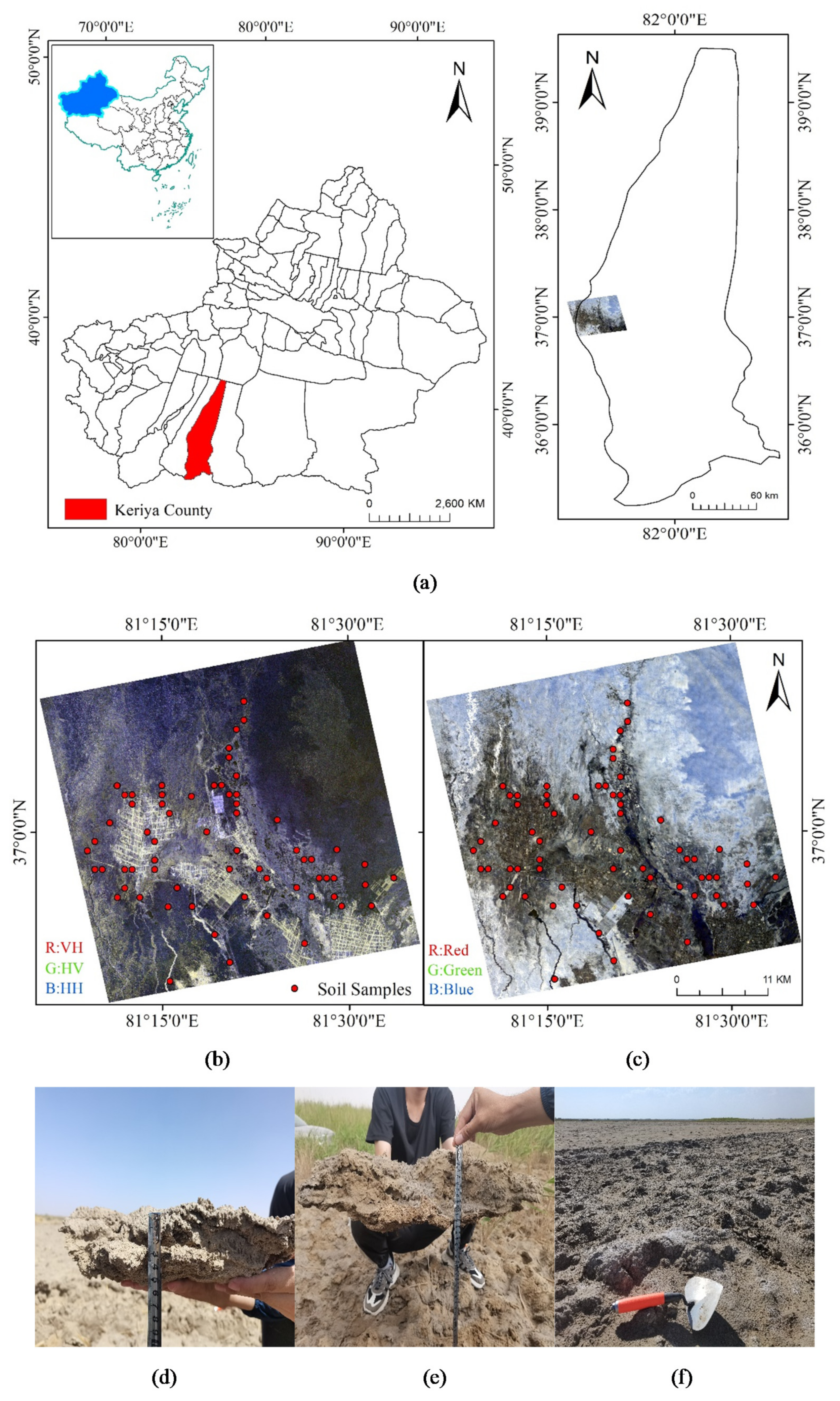
Figure 1.
Schematic diagram of the study area: (a) Location of the study area. (b) PALSAR-2 image of the study area (Red: VH, Green: HV, Blue: HH). (c) Landsat 8 image of the study area (Red: Red, Green: Green, Blue: Blue). (d,e) Thicker salt crusts in the study area. (f) Strongly salinized soil.
3. Data and Methods
3.1. Data
Phased-Array L-Band Synthetic Aperture Radar (PALSAR) is an L-band synthetic aperture radar sensor on the Earth observation satellite Advanced Land Observing Satellite (ALOS) launched by Japan, which is mainly used for mapping, regional observation, and disaster monitoring [45,46]. The full polarization (HH, HV, VH, VV) data on 23 April 2015, were acquired in this study. Because PALSAR is an active microwave sensor, it can observe features all day and all night, and the full polarization imaging also makes the images have more features reflection, which can better express the soil salt distribution and accumulation in the study area. The ALOS-PALSAR-2 data used in this paper are Level 1 images, which can be pre-processed in the SARscape5.2.1® modules of ENVI5.3®, including multi looking processing, 3 × 3 window refined Lee filtering, geocoding, and radiometric calibration, to obtain the standard quad polarization backward scattering coefficient map.
Landsat 8 is a satellite jointly developed and manufactured by NASA and USGS for medium resolution observations of the globe. The Landsat 8-OLI (OLI) has nine bands for effective monitoring of soil salinization [47,48]. To reduce the variability due to time, the Landsat 8-OLI satellite image of 26 April 2015 was selected in this paper. The images were pre-processed into different index operations. To roughly coincide with the imaging time, the field-sampled soils collected from 20 April to 1 May 2015 were selected for this study, and 65 representative sample points were selected to collect surface soil from 0 to 20 cm based on the regional extent, soil characteristics, vegetation distribution status, geomorphological features, and climatic conditions. The coordinates of each soil sample point were recorded by GPS and brought to the laboratory after oven drying, grinding, and filtering through a 1 mm sieve [49,50]. The drying method (105 °C incubator, 48 h) was used to determine the soil water content. After configuring a soil solution with a soil-to-water ratio of 1:5, the soil conductivity was determined by a conductivity meter at room temperature (25 °C). Finally, the total soluble salt content (in g/Kg) was calculated by establishing an equation between conductivity and total soluble salt [51].
3.2. Methods
3.2.1. Water Could Model
The study area is in an inland arid region, but the surface in the oasis region is still covered by a great deal of vegetation, whose scattering and absorption effects on microwave signals cannot be ignored, and to accurately obtain the backscattering coefficient of the sub-bedding soil, the interference of the vegetation layer on the scattering needs to be removed [52]. Attma et al. proposed the Water Could Model (WCM), which simplifies the scattering process of the microwave remote sensing by assuming that the vegetation layer is a horizontally homogeneous cloud layer and disregarding the scattering effect between the vegetation layer and the sub-bedding soil layer [53], with the following expressions:
where is the total backscatter coefficient; is the vegetation layer’s backscatter coefficient; is the soil surface’s backscatter coefficient; is the attenuation factor of penetrating the vegetation layer; is the vegetation water content; is the radar wave incidence angle; and , are the parameters of the vegetation. Table 1 shows the empirical parameters obtained from previous studies [54].

Table 1.
Empirical parameters of the WCM.
Bringing all parameters into the equation yields the bare soil backward scattering coefficient (Equation (4)).
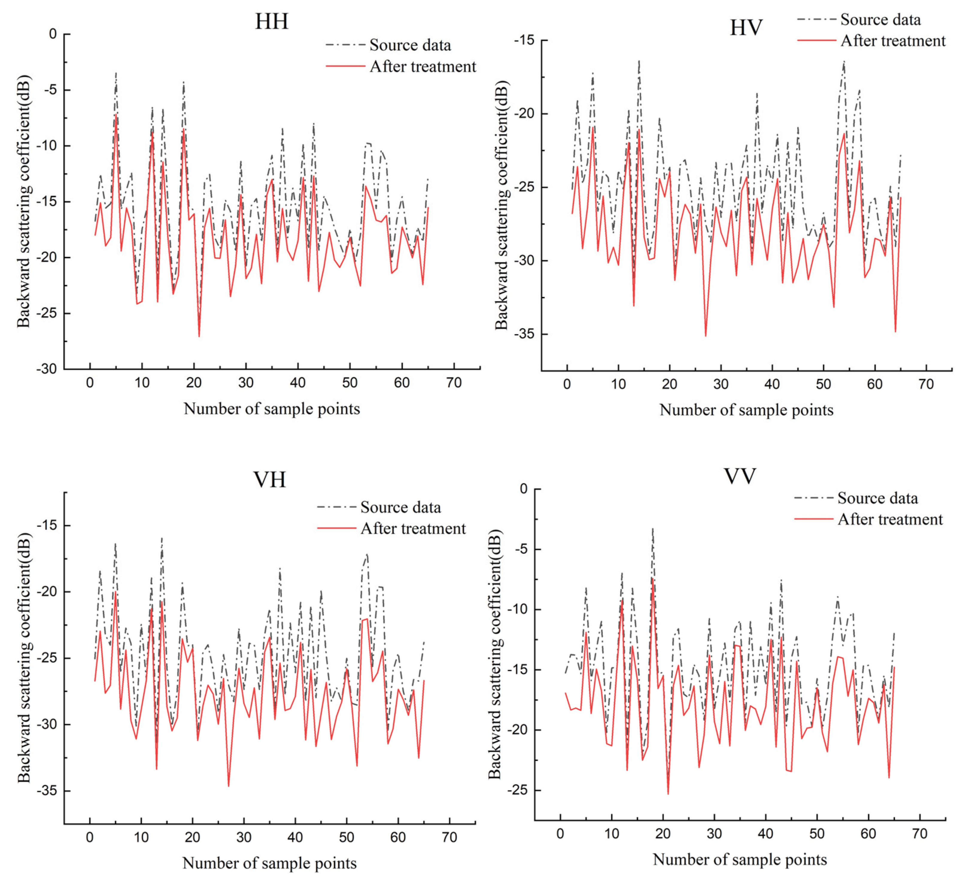
The results of the backscattering coefficients obtained after the WCM processing are shown in Figure 2.
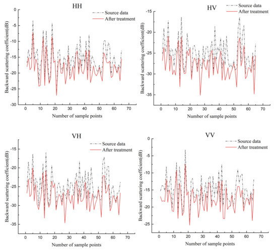
Figure 2.
Comparison of the WCM before and after processing.
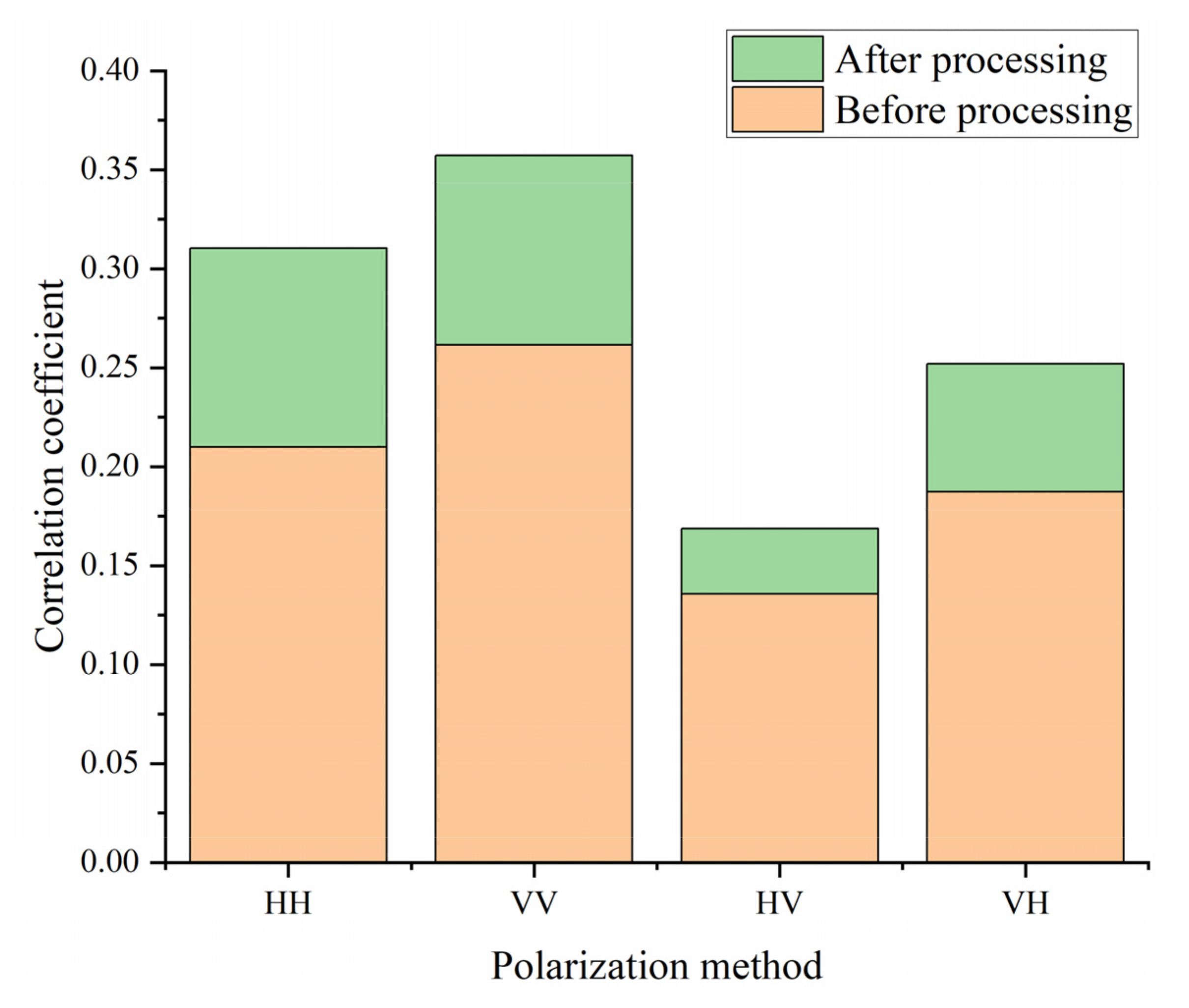
It can be seen from the figure that the backscattering coefficients of the four polarization methods are reduced after the treatment of the WCM. Figure 3 represents the correlation coefficients of the backscattering coefficients and soil salinity before and after the processing of the WCM, from which it can be seen that the correlation between the backscattering coefficients and soil salinity of all four polarization methods has improved after the treatment. It can be seen that the WCM can remove the interference of the vegetation layer on the backscattering coefficients in the study area.

Figure 3.
The correlation coefficients of the backscattering coefficients and soil salinity before and after the processing of the WCM.
3.2.2. Back-Propagation Neural Network (BPNN)
BPNN is a classical machine learning method whose algorithm was proposed by Rumelhart et al. in 1986 [55], and its operation is realized by two processes: forward propagation when the data flow is passed from the input layer to the implicit layer and then to the output layer, and if the desired output is not obtained in the output layer, the back propagation of the error signal is started, and the weights and thresholds are adjusted by feeding the errors back to the individual neurons. Forward and backward propagation is alternated to achieve the minimum value of the network error function [56,57]. The back propagation of the error signal makes the BPNN have a strong nonlinear fitting capability and is suitable for application to geography-related problems.
3.2.3. Support Vector Machine
Support vector machine is a machine learning algorithm developed on the theoretical basis of statistics and structural risk minimization [58]. It seeks the optimal plane for solving the original low-dimensional problem by transforming it into a high-dimensional space through kernel functions. Additionally, the goal of SVM is to obtain the optimal solution under the available information rather than the optimal solution under the number of samples and thus is suitable for problems with small samples [59,60]. By changing its kernel function and related parameters, SVM can be divided into two categories, support vector classification (SVC) and support vector regression (SVR), and the radial basis function is chosen as the kernel function of SVR in this paper. Radial basis functions are widely used for different dimensional and sample problems with their powerful nonlinear mapping ability [60]. However, the accuracy of the model simulation is largely affected by the penalty parameter C and the kernel parameters, so it needs to be optimized. The radial basis function is formulated as follows.
where x is the vector of the prediction factor; is the sample vector of the SVM; and is a kernel parameter.
3.2.4. Particle Swarm Optimization
Because of the complex nonlinear relationship between the selected inversion parameters and soil salinity in this article, particle swarm optimization (PSO) was used for the optimization of key parameters in the SVR model and BPNN model. The idea of the particle swarm algorithm is derived from the foraging behavior of birds and was first proposed by Kennedy and Eberhart [61]. The algorithm treats each solution of the optimization problem as a random particle, and by simulating the foraging process of birds, each particle has its random position and flight speed. During the iterative process, each particle records and updates its current position and velocity and records its optimal position and the optimal position of the population [62,63]. For example, in an optimal problem sought in an n-dimensional space, there are m particles forming a population, the position of the ith particle is denoted as xi = (xi1, xi2, xin) and the velocity is denoted as vi = (vi1, vi2, vin). The iterative formulas for updating the velocity and position of each particle in the population are as follows [64].
where i = 1, 2, 3, …, m; is the individual extreme point position; is the overall situation extreme point position; is the initial weight value of inertia, generally ranging from 0 to 1.4; , are the accelerating coefficients; and , are random numbers between 0 and 1.
The addition of the particle swarm algorithm allows the BPNN model to overcome the drawbacks of slow convergence and easy to fall into local optimal solutions, and the optimal weights and thresholds are proposed to determine the minimum grid error [57]. For the SVM model based on the principle of structural risk minimization, the addition of the PSO algorithm with global convergence could better ensure the rationality of the parameter optimization [64]. Therefore, the PSO algorithm is chosen to optimize the model in this paper.
4. Modelling Strategy
4.1. Model Variables
In this paper, through a large number of experiments, 18 polarization combinations with high correlation with the soil salinity in this study area were selected by the Pearson correlation coefficient method, and then the four with the highest correlation were selected: VV/VH (−0.4), VV − VH/VV + VH (0.41), HV − HH/HV + HH (0.46), and (HV2 − HH2)/(HV2 + HH2) (0.44) as model parameters to invert the soil salinity (e.g., Figure 4). In contrast to the spectral information-rich Landsat data, researchers have established numerous soil indices and vegetation indices for scientific studies. In this paper, the soil salinity index (SI-T) [65], salinity index (SI2) [66], salinity ratio index (SAIO) [33], and canopy response salinity index (CRSI) [16], which have a high correlation with soil salinity in the study area, were selected as model parameters based on previous studies. To make the predictions more accurate, this paper also included evapotranspiration, groundwater burial depth, and digital elevation data, which have been previously shown to be related to soil salinity [67,68,69], as shown in Table 2.
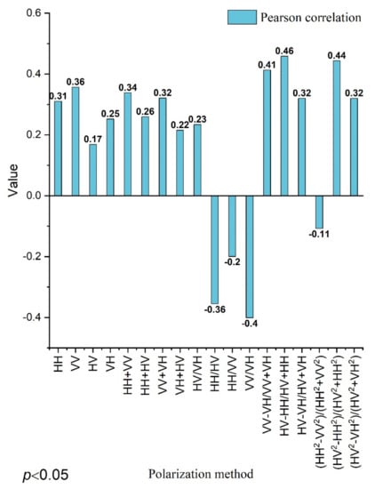
Figure 4.
Histogram of the polarization combination correlation coefficient. Both the polarization combination mode and the soil salinity in the study area are significantly correlated at the p < 0.05 level in the figure.
Table 2.
Table of model parameters.
When constructing the model, due to the different data sources, three sets of BPNN structures were constructed in this paper, whose input, the implicit and output layer neurons, were the PALSAR-2 data source: 7:75:1; Landsat 8 data source: 7:80:1; and PALSAR + Landsat data source: 11:155:1. The output layer of all three neural network models is soil salinity, and gradient descent algorithm with variable learning rate is used as the training function, with a learning rate of 0.01, 1000 iterations, and an allowable error of 0.0001. The structure of the PSO models for the three different data sources is the PALSAR-2 data source: 60 evolution times, a population size of 30; Landsat 8 data source: 60 evolution times; the inertia variable is 1 in all three models, and the accelerating coefficients are 2 and 1, respectively.
In this paper, the BPNN, SVR, PSO-BPNN, and PSO-SVR models were established in MATLAB®, and the model accuracy was evaluated by the Coefficient of Determination (R2) and Root Mean Square Error (RMSE) to evaluate the merits.
4.2. Data Division
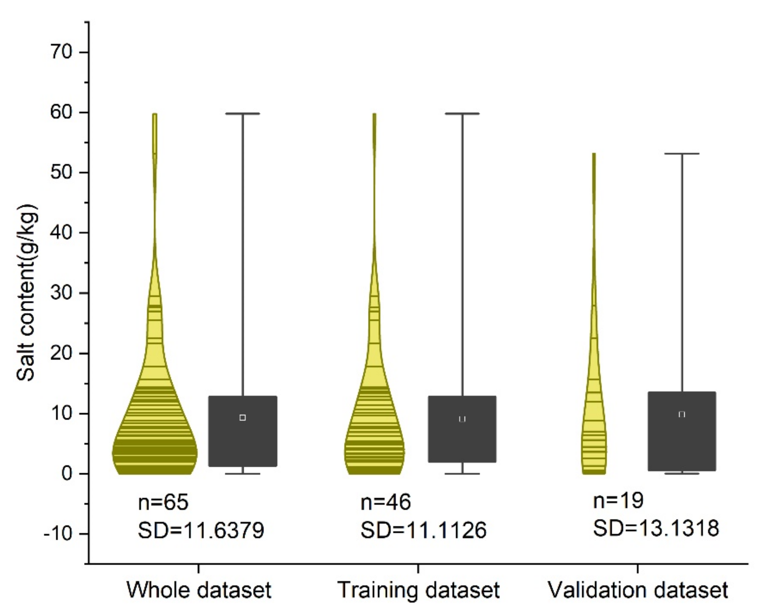
In this study, a total of 65 soil sample points were collected, with soil salinity ranging from 0.0046 to 59.7895 g/kg, and the mean value was 9.2930 g/kg with a standard deviation of 11.6379 g/kg. By referring to Wei et al.’s study, the conditional Latin Hypercube Sampling design (cLHS) was used to divide all sample points into training and validation sets in the ratio of 7:3 [70]. The training set has 46 soil sample points with salinity ranging from 0.0046 to 59.7895 g/kg, with a mean value of 8.7631 g/kg and a standard deviation of 11.1126 g/kg; the validation set has 19 soil sample points with salinity ranging from 0.0495 to 53.1814 g/kg, with a mean value of 10.5757 g/kg and a standard deviation of 13.1318 g/kg. As shown in Figure 5, the data characteristics of the three data sets were relatively similar.

Figure 5.
Sample distribution.
5. Results
To compare the predictive ability of the different models for soil salinity in the study area, different inversion parameters were brought into the models in this study, and the R2 and RMSE of the training and validation sets are shown in Table 3.
Table 3.
Accuracy table of simulation results.
As seen from Table 3, relative to the three data sets, the predicted values of the PSO-SVR model improved by 0.07 (PALSAR-2 data), 0.20 (Landsat 8-OLI data), and 0.19 (PALSAR + Landsat data) compared to the R2 of the SVR model, and the R2 of the PSO-BPNN model improved by 0.03 (PALSAR-2 data), 0.24 (Landsat 8-OLI data), and 0.12 (PALSAR + Landsat data). After adding PSO, the current optimal position of each particle is recorded when the model iterates, and based on the position of the individual in the whole, the algorithm determines whether the historical optimal solution of the particle population needs to be updated and continues to iterate on top of the optimal solution; thus, the simulation accuracy of both the SVR and BPNN models is improved.
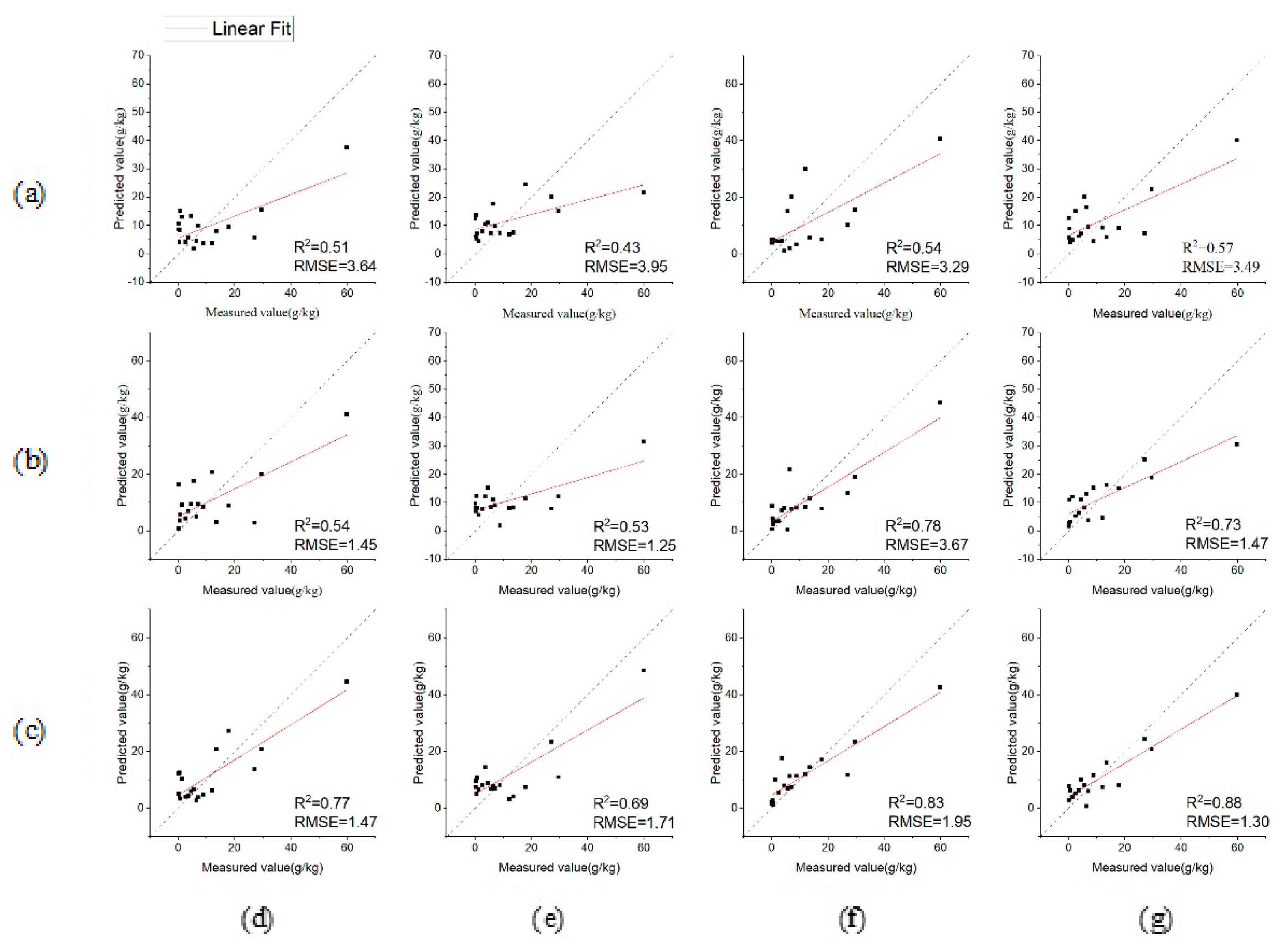
According to Table 2, the different input variables of the different data sources and different model input parameters affect the simulation accuracy of the model. However, the prediction accuracy of the three data sources in general is from high to low for PALSAR + Landsat, Landsat 8-OLI, and PALSAR-2. The scatter plots of the results predicted by the different data sources and different models are presented in Figure 6. From the figure, we can find that the predicted values of all models are low when the soil salinity is higher than 20 g/kg. The predicted values of the PALSAR + Landsat data source are less discrete compared with the single data source, indicating that the combination of multiple remote sensing data sources can reflect the soil salinity information in the study area more effectively; the predicted values of the model with PSO are relatively less discrete compared with the initial model. When Palsar2+Landsat is used as the data source, the simulated values of the PSO-SVR model are more uniformly distributed around the 1:1 line in the range of 0–20 g/kg, and the predicted values above 20 g/kg were lower than the predicted values but closer to the 1:1 line compared with other models, indicating that the model is relatively stable and has better accuracy.
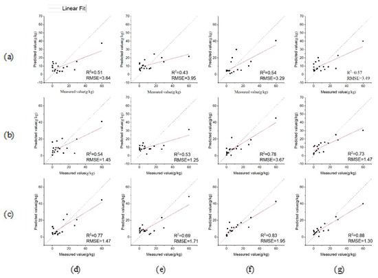
Figure 6.
R2 plots of the simulation results. Different rows represent different data sources: (a) PALSAR-2; (b) Landsat 8; (c) PALSAR + Landsat. Different columns represent different methods: (d) BPNN; (e) SVR; (f) PSO-BPNN; (g) PSO-SVR. The unit of RMSE is g/kg.
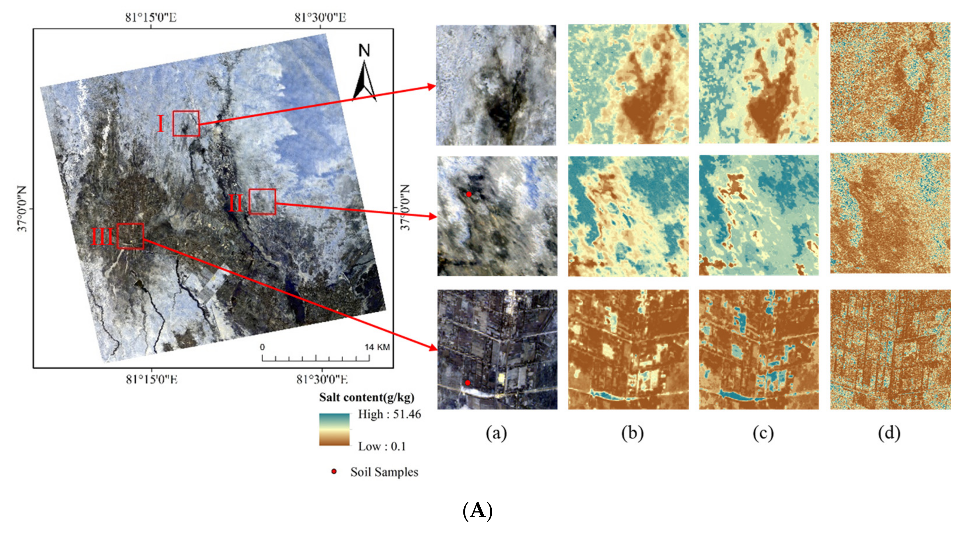
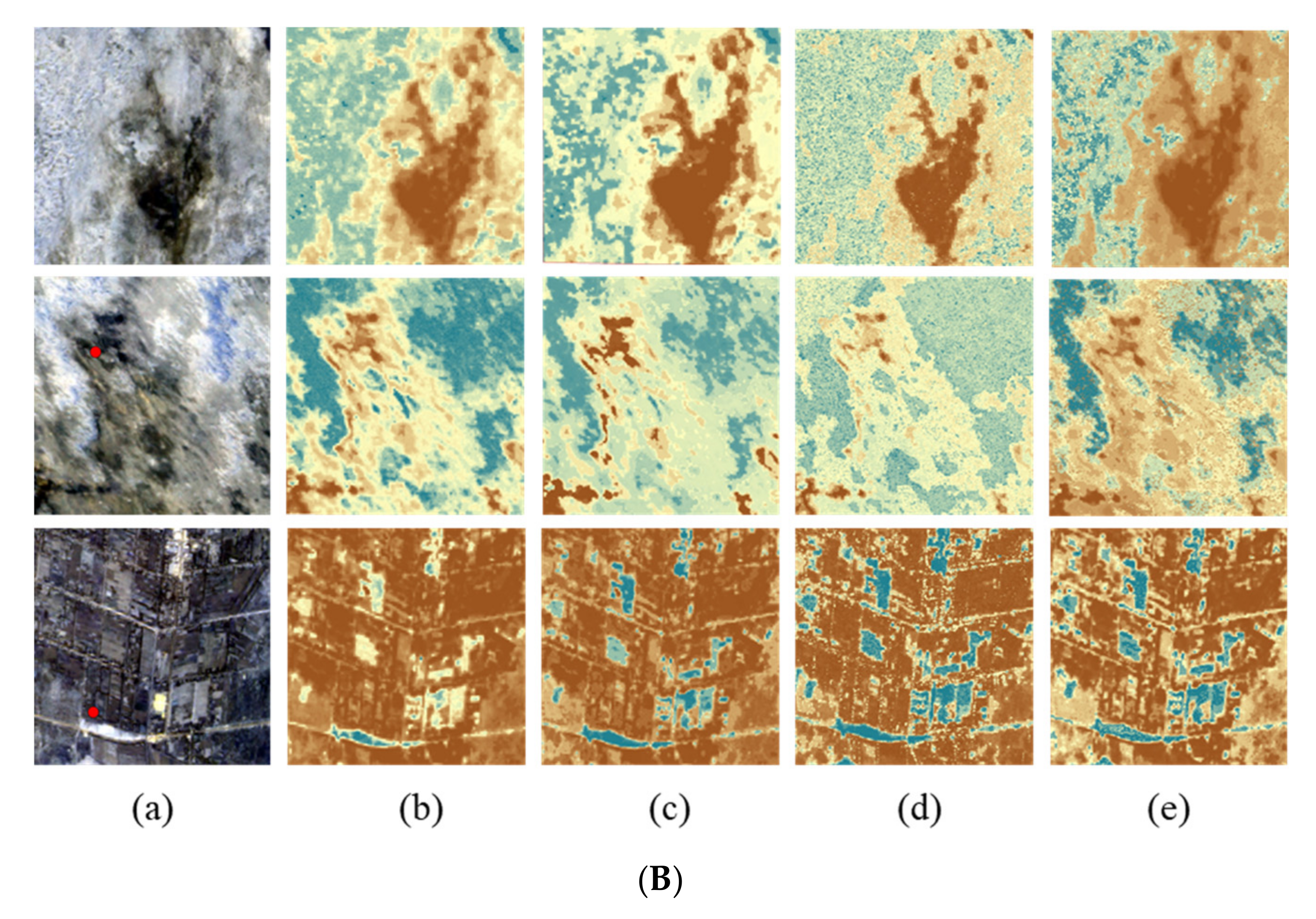
To compare the inversion results of the different data sources and different methods in a more detailed way. In this paper, three representative sub-study areas—I, II, and III—were selected to compare the local features of the inversion results. As shown in Figure 7A, sub-study areas I and II are at the edge of the oasis and are located at the intersection of the oasis and desert. Soil salinity is lower in oasis and higher in desert soils, resulting in more significant differences in soil salinity in the interlaced zone, which can better reflect the inversion results. Sub-study area III is in the interior of the oasis and can reflect the model inversion of soil salinity in the interior of the oasis. We found through our fieldwork that sub-study area I is located in an area of moderate salinity, sub-study area II is located in an area of more severe salinity, and sub area III is located within agricultural land with a low level of salinity, but with minor secondary salinity occurring. The inversion results of the model can also be better represented by different degrees of salinization. To compare the inversion results of different data sources, the PALSAR-2 data source, Landsat 8 data source, and PALSAR + Landsat data source were brought into the PSO-SVR model in this paper, and the inversion results are compared in the sub-study areas. As shown in Figure 7A, (a) indicates the Landsat 8 true color (RGB) images; (b) indicates the PALSAR + Landsat data source inversion results; (c) indicates the Landsat 8 data source inversion results, and (d) indicates the PALSAR-2 data source inversion results. In sub-study areas I and II, the inversion results from the Landsat 8 data source are closer to the soil salinity distribution characteristics of the sub-study area than the PALSAR-2 data source; the inversion results from the PALSAR-2 data source are too fragmented and invert areas with high salinity as low value areas, but retain the feature boundary characteristics well. In sub-study area III, the Landsat 8 data source has too-high inversion values for field soil salinity, and the PALSAR-2 data source inversion results are similarly too fragmented and do not quite match the soil salinity distribution characteristics of the sub-study areas. In the three sub-study areas, the inversion results of the PALSAR + Landsat data sources combine the high-resolution texture information of PALSAR-2 and the rich spectral information of Landsat 8 to make the inversion results more detailed and better reflect the variability in soil salinity. To compare the inversion results of the different models, PALSAR + Landsat data were brought into the PSO-SVR, PSO-BPNN, SVR, and BPNN models in this paper to compare the inversion results in the sub-study area. As shown in Figure 7B, (a) indicates Landsat 8 true color (RGB) image; (b) indicates the PSO-SVR model inversion results; (c) indicates the PSO-BPNN model inversion results; (d) indicates the SVR model inversion results, and (e) indicates the BPNN model inversion results. As can be seen from the figure, the inversion results of the model without PSO are relatively less good and do not reflect well the differences in soil salinity between the oasis and desert interlacing zones. The inversion values of soil salinity inside the oasis are higher and do not match the soil salinization in the sub-study areas. The inversion results of the PSO-SVR model are more detailed and well represent the differences in soil salinity in different areas, both in the interlaced zone and within the oasis, and are more consistent with the soil salinity distribution characteristics of the sub-study areas (sub-study area I moderate salinity, sub-study area II high salinity, and sub-study area III low salinity) than those of the PSO-BPNN model. With Table 3, the accuracy of the predicted values was improved by bringing the PALSAR + Landsat data source into the PSO-SVR model. Therefore, the PSO-SVR model and PALSAR + Landsat data source were finally selected in this paper to invert the soil salinity in the study area, and the results are shown in Figure 8. To avoid errors as much as possible, the river area in the study area is masked in this paper.


Figure 7.
(A) The PALSAR + Landsat data source, Landsat 8 data source, and PALSAR-2 data source were brought into the PSO-SVR model, respectively, and the inversion results of the three data sources are compared in the subregion. I, II, and III sub-study areas. (a) True-color Landsat 8 OLI images. (b) Inversion results of the PALSAR + Landsat data source. (c) Inversion results of the Landsat 8 data source. (d) Inversion results of the PALSAR-2 data source. (B). The PALSAR + Landsat data source were brought into the PSO-SVR, PSO-BPNN, SVR, and BPNN models, respectively, and the inversion results of the four models were compared in the same three sub-regions as above. (a) True-color Landsat 8-OLI image. (b) Inversion results of the PSO-SVR model. (c) Inversion results of the PSO-BPNN model. (d) Inversion results of the SVR model. (e) Inversion results of the BPNN model.
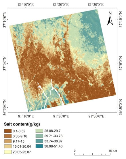
Figure 8.
The inversion results of soil salinity in the study area using the optimal model PSO-SVR and the optimal data source PALSAR + Landsat. The white part is the masked river area.
6. Discussion
6.1. Model Analysis
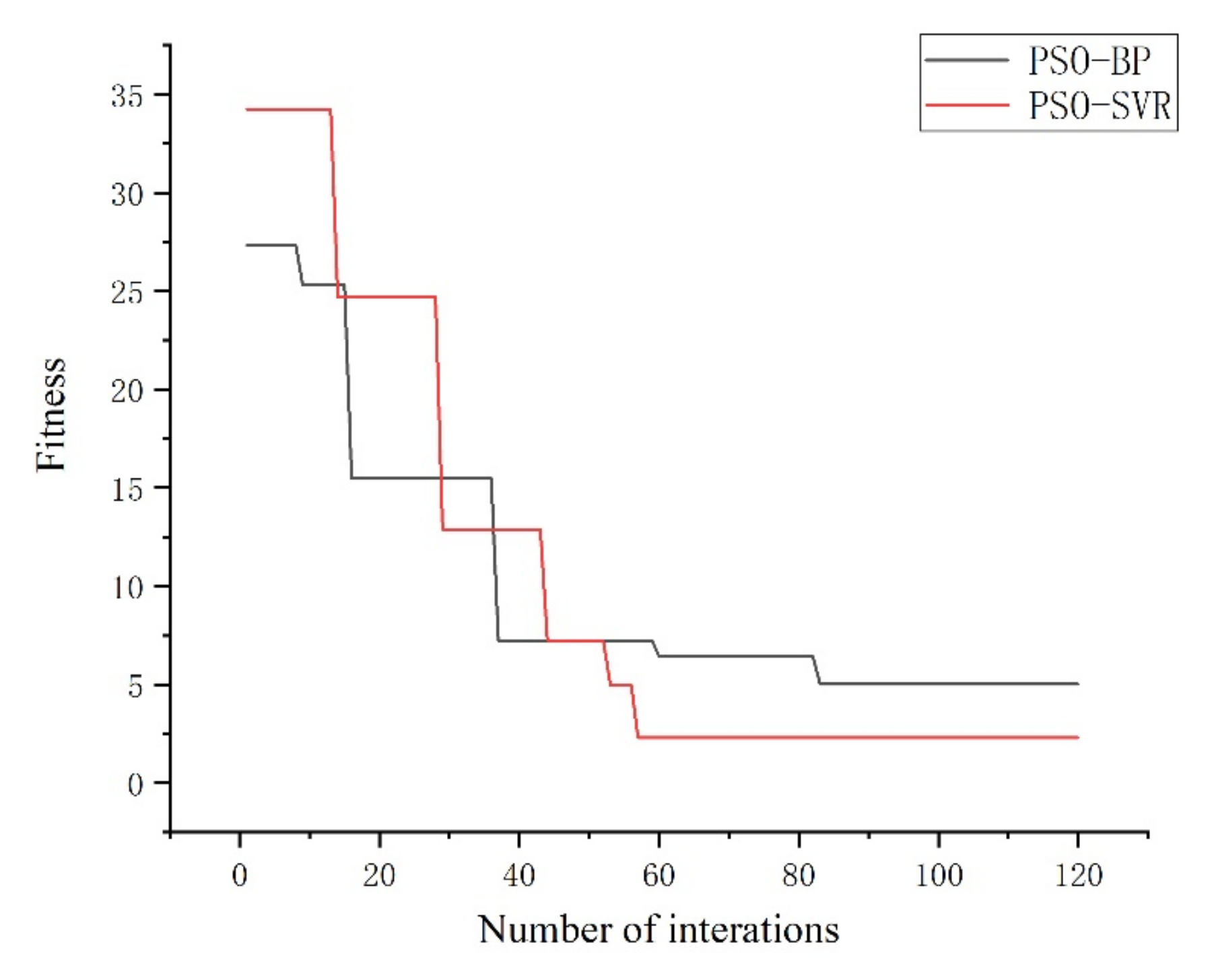
In this paper, four methods, namely, SVR, BPNN, PSO-SVR, and PSO-BPNN, were used to invert soil salinity. According to the results in Table 3 and Figure 6, it was found that the inversion accuracy of the SVR and BPNN models were relatively close before the addition of PSO, while the inversion results of the PSO-SVR model were better than the PSO-BPNN model after the addition of PSO, and the effect was improved when compared to the original model The reasons for this are as follows: (1) Compared with the BPNN model, the SVR model relies more on the kernel function and the selection of relevant parameters. With the addition of PSO, the SVR model can automatically iterate through the particles to optimize the key parameters within a given range, thus improving the overall accuracy of the model. As can be seen from Figure 9, the PSO-SVR model converges faster and more accurately than the PSO-BPNN model during training, Therefore, the PSO-SVR model is more applicable in this study area. (2) Compared with the BPNN, the SVR model is more suitable for small sample studies. The theoretical basis of nonlinear mapping allows the SVR model to determine the final results with fewer key samples and avoids the drawback of falling into a local optimum, similar to the BPNN model. Similar conclusions were presented in the study of soil salinity in Yanqi, Xinjiang, by Hong Jiang et al. [71].

Figure 9.
Adaptation curves.
6.2. Analysis of Model Variables
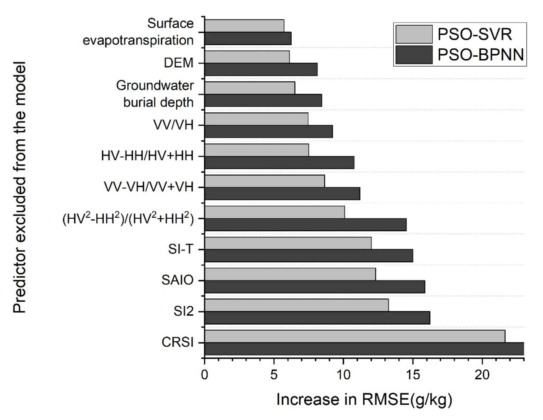
The SVR and BPNN models selected for this paper do not provide variable importance rankings, but refer to Kennedy Were et al.’s study in Eastern Mau Forest Reserve [59]. In this paper, the importance of the predictor variables is represented by removing them from the PSO-SVR and PSO-BPNN models in turn and looking at the degree of increase in RMSE of their prediction results. It can be seen from Figure 10 that the soil, vegetation index, and polarization combinations extracted from the remote sensing data sources have a greater influence on the model for both the PSO-SVR and PSO-BPNN models. The reason may be that in arid and semi-arid regions, vegetation and soil characteristics are indispensable environmental variables for the inversion of soil salinity [72]. However, in terms of remote sensing data sources, the four indices extracted from the Landsat 8 data source are more important to the model than the four polarization combinations extracted from the PALSAR-2 data source. This may be due to the low direct correlation of the bands (HH, HV, VH, VV) in the PALSAR-2 data source with the soil salinity in the study area (as shown in Figure 4), resulting in their combination being less important to the model than the Landsat 8 data source. Relative to all eleven variables, CRSI had the highest importance, indicating that it was the strongest indicator of soil salt salinity in the model of this paper. Probably due to the CRSI, which contains all visible bands and one near-infrared band, it highlights the small peak of vegetation reflectance at the 400–500 nm wavelengths and the sudden change in reflectance that occurs between the red and near-infrared bands [73]. Most of the sampling sites in this paper are in the interior of the oasis, so CRSI is more sensitive to soil salinity in this study area. Kristen Whitney et al. used CRSI as the primary basis for their soil salinity study in Farmland of California’s western San Joaquin Valley [74]. Wang et al. also proposed CRSI as one of the important indicators for soil salinity identification in their study of quantitative soil salinity assessment in three oases in Xinjiang, again validating the important role of CRSI for soil salinity studies [75]. This result is similar to the findings of previous studies. Although this study exemplifies the importance of the model input variables by the above methods, it is still a potential uncertainty in this study for the black box problem involved in machine learning. In future studies, we will attempt to solve this problem by other methods.
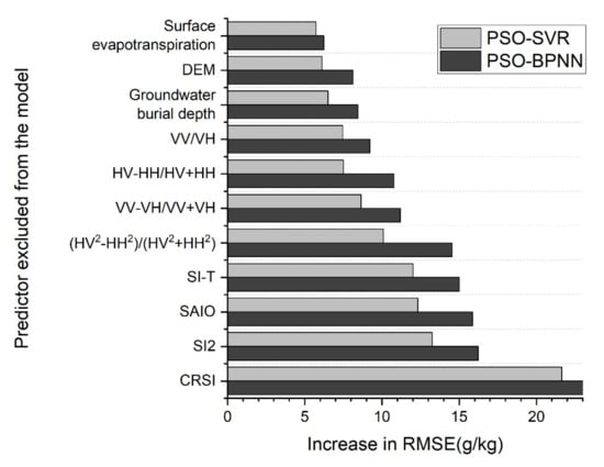
Figure 10.
Variable importance is shown by the increase in the RMSEs of the PSO-SVR and PSO-BPNN models after excluding a predictor.
6.3. Data Analysis
In this paper, different data sources were used to invert the soil salinity of the field oasis (see Table 2 and Figure 6). The inversion results were greatly influenced by different data sources, and the prediction effect of the PALSAR data source was not that of the Landsat data source when compared with a single data source. The results might be as follows: (1) The imaging mechanism of PALSAR data is different from that of optical data, resulting in its being seriously affected by speckle noise, and although its image resolution is higher, its spectral information is not as rich as that of Landsat data. (2) Soil salinity in arid areas is affected by many factors; the real and imaginary parts of the dielectric constant of the soil receive the effect of water and salt content, respectively. Although the soil salinity characteristics can be enhanced to some extent by band combination, the effect of water content on the dielectric constant still cannot be eliminated. In contrast, Landsat images can better show the soil salinity characteristic values through more mature spectral indices, thus improving the prediction accuracy of the model. (3) The influence of vegetation in the study area should not be neglected. Although this paper uses the WCM to remove the interference of vegetation to a certain extent, its effect is still different for the densely vegetated area and the less vegetated area in the oasis-desert interlacing zone, and it cannot completely eliminate the influence of vegetation, resulting in a large noise error in the PALSAR image. (4) It has been shown that surface roughness is also one of the important factors affecting the backscattering coefficient of features [76,77]. In this study area, the topography is complex, as there are many zones where the Gobi desert intersects with the vegetated areas; therefore, there is some difficulty in characterizing the surface roughness, which affects the correlation between the backscattering coefficient and the soil salinity. From the above analysis, it can be seen that it is still difficult to invert soil salinity using only a single radar data source [78,79], and in future research, multiple methods or multiple sources of data are needed to reduce the effect of noise.
6.4. Soil Salinity Distribution in the Study Area
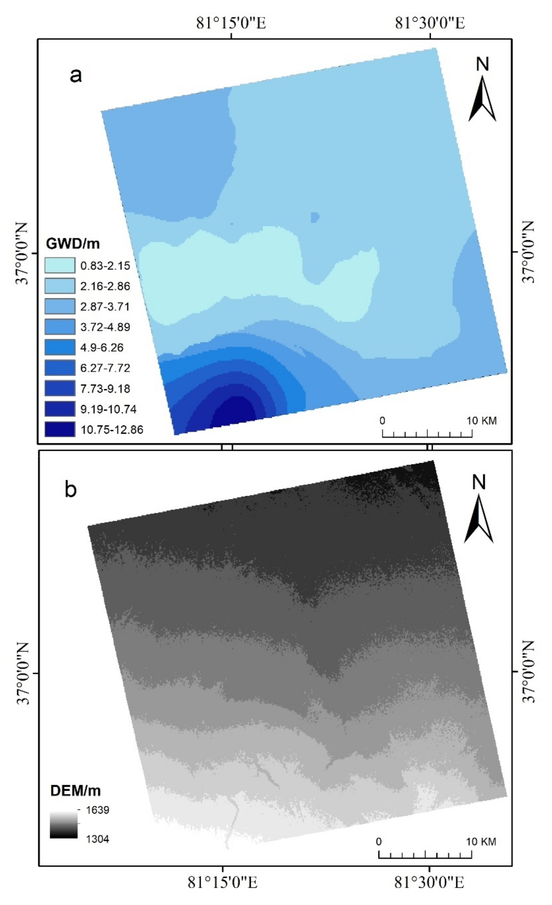
From the inversion results of this paper, the soil salinity in the study area shows a high north and south and low middle, which is similar to the results of previous studies [25]. Figure 11 shows the spatial interpolation map and DEM map of the groundwater level in this area, and by looking at the map, we can see that the northern part of the area has a low-lying topography and shallow groundwater levels. The reason for the higher salinity of the soil in the northern part of this area may be due to the shallow water table, the salts in the southern soil are brought to the surface due to capillary action, and the dry climate causes the water to evaporate, leaving the salts, and causing the salinization. Second, the terrain in the northern part of the area is relatively flat, groundwater moves mostly in a vertical manner, and horizontal runoff is effectively stagnant, which forms a good environment for soil salinity accumulation. In the southern part of the area, agricultural activities are more significant, and according to Figure 8 that the soil salinity is high around the cultivated land in the southern region, which may be due to unscientific cultivation practices that lead to secondary salinization.
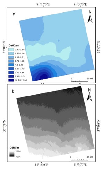
Figure 11.
Schematic diagram of (a) GWD and (b) DEM in the study area.
7. Conclusions
In this paper, we combine particle swarm algorithm and machine learning to propose a method to combine multi-source remote sensing data for soil salinity inversion, and the main findings are as follows: (1) By comparing the simulation results of different models, we found that the prediction accuracy of both the BPNN and SVR models was significantly improved by adding PSO, and the prediction values of the PSO-SVR model are improved by 0.07 compared to the R2 of the SVR model (PALSAR-2 data), 0.20 (Landsat 8-OLI data), and 0.19 (PALSAR + Landsat data). The PSO-BPNN model improved the R2 compared to the BPNN model by 0.03 (PALSAR-2 data), 0.24 (Landsat 8-OLI data), and 0.12 (PALSAR + Landsat data). This indicates that the addition of PSO can have improved model accuracy. The simulation results of the PSO-SVR model are better than those of PSO-BPNN, indicating that the former is more suitable for the study of soil salinization in small areas. The final comparison showed the PSO-SVR model to be the best model for inversion of soil salinity in this area. (2) Comparing the inversion result plots, we found that using only a single microwave image to invert the soil salinity is not as effective as using the Landsat image. The combination of PALSAR’s high-resolution texture information and Landsat’s rich spectral information can better reflect the distribution of soil salinity in the study area. (3) The soil salinity in the study area tends to be low in the middle and high at the edges, which may be due to the low-lying topography in the north of the study area and the shallow depth of the groundwater, making it vulnerable to salinization; in the south, there are more agricultural activities, and unscientific irrigation methods may lead to secondary salinization. The surface runoff formed by the high terrain in the south may wash salt into the study area territory, intensifying the occurrence of salinization.
Author Contributions
All authors contributed in a substantial way to the manuscript. Methodology, Q.W.; formal analysis, Q.W.; data curation, Q.W.; writing—original draft preparation, Q.W.; writing—review and editing, Q.W.; conceptualization, I.N.; investigation, I.N.; project administration, I.N.; funding acquisition, M.G.; visualization, B.X. All authors have read and agreed to the published version of the manuscript.
Funding
This research was funded by the National Natural Science Foundation of China [No. 42061065 and No. U1703237].
Institutional Review Board Statement
Not applicable.
Informed Consent Statement
Not applicable.
Data Availability Statement
Not applicable.
Acknowledgments
We extend our hearty gratitude to the anonymous reviewers of this manuscript for their constructive comments and helpful suggestions provided during the preparation.
Conflicts of Interest
The authors declare no conflict of interest.
References
- Li, P.; Qian, H.; Wu, J. Conjunctive use of groundwater and surface water to reduce soil salinization in the Yinchuan Plain, North-West China. Int. J. Water Resour. Develop. 2018, 34, 337–353. [Google Scholar] [CrossRef]
- Wang, F.; Shi, Z.; Biswas, A.; Yang, S.; Ding, J. Multi-algorithm comparison for predicting soil salinity. Geoderma 2020, 365, 114211. [Google Scholar] [CrossRef]
- Rozema, J.; Flowers, T. Crops for a salinized world. Science 2008, 322, 1478–1480. [Google Scholar] [CrossRef]
- Singh, A. Soil salinization and waterlogging: A threat to environment and agricultural sustainability. Ecol. Indic. 2015, 57, 128–130. [Google Scholar] [CrossRef]
- Nunez, M.; Finkbeiner, M. A Regionalised Life Cycle Assessment Model to Globally Assess the Environmental Implications of Soil Salinization in Irrigated Agriculture. Environ. Sci. Technol. 2020, 54, 3082–3090. [Google Scholar] [CrossRef] [PubMed] [Green Version]
- Chang, X.; Gao, Z.; Wang, S.; Chen, H. Modelling long-term soil salinity dynamics using SaltMod in Hetao Irrigation District, China. Comp. Electron. Agric. 2019, 156, 447–458. [Google Scholar] [CrossRef]
- Yang, H.; Chen, Y.; Zhang, F. Evaluation of comprehensive improvement for mild and moderate soil salinization in arid zone. PLoS ONE 2019, 14, e0224790. [Google Scholar] [CrossRef]
- Jiang, Q.; Peng, J.; Biswas, A.; Hu, J.; Zhao, R.; He, K.; Shi, Z. Characterising dryland salinity in three dimensions. Sci. Total Environ. 2019, 682, 190–199. [Google Scholar] [CrossRef] [PubMed]
- Szoboszlay, M.; Nather, A.; Liu, B.; Carrillo, A.; Castellanos, T.; Smalla, K.; Jia, Z.; Tebbe, C.C. Contrasting microbial community responses to salinization and straw amendment in a semiarid bare soil and its wheat rhizosphere. Sci. Rep. 2019, 9, 9795. [Google Scholar] [CrossRef]
- Xu, Z.; Shao, T.; Lv, Z.; Yue, Y.; Liu, A.; Long, X.; Zhou, Z.; Gao, X.; Rengel, Z. The mechanisms of improving coastal saline soils by planting rice. Sci. Total Environ. 2020, 703, 135529. [Google Scholar] [CrossRef] [PubMed]
- Amezketa, E. An integrated methodology for assessing soil salinization, a pre-condition for land desertification. J. Arid Environ. 2006, 67, 594–606. [Google Scholar] [CrossRef]
- Singh, A. Soil salinization management for sustainable development: A review. J. Environ. Manag. 2021, 277, 111383. [Google Scholar] [CrossRef]
- Jiang, S.Q.; Yu, Y.N.; Gao, R.W.; Wang, H.; Zhang, J.; Li, R.; Long, X.H.; Shen, Q.R.; Chen, W.; Cai, F. High-throughput absolute quantification sequencing reveals the effect of different fertilizer applications on bacterial community in a tomato cultivated coastal saline soil. Sci. Total Environ. 2019, 687, 601–609. [Google Scholar] [CrossRef] [PubMed]
- Li-ping, L.; Xiao-hua, L.; Hong-bo, S.; Zhao-Pu, L.; Ya, T.; Quan-suo, Z.; Jun-qin, Z. Ameliorants improve saline–alkaline soils on a large scale in northern Jiangsu Province, China. Ecol. Eng. 2015, 81, 328–334. [Google Scholar] [CrossRef]
- Yang, H.; Chen, Y.; Zhang, F.; Xu, T.; Cai, X. Prediction of salt transport in different soil textures under drip irrigation in an arid zone using the SWAGMAN Destiny model. Soil Res. 2016, 54, 869–879. [Google Scholar] [CrossRef]
- Metternicht, G.I.; Zinck, J.A. Remote sensing of soil salinity: Potentials and constraints. Remote Sens. Environ. 2003, 85, 1–20. [Google Scholar] [CrossRef]
- Peng, J.; Biswas, A.; Jiang, Q.; Zhao, R.; Hu, J.; Hu, B.; Shi, Z. Estimating soil salinity from remote sensing and terrain data in southern Xinjiang Province, China. Geoderma 2019, 337, 1309–1319. [Google Scholar] [CrossRef]
- Ivushkin, K.; Bartholomeus, H.; Bregt, A.K.; Pulatov, A.; Kempen, B.; de Sousa, L. Global mapping of soil salinity change. Remote Sens. Environ. 2019, 231, 111260. [Google Scholar] [CrossRef]
- El Harti, A.; Lhissou, R.; Chokmani, K.; Ouzemou, J.-e.; Hassouna, M.; Bachaoui, E.M.; El Ghmari, A. Spatiotemporal monitoring of soil salinization in irrigated Tadla Plain (Morocco) using satellite spectral indices. Int. J. Appl. Earth Obs. Geoinf. 2016, 50, 64–73. [Google Scholar] [CrossRef]
- Jiang, H.; Shu, H.; Lei, L.; Xu, J. Estimating soil salt components and salinity using hyperspectral remote sensing data in an arid area of China. J. Appl. Remote Sens. 2017, 11, 016043. [Google Scholar] [CrossRef] [Green Version]
- Khadim, F.K.; Su, H.; Xu, L.; Tian, J. Soil salinity mapping in Everglades National Park using remote sensing techniques and vegetation salt tolerance. Phys. Chem. Earth Parts A/B/C 2019, 110, 31–50. [Google Scholar] [CrossRef]
- Wang, Z.; Zhang, F.; Zhang, X.; Chan, N.W.; Kung, H.-t.; Zhou, X.; Wang, Y. Quantitative Evaluation of Spatial and Temporal Variation of Soil Salinization Risk Using GIS-Based Geostatistical Method. Remote Sens. 2020, 12, 2405. [Google Scholar] [CrossRef]
- Saha, S. Microwave remote sensing in soil quality assessment. Int. Arch. Photogramm. Remote Sens. Spat. Inf. Sci. 2011, 38, W20. [Google Scholar] [CrossRef] [Green Version]
- Romanov, A.; Khvostov, I.; Sukovatova, A.Y. Seasonal variations of microwave radiation of saline soils in the Kulunda steppe on evidence derived from SMOS. In Proceedings of the 2017 Progress In Electromagnetics Research Symposium-Spring (PIERS), St. Petersburg, Russia, 22–25 May 2017; pp. 3025–3031. [Google Scholar]
- Nurmemet, I.; Sagan, V.; Ding, J.-L.; Halik, Ü.; Abliz, A.; Yakup, Z. A WFS-SVM Model for Soil Salinity Mapping in Keriya Oasis, Northwestern China Using Polarimetric Decomposition and Fully PolSAR Data. Remote Sens. 2018, 10, 598. [Google Scholar] [CrossRef] [Green Version]
- Wu, W.; Zucca, C.; Muhaimeed, A.S.; Al-Shafie, W.M.; Fadhil Al-Quraishi, A.M.; Nangia, V.; Zhu, M.; Liu, G. Soil salinity prediction and mapping by machine learning regression in Central Mesopotamia, Iraq. Land Degrad. Develop. 2018, 29, 4005–4014. [Google Scholar] [CrossRef]
- Li, Y.-Y.; Zhao, K.; Ding, Y.-L.; Ren, J.-H.; Li, Y. An empirical method for soil salinity and moisture inversion in west of Jilin. In Proceedings of the 2013 the International Conference on Remote Sensing, Environment and Transportation Engineering (RSETE 2013), Nanjing, China, 26–28 July 2013; p. 1921. [Google Scholar]
- Gong, H.; Shao, Y.; Brisco, B.; Hu, Q.; Tian, W. Modeling the dielectric behavior of saline soil at microwave frequencies. Can. J. Remote Sens. 2013, 39, 17–26. [Google Scholar] [CrossRef] [Green Version]
- Periasamy, S.; Shanmugam, R.S. Multispectral and Microwave Remote Sensing Models to Survey Soil Moisture and Salinity. Land Degrad. Develop. 2017, 28, 1412–1425. [Google Scholar] [CrossRef]
- Taghadosi, M.M.; Hasanlou, M.; Eftekhari, K. Soil salinity mapping using dual-polarized SAR Sentinel-1 imagery. Int. J. Remote Sens. 2018, 40, 237–252. [Google Scholar] [CrossRef]
- Romanov, A.N.; Khvostov, I.V. On the Validation of Satellite Microwave Remote Sensing Data under Soil Salinity Conditions. Izv. Atmos. Ocean. Phys. 2020, 55, 1033–1040. [Google Scholar] [CrossRef]
- Dong, L.; Wang, W.; Xu, F.; Wu, Y. An Improved Model for Estimating the Dielectric Constant of Saline Soil in C-Band. IEEE GeoSci. Remote Sens. Lett. 2021, 19, 1–5. [Google Scholar] [CrossRef]
- Scudiero, E.; Skaggs, T.H.; Corwin, D.L. Regional-scale soil salinity assessment using Landsat ETM + canopy reflectance. Remote Sens. Environ. 2015, 169, 335–343. [Google Scholar] [CrossRef] [Green Version]
- Asfaw, E.; Suryabhagavan, K.V.; Argaw, M. Soil salinity modeling and mapping using remote sensing and GIS: The case of Wonji sugar cane irrigation farm, Ethiopia. J. Saudi Soc. Agric. Sci. 2018, 17, 250–258. [Google Scholar] [CrossRef] [Green Version]
- Habibi, V.; Ahmadi, H.; Jafari, M.; Moeini, A. Quantitative assessment of soil salinity using remote sensing data based on the artificial neural network, case study: Sharif Abad Plain, Central Iran. Model. Earth Syst. Environ. 2020, 7, 1373–1383. [Google Scholar] [CrossRef]
- Pan, X.; Chen, Y.; Cui, J.; Peng, Z.; Fu, X.; Wang, Y.; Men, M. Accuracy analysis of remote sensing index enhancement for SVM salt inversion model. Geocarto Int. 2021, 1–18. [Google Scholar] [CrossRef]
- Mashimbye, Z.E.; Cho, M.A.; Nell, J.P.; De Clercq, W.P.; Van Niekerk, A.; Turner, D.P. Model-Based Integrated Methods for Quantitative Estimation of Soil Salinity from Hyperspectral Remote Sensing Data: A Case Study of Selected South African Soils. Pedosphere 2012, 22, 640–649. [Google Scholar] [CrossRef]
- Zhang, J.; Zhang, Z.; Chen, J.; Chen, H.; Jin, J.; Han, J.; Wang, X.; Song, Z.; Wei, G. Estimating soil salinity with different fractional vegetation cover using remote sensing. Land Degrad. Develop. 2020, 32, 597–612. [Google Scholar] [CrossRef]
- Ding, J.; Yu, D. Monitoring and evaluating spatial variability of soil salinity in dry and wet seasons in the Werigan–Kuqa Oasis, China, using remote sensing and electromagnetic induction instruments. Geoderma 2014, 235–236, 316–322. [Google Scholar] [CrossRef]
- Allbed, A.; Kumar, L.; Sinha, P. Mapping and Modelling Spatial Variation in Soil Salinity in the Al Hassa Oasis Based on Remote Sensing Indicators and Regression Techniques. Remote Sens. 2014, 6, 1137–1157. [Google Scholar] [CrossRef] [Green Version]
- Aldabaa, A.A.A.; Weindorf, D.C.; Chakraborty, S.; Sharma, A.; Li, B. Combination of proximal and remote sensing methods for rapid soil salinity quantification. Geoderma 2015, 239–240, 34–46. [Google Scholar] [CrossRef] [Green Version]
- Zhang, X.; Huang, B. Prediction of soil salinity with soil-reflected spectra: A comparison of two regression methods. Sci. Rep. 2019, 9, 5067. [Google Scholar] [CrossRef]
- Yang, X. The oases along the Keriya River in the Taklamakan Desert, China, and their evolution since the end of the last glaciation. Environ. Geol. 2001, 41, 314–320. [Google Scholar] [CrossRef]
- Seydehmet, J.; Lv, G.; Nurmemet, I.; Aishan, T.; Abliz, A.; Sawut, M.; Abliz, A.; Eziz, M. Model Prediction of Secondary Soil Salinization in the Keriya Oasis, Northwest China. Sustainability 2018, 10, 656. [Google Scholar] [CrossRef] [Green Version]
- Meynart, R.; Suzuki, S.; Neeck, S.P.; Kankaku, Y.; Osawa, Y.; Shimoda, H. Development status of PALSAR-2 onboard ALOS-2. In Proceedings of the Sensors, Systems, and Next-Generation Satellites XV, Prague, Czech Republic, 19–22 September 2011. [Google Scholar]
- Arikawa, Y.; Saruwatari, H.; Hatooka, Y.; Suzuki, S. ALOS-2 launch and early orbit operation result. In Proceedings of the 2014 IEEE geoscience and remote sensing symposium, Quebec City, QC, Canada, 13–18 July 2014; pp. 3406–3409. [Google Scholar]
- Roy, D.P.; Wulder, M.A.; Loveland, T.R.; Woodcock, C.E.; Allen, R.G.; Anderson, M.C.; Helder, D.; Irons, J.R.; Johnson, D.M.; Kennedy, R.; et al. Landsat-8: Science and product vision for terrestrial global change research. Remote Sens. Environ. 2014, 145, 154–172. [Google Scholar] [CrossRef] [Green Version]
- Vermote, E.; Justice, C.; Claverie, M.; Franch, B. Preliminary analysis of the performance of the Landsat 8/OLI land surface reflectance product. Remote Sens. Environ. 2016, 185, 46–56. [Google Scholar] [CrossRef]
- Wang, S.; Chen, Y.; Wang, M.; Zhao, Y.; Li, J. SPA-Based Methods for the Quantitative Estimation of the Soil Salt Content in Saline-Alkali Land from Field Spectroscopy Data: A Case Study from the Yellow River Irrigation Regions. Remote Sens. 2019, 11, 967. [Google Scholar] [CrossRef] [Green Version]
- Bao, S. Soil Agrochemical Analysis; China Agricultural Press: Beijing, China, 2000; pp. 180–181. [Google Scholar]
- Abuelgasim, A.; Ammad, R. Mapping soil salinity in arid and semi-arid regions using Landsat 8 OLI satellite data. Remote Sens. Appl. Soc. Environ. 2019, 13, 415–425. [Google Scholar] [CrossRef]
- Zhang, L.; Lv, X.; Chen, Q.; Sun, G.; Yao, J. Estimation of Surface Soil Moisture during Corn Growth Stage from SAR and Optical Data Using a Combined Scattering Model. Remote Sens. 2020, 12, 1844. [Google Scholar] [CrossRef]
- Sekertekin, A.; Marangoz, A.M.; Abdikan, S. ALOS-2 and Sentinel-1 SAR data sensitivity analysis to surface soil moisture over bare and vegetated agricultural fields. Comp. Electron. Agric. 2020, 171, 105303. [Google Scholar] [CrossRef]
- Bindlish, R.; Barros, A.P. Parameterization of vegetation backscatter in radar-based, soil moisture estimation. Remote Sens. Environ. 2001, 76, 130–137. [Google Scholar] [CrossRef]
- Chen, Y.; Qiu, Y.; Zhang, Z.; Zhang, J.; Chen, C.; Han, J.; Liu, D. Estimating salt content of vegetated soil at different depths with Sentinel-2 data. PeerJ 2020, 8, e10585. [Google Scholar] [CrossRef]
- Wu, W.; Li, A.-D.; He, X.-H.; Ma, R.; Liu, H.-B.; Lv, J.-K. A comparison of support vector machines, artificial neural network and classification tree for identifying soil texture classes in southwest China. Comp. Electron. Agric. 2018, 144, 86–93. [Google Scholar] [CrossRef]
- Liu, P.; Liu, Z.; Hu, Y.; Shi, Z.; Pan, Y.; Wang, L.; Wang, G. Integrating a Hybrid Back Propagation Neural Network and Particle Swarm Optimization for Estimating Soil Heavy Metal Contents Using Hyperspectral Data. Sustainability 2019, 11, 419. [Google Scholar] [CrossRef] [Green Version]
- Vapnik, V. The Nature of Statistical Learning Theory; Springer Science & Business Media: Berlin/Heidelberg, Germany, 1999. [Google Scholar]
- Were, K.; Bui, D.T.; Dick, Ø.B.; Singh, B.R. A comparative assessment of support vector regression, artificial neural networks, and random forests for predicting and mapping soil organic carbon stocks across an Afromontane landscape. Ecol. Indic. 2015, 52, 394–403. [Google Scholar] [CrossRef]
- Yang, Y.; Shang, X.; Chen, Z.; Mei, K.; Wang, Z.; Dahlgren, R.A.; Zhang, M.; Ji, X. A support vector regression model to predict nitrate-nitrogen isotopic composition using hydro-chemical variables. J. Environ. Manag. 2021, 290, 112674. [Google Scholar] [CrossRef]
- Eberhart, R.; Kennedy, J. Particle swarm optimization. In Proceedings of the IEEE International Conference on Neural Networks, Perth, WA, Australia, 27 November–1 December 1995; pp. 1942–1948. [Google Scholar]
- Hosseini, M.; Movahedi Naeini, S.A.; Dehghani, A.A.; Khaledian, Y. Estimation of soil mechanical resistance parameter by using particle swarm optimization, genetic algorithm and multiple regression methods. Soil Tillage Res. 2016, 157, 32–42. [Google Scholar] [CrossRef]
- Fu, C.; Gan, S.; Yuan, X.; Xiong, H.; Tian, A. Determination of Soil Salt Content Using a Probability Neural Network Model Based on Particle Swarm Optimization in Areas Affected and Non-Affected by Human Activities. Remote Sens. 2018, 10, 1387. [Google Scholar] [CrossRef] [Green Version]
- Yunkai, L.; Yingjie, T.; Zhiyun, O.; Lingyan, W.; Tingwu, X.; Peiling, Y.; Huanxun, Z. Analysis of soil erosion characteristics in small watersheds with particle swarm optimization, support vector machine, and artificial neuronal networks. Environ. Earth Sci. 2009, 60, 1559–1568. [Google Scholar] [CrossRef] [Green Version]
- Wang, F.; Yang, S.; Ding, J.; Wei, Y.; Ge, X.; Liang, J. Environmental sensitive variable optimization and machine learning algorithm using in soil salt prediction at oasis. Trans. Chin. Soc. Agric. Eng. 2018, 34, 102–110. [Google Scholar]
- Douaoui, A.E.K.; Nicolas, H.; Walter, C. Detecting salinity hazards within a semiarid context by means of combining soil and remote-sensing data. Geoderma 2006, 134, 217–230. [Google Scholar] [CrossRef]
- Vermeulen, D.; Van Niekerk, A. Machine learning performance for predicting soil salinity using different combinations of geomorphometric covariates. Geoderma 2017, 299, 1–12. [Google Scholar] [CrossRef]
- Minhas, P.S.; Ramos, T.B.; Ben-Gal, A.; Pereira, L.S. Coping with salinity in irrigated agriculture: Crop evapotranspiration and water management issues. Agric. Water Manag. 2020, 227. [Google Scholar] [CrossRef]
- Liu, B.; Zhao, W.; Wen, Z.; Yang, Y.; Chang, X.; Yang, Q.; Meng, Y.; Liu, C. Mechanisms and feedbacks for evapotranspiration-induced salt accumulation and precipitation in an arid wetland of China. J. Hydrol. 2019, 568, 403–415. [Google Scholar] [CrossRef]
- Wei, Y.; Shi, Z.; Biswas, A.; Yang, S.; Ding, J.; Wang, F. Updated information on soil salinity in a typical oasis agroecosystem and desert-oasis ecotone: Case study conducted along the Tarim River, China. Sci. Total Environ. 2020, 716, 135387. [Google Scholar] [CrossRef] [PubMed]
- Jiang, H.; Rusuli, Y.; Amuti, T.; He, Q. Quantitative assessment of soil salinity using multi-source remote sensing data based on the support vector machine and artificial neural network. Int. J. Remote Sens. 2018, 40, 284–306. [Google Scholar] [CrossRef]
- Wang, J.; Ding, J.; Yu, D.; Teng, D.; He, B.; Chen, X.; Ge, X.; Zhang, Z.; Wang, Y.; Yang, X.; et al. Machine learning-based detection of soil salinity in an arid desert region, Northwest China: A comparison between Landsat-8 OLI and Sentinel-2 MSI. Sci. Total Environ. 2020, 707, 136092. [Google Scholar] [CrossRef]
- Scudiero, E.; Skaggs, T.H.; Corwin, D.L. Regional scale soil salinity evaluation using Landsat 7, western San Joaquin Valley, California, USA. Geoderma Reg. 2014, 2–3, 82–90. [Google Scholar] [CrossRef]
- Whitney, K.; Scudiero, E.; El-Askary, H.M.; Skaggs, T.H.; Allali, M.; Corwin, D.L. Validating the use of MODIS time series for salinity assessment over agricultural soils in California, USA. Ecol. Indic. 2018, 93, 889–898. [Google Scholar] [CrossRef]
- Wang, F.; Yang, S.; Yang, W.; Yang, X.; Jianli, D. Comparison of machine learning algorithms for soil salinity predictions in three dryland oases located in Xinjiang Uyghur Autonomous Region (XJUAR) of China. Eur. J. Remote Sens. 2019, 52, 256–276. [Google Scholar] [CrossRef] [Green Version]
- Martinez-Agirre, A.; Alvarez-Mozos, J.; Lievens, H.; Verhoest, N.E.C. Influence of Surface Roughness Measurement Scale on Radar Backscattering in Different Agricultural Soils. IEEE Trans. GeoSci. Remote Sens. 2017, 55, 5925–5936. [Google Scholar] [CrossRef] [Green Version]
- Gharechelou, S.; Tateishi, R.; Johnson, B.A. A Simple Method for the Parameterization of Surface Roughness from Microwave Remote Sensing. Remote Sens. 2018, 10, 1711. [Google Scholar] [CrossRef] [Green Version]
- Wu, W.; Muhaimeed, A.S.; Al-Shafie, W.M.; Al-Quraishi, A.M.F. Using L-band radar data for soil salinity mapping—a case study in Central Iraq. Environ. Res. Commun. 2019, 1, 081004. [Google Scholar] [CrossRef] [Green Version]
- Hoa, P.; Giang, N.; Binh, N.; Hai, L.; Pham, T.-D.; Hasanlou, M.; Tien Bui, D. Soil Salinity Mapping Using SAR Sentinel-1 Data and Advanced Machine Learning Algorithms: A Case Study at Ben Tre Province of the Mekong River Delta (Vietnam). Remote Sens. 2019, 11, 128. [Google Scholar] [CrossRef] [Green Version]


Publisher’s Note: MDPI stays neutral with regard to jurisdictional claims in published maps and institutional affiliations. |
© 2022 by the authors. Licensee MDPI, Basel, Switzerland. This article is an open access article distributed under the terms and conditions of the Creative Commons Attribution (CC BY) license (https://creativecommons.org/licenses/by/4.0/).