Remote Sensing Scene Image Classification Based on Self-Compensating Convolution Neural Network

Abstract

In recent years, convolution neural networks (CNNs) have been widely used in the field of remote sensing scene image classification. However, CNN models with good classification performance tend to have high complexity, and CNN models with low complexity are difficult to obtain high classification accuracy. These models hardly achieve a good trade-off between classification accuracy and model complexity. To solve this problem, we made the following three improvements and proposed a lightweight modular network model. First, we proposed a lightweight self-compensated convolution (SCC). Although traditional convolution can effectively extract features from the input feature map, when there are a large number of filters (such as 512 or 1024 common filters), this process takes a long time. To speed up the network without increasing the computational load, we proposed a self-compensated convolution. The core idea of this convolution is to perform traditional convolution by reducing the number of filters, and then compensate the convoluted channels by input features. It incorporates shallow features into the deep and complex features, which helps to improve the speed and classification accuracy of the model. In addition, we proposed a self-compensating bottleneck module (SCBM) based on the self-compensating convolution. The wider channel shortcut in this module facilitates more shallow information to be transferred to the deeper layer and improves the feature extraction ability of the model. Finally, we used the proposed self-compensation bottleneck module to construct a lightweight and modular self-compensation convolution neural network (SCCNN) for remote sensing scene image classification. The network is built by reusing bottleneck modules with the same structure. A lot of experiments were carried out on six open and challenging remote sensing image scene datasets. The experimental results show that the classification performance of the proposed method is superior to some of the state-of-the-art classification methods with less parameters.

1. Introduction

Convolutional neural networks (CNNs) have achieved great success in the field of computer vision with strong feature extraction capabilities, such as image recognition [1,2], target detection [3,4], semantic segmentation [5], and other applications. Now, CNNs have been widely used in remote sensing scene image classification. Since remote sensing images are disturbed by external factors in the acquisition process, which results in large intraclass differences and interclass similarities among remote sensing images. This property leads to confusion in classification of convolutional neural network models. Some image samples can be found in Figure 1. As we can see from Figure 1a, there are considerable class differences between these images. The ‘Airplane’ scene contains scenes such as ‘Parking’, ‘Forest’, and ‘Industry’, and the ‘Airplane’ scene may be misclassified into these scenes when classifying. The remote sensing images in Figure 1b,c show the strong similarities among classes. There is almost the same image content among the four scenes ‘Island’, ‘Lake’, ‘Wetland’, and ‘Beach’ shown in (b), and similar texture features among the four scenes ’Freeway’, ’Railway’, ’Runway’, and ‘Intersection’ shown in (c). All these bring difficulties to remote sensing scene image classification. In recent years, it has been proven that deeper convolution neural networks can extract more abstract features from remote sensing images, which can improve the classification accuracy of remote sensing images. With the development of computer technology, the depth of convolution neural network has reached several hundred layers. With the improvement of classification accuracy, the model becomes more and more complex, which reduces the speed of convolution neural network. Therefore, the design of efficient and lightweight neural networks is the focus of our research.

In order to enable convolutional neural networks to achieve high classification accuracy and fast running time, a series of methods have been proposed to study lightweight deep neural networks, including network parameter pruning and sharing [6], low bit quantization [7], and knowledge distillation [8]. The method based on network parameter pruning and sharing mainly reduces the model by removing redundant and unimportant items. In [9], a method was proposed to delete non-significant weights in neural networks. In [10], significant connections were identified, and insignificant connections were removed by training the network. Finally, the network is retrained to fine tune the weights of the remaining connections. The method based on low-bit quantization is to use matrix or tensor decomposition to estimate the parameters of the model. In [11], the weight was quantified as a single bit of data to achieve a larger compression and acceleration ratio. The knowledge distillation method reproduces the output of a larger network by learning a distillation model and training a more lightweight neural network. Distillation of knowledge is essentially a kind of transfer learning. In [12], knowledge distillation was introduced to transfer knowledge from large models to small models. In [13], the knowledge in the generative confrontation network is refined. The new network learns knowledge from the pre-training network and completes the knowledge distillation through the repeated comparison the generation model and the discrimination model. However, these methods are based on pre-trained baseline models, and they are limited by the baseline model, making it difficult to maximize their performance.

In this paper, we first constructed a lightweight self-compensated convolution. By reducing the number of filters, it achieves faster operation than traditional convolution, and by channel compensation of input features, it achieves the same number of output channels as traditional convolution. Then, using self-compensating convolution, a self-compensating bottleneck module with strong feature extraction ability was presented. Finally, a lightweight modular convolutional neural network model for remote sensing scene image classification was constructed by using the self-compensation bottleneck module.

The main contributions of this paper are as follows:

(1)

From the perspective of filter, a self-compensated convolution (SCC) was proposed. It includes three stages: reducing the number of filters, channel compensation using input features, and channel reassignment. A new convolution way was provided for remote sensing scene classification;

(2)

A self-compensating bottleneck module (SCBM) based on self-compensating convolution is presented. The module enables more shallow information to be transmitted to the deeper layer through a wider channel shortcut, which is helpful to improve the feature extraction ability of the model;

(3)

Based on the self-compensating bottleneck module, a lightweight modular self-compensating convolution neural network (SCCNN) is constructed for remote sensing scene image classification. Experiments show that the proposed method can classify remote sensing scene images more effectively with less parameters, and the classification accuracy is equivalent to or even better than that of some state-of-the-art classification methods, which proves the effectiveness of the proposed lightweight network.

The rest of this paper is as follows. In Section 2, the related work is shown. In Section 3, self-compensation convolution, self-compensation bottleneck module, and lightweight modular self-compensation convolution neural network are introduced in detail. In Section 4, some experiments and analysis are carried out and compared with the existing classification methods to prove the effectiveness of the proposed method. In Section 5, the proposed self-compensated convolution and traditional convolution are discussed. The conclusion is given in Section 6.

2. Related Works

In this section, we introduce some classical and popular methods related to the proposed methods.

2.1. Convolution Methods

Convolution filters with special structures have great potential in efficient neural network design. For example, in the structure of Inception [14], 5 × 5 was divided into two 3 × 3; and SqueezeNet [15] proposed a structure of using 1 × 1 convolution instead of 3 × 3 convolution. Compared with AlexNet, SqueezeNet creates a compact neural network with comparable accuracy and a 50-fold reduction in the number of parameters. In MobileNet [16], the deep separable convolution was introduced to replace traditional convolution. Firstly, each channel of the input layer is convoluted individually. Following, these feature maps are weighted and combined along the channel direction to generate a new feature map. GhostNet [17] proposed a ghost convolution using simple operations to obtain more feature maps. Ghost Convolution first utilized ordinary convolution to generate a set of feature maps, then used these feature maps to do simple linear operations to get another set of (ghost) features, and finally connected the two sets of feature maps through channels. HetConv [18] proposed a heterogeneous convolution kernel based on a convolution neural network. One part of the convolution kernel is 3 × 3 and the other part is 1 × 1. In this way, the number of parameters of the model is reduced. CondConv [19] presented a conditional convolution. Conditional convolution can provide a specialized convolution kernel for each input sample in each batch. By replacing the ordinary convolution, conditional convolution can increase the size of the model while maintaining efficient computing speed. SCConv [20] presented a self-correcting convolution. The convolution divides the input data into two groups according to the channel dimension. One group uses standard convolution to extract features of input data, and the other group uses down-sampling to increase the receptive field of the network. Finally, each spatial location can be self-calibrated by fusing information from two different spatial scales. The Atrous convolution proposed by Yu et al. [21] introduces the super parameter of Atrous rate on the basis of traditional convolution to adjust the interval number of convolution kernels. Compared with the traditional convolution, the proposed Atrous convolution can obtain a larger receptive field under the same convolution kernel parameters. Asymmetric convolution [22] is summed by the output of three convolution branches with convolution kernel sizes of n × n, n × 1 and 1 × n, respectively. The number of parameters and calculation can be reduced while maintaining accuracy. Most of these methods construct new convolutions from the convolution kernel itself. We constructed a lightweight convolution from the perspective of reducing the number of filters. The experimental results show that the proposed self-compensated convolution performs better than traditional convolution.

2.2. Residual Bottleneck Blocks

The bottleneck structure first appeared in ResNet [23]. It was first reduced dimensions by 1 × 1 convolution, then extracted the spatial information of features by 3 × 3 convolution, and finally increased dimensions by 1 × 1 convolution. A residual network was formed by stacking a series of bottleneck structures. Subsequently, many variant structures were proposed based on bottleneck structures. Sergey et al. [24] proposed a wider bottleneck structure by expanding the number of output channels for each convolution layer in the bottleneck structure. Chen et al. [25] combined residual modules with dense connections to form a two-way network structure to improve network performance. In ResNext [26], the 3 × 3 convolution used to extract spatial information in the ResNet bottleneck structure is replaced by a group convolution, which can be used to extract richer features. Shi et al. [27] proposed a method for image classification of remote sensing scenes based on the multi-level feature dense fusion structure, in which residual branches were added to transmit more shallow information to the deep layers of the network. Zhao et al. [28] proposed a residual dense network based on spatial attention, and added spatial attention to the residual dense structure to obtain more effective feature representation. Dong et al. [29] used the pre training model on residual neural network-101 (ResNet 101) to extract the shallow and deep features of remote sensing scene. However, due to the complexity of the model, this structure is rarely used in lightweight networks. We propose a self-compensating bottleneck module (SCBM) by using the proposed self-compensating convolution, and construct a lightweight, modular convolution neural network using the bottleneck module.

3. Methodology

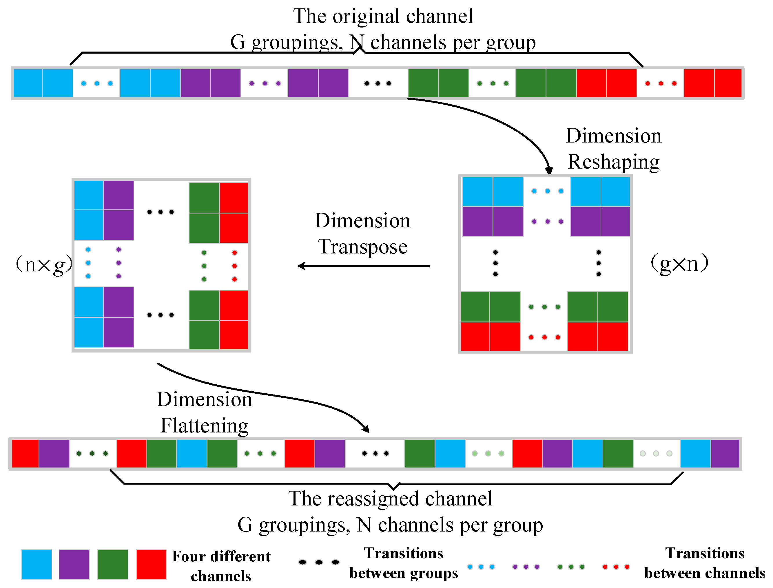
3.1. Self-Compensation Convolution

Aiming at the problem that the parameters of traditional convolution increase sharply when the number of filters is large (the number of filters commonly used is 512 or 1024), a self-compensated convolution was proposed from the perspective of reducing the number of filters. Figure 1 shows the convolution process of traditional convolution and self-compensation convolution, respectively.

As shown in Figure 2, the output features $Y\in {ℝ}^{h\times w\times 2c}$ of the traditional convolution are obtained by the input features $X\in {ℝ}^{\mathrm{h}\times w\times c}$. The convolution process can be represented asL

$$Y=X\ast f$$

(1)

In Formula (1), $\ast$ represents the convolution operation. For the filter $f\in {ℝ}^{k\times k\times c}$, $c$ is the number of channels and $k\times k$ is the kernel size of the convolution filter. $h$ and $w$ are the height and width of the input features, respectively. The number of calculations required for this convolution process is $k\times k\times c_{}\times 2c_{}$, which is usually huge because the number of channels c is large (for example, 512 or 1024). A large number of filters cause the network to run slowly. Aimed at the problem that the network slows down due to the large number of filters of the traditional convolution process, we proposed a self-compensation convolution without increasing the computational effort, as shown in Figure 2. The core idea of this convolution is to first reduce the number of filters to obtain a set of convoluted features, then compensate the convoluted channels with the original input to obtain the same output features as the traditional convolution, and finally reassign the feature maps. Because the original inputs are utilized to compensate the features obtained from those small numbers of filters, we called it self-compensating convolution. Self-compensated convolution mainly consists of two parts. In the first convolution process, the number of filters is half the number of input channels. In the second convolution process, the number of filters is equal to the number of input channels. Compared with the number of filters that directly use twice the number of input channels in traditional convolution, the twice small convolution kernel of self-compensated convolution has great advantages. It improves the running speed of the network without increasing the amount of calculation, and achieves satisfactory classification accuracy.

The process of self-compensated convolution is as follows. First, the input features are convoluted with a set of reduced convolution kernels to obtain some features $F_{conv1}(x)\in {ℝ}^{h\times w\times \frac{1}{2}c}$. $F_{conv1}(x)$ can be expressed by Formula (2):

$$F_{conv1}(x)=X\ast f$$

(2)

In Formula (2), $f\in {ℝ}^{k\times k\times \frac{1}{2}c}$ is the convolution kernel and $k\times k$ is the size of the convolution kernel. To obtain a large receptive field, $k$ is set to 5.

Next, the feature maps $F_{conv1}(x)\in {ℝ}^{h\times w\times \frac{1}{2}c}$ and the original input $X\in {ℝ}^{\mathrm{h}\times w\times c}$ are channel fused to obtain the fused features $U\in {ℝ}^{h\times w\times \frac{3}{2}c}$. $U$ can be represented by Formula (3):

$$U={\displaystyle \sum _{i=1}^C{\displaystyle \sum _{j=1}^{\frac{C}{2}}([F_{conv1},X])}}=(u_1^{H\times W},u_2^{H\times W},\dots ,u_{\raisebox{1ex}{$3C$}\!\left/ \!\raisebox{-1ex}{$2$}\right.}^{H\times W})$$

(3)

In Formula (3), $F_{conv1}=[f_1^{H\times W},f_2^{H\times W},\dots ,f_{C/2}^{H\times W}]\in {ℝ}^{H\times W\times \frac{C}{2}}$, $f_i^{H\times W}$ represents the feature with size $H\times W$ in the $i$-th channel. $X=[x_1^{H\times W},x_2^{H\times W},\dots ,x_C^{H\times W}]\in {ℝ}^{H\times W\times C}$, $x_i^{H\times W}$ represents the feature with size $H\times W$ in the $i$-th channel. In Formula (3), ${\displaystyle \sum _{i=1}^C{\displaystyle \sum _{j=1}^{C/2}([F_{conv1},X])}}$ indicates that feature $F_{conv1}$ and the feature $X$ are concatenated channel by channel. $u_i^{H\times W}$ represents the feature with size $H\times W$ in the $i$-th channel after fusion.

Then, after channel reassignment with fused features $U\in {ℝ}^{h\times w\times \frac{3}{2}c}$, the feature maps $X_1\in {ℝ}^{\mathrm{h}\times w\times \frac{3}{2}c}$ are obtained. Following, $X_1$ is convoluted with $f_1$ to obtain $F_{conv2}(x)\in {ℝ}^{h\times w\times c}$, as shown in Formula (4):

$$F_{conv2}(x)=X_1\ast f_1$$

(4)

In Formula (4), $f_1\in {ℝ}^{k\times k\times c}$ is the convolution kernel and $k\times k$ is the size of the convolution kernel. To reduce the computational load of the model, set $k=3$.

By channel fusion of feature maps $F_{conv2}(x)\in {ℝ}^{h\times w\times c}$ and original input $X\in {ℝ}^{\mathrm{h}\times w\times c}$, the new feature maps $T\in {ℝ}^{H\times W\times 2C}$ are obtained, which can be represented by Formula (5):

$$T={\displaystyle \sum _{i=1}^c{\displaystyle \sum _{j=1}^c([F_{conv2},X])}}=(t_1^{H\times W},t_2^{H\times W},\dots ,t_{2C}^{H\times W})$$

(5)

In Formula (5), ${\displaystyle \sum _{i=1}^C{\displaystyle \sum _{j=1}^C([F_{conv2},X])}}$ indicates that the feature $F_{conv2}$ and the feature $X$ are concatenated channel by channel. $t_i^{H\times W}$ represents the feature with size $H\times W$ in the $i$-th channel after fusion. Finally, after channel reassignment with feature maps $T$, the final output $Y\in {ℝ}^{\mathrm{H}\times W\times 2C}$ is obtained.

To accelerate the network, the batch normalization (BN) was adopted after each convolution. Assuming the image set input to a channel was $\gamma =[x_1\dots x_n]\in {ℝ}^{N\times H\times W}$, the mean ${\mu }_{\gamma }$ and variance ${\sigma }_{\gamma }^2$ of batch data were calculated according to Formulas (6) and (7), respectively, and then the data range of [0, 1] was obtained by normalization processing, as shown in Formula (8). Here, $\epsilon$ is a positive number with a smaller value to avoid a denominator of zero, and finally the normalized data ${\widehat{x}}_i$ is scale transformed and shift by Equation (9). Because the data ${\widehat{x}}_i$ after normalization would be restricted to a normal distribution, resulting in the reduced expression ability of the network, two parameters, $\lambda$ and $\beta$, were introduced to scale transform and shift the normalized data ${\widehat{x}}_i$. Multiplying ${\widehat{x}}_i$ by $\lambda$ adjusts the magnitude of the value and then adding $\beta$ increases the shift to obtain $y_i$. Here $\lambda$ is the scale factor and $\beta$ is the shift factor. Formulas (6)–(9) are represented as follows:

$${\mu }_{\gamma }=\frac{1}{n}{\displaystyle \sum _{i=1}^n{x}_i}$$

(6)

$${\sigma }_{\gamma }^2=\frac{1}{n}{\displaystyle \sum _{i=1}^n(x_i}-{\mu }_{\gamma }{)}^2$$

(7)

$$\stackrel{\wedge }{x_i}=\frac{x_i-{\mu }_{\gamma }}{\sqrt{{\sigma }_{\gamma }^2+\epsilon }}$$

(8)

$$y_i=\lambda x_i+\beta =B{N}_{\lambda ,\beta }(x_i)$$

(9)

After the fusion of shallow features and deep features, in order to ensure that the information of different channels can be fully fused and exchanged, the features of the compensated channel were reassigned. The reassigned process of features of each channel is shown in Figure 3. As shown in Figure 3, channel reassignment is a process of fully interacting with different channels, assuming a convolution layer is divided into $g$ groups with $n$ channels for each group, i.e., there are $g\times n$ channels in total. The channel dimension was first reshaped to $(g\times n)$, then transposed to $(n\times g)$, and finally flattened to obtain the output result after reassignment. In addition, in order to verify the impact of channel reassignment after the fusion of shallow features and deep features on network performance, a detailed experimental comparison is carried out in the discussion section.

3.2. Self-Compensating Bottleneck Module

With the deepening of the network, the extracted features contain more semantic information, which is more conducive to improve the performance of classification. However, the deepening of the network not only brings more parameters, but also makes the network training more difficult. In order to solve this problem, we proposed a self-compensating bottleneck module (SCBM) based on self-compensating convolution, as shown in Figure 4. SCBM not only reduces the amount of parameters, but also increases the depth of the network and further reduces the difficulty of training. $X\in {ℝ}^{H\times W\times C}$ represents the input feature and $Y\in {ℝ}^{H\times W\times C^{\ast }}$ represents the output feature. First, the dimension of the input feature $X$ is reduced by 1 × 1 convolution to obtain ${\Upsilon }^{1,P}(X)$; ${\Upsilon }^{1,P}$ represents the first 1 × 1 convolution in the bottleneck structure. Because the use of activation function leads to the loss of feature information when the dimension is low, the activation function is not used after 1 × 1 convolution for dimension reduction. The reduced-dimension feature passes through two consecutive 3 × 3 self-compensating convolution to obtain $\widehat{Y}$, $\widehat{Y}={\Upsilon }^{2,S}{\Upsilon }^{1,S}{\Upsilon }^{1,P}(X)$, ${\Upsilon }^{i,S}$ represents the $i$th 3 × 3 self-compensation convolution. The two continuous 3 × 3 self-compensation convolutions can not only extract rich spatial information, but also increase the width of the bottleneck structure. The wider short connection is conducive to more information transmit from input $X$ to output $Y$. Then, 1 × 1 convolution is adopted to increase the dimension of the features to obtain $\tilde{Y}$, $\tilde{Y}={\Upsilon }^{2,P}{\Upsilon }^{2,S}{\Upsilon }^{1,S}{\Upsilon }^{1,P}(X)$; ${\Upsilon }^{2,P}$ represents the second 1 × 1 convolution in the bottleneck structure. Finally, the input feature $X$ and the output feature $\tilde{Y}$ are short connected in the channel dimension to obtain $Y$, $Y=\tilde{Y}\odot X$; $\odot$ represents a short connection in the channel dimension. Using the channel dimension shortcut cannot be affected by the feature input and output size, which is more conducive to deploying the bottleneck module in the whole model. The whole structure can be expressed by Formulas (10) and (11):

$$\tilde{Y}={\Upsilon }^{2,P}{\Upsilon }^{2,S}{\Upsilon }^{1,S}{\Upsilon }^{1,P}(X)$$

(10)

$$Y=\tilde{Y}\odot X$$

(11)

Table 1. Operational description of the proposed residual module.

Input Dimension	Operator	Output Dimension
$H\times W\times C$	$1\times 1$ Conv	$H\times W\times (C/4)$
$H\times W\times (C/4)$	$3\times 3$ SSC	$H\times W\times (C/4)$
$H\times W\times (C/4)$	$3\times 3$ SSC	$H\times W\times (C/4)$
$H\times W\times (C/4)$	$1\times 1$ Conv	$H\times W\times C^{\ast }$

details the feature size changes of the self-compensating bottleneck module from input $X$ to output $Y$. $C/4$ in Table 1 represents the dimension of the reduced channel, $H$, $W$, $C$, and $C^{\ast }$ represents the height, width, number of input and output channels of the feature, respectively.

3.3. Self-Compensating Convolution Neural Network

Based on the proposed self-compensation bottleneck module, a lightweight, modular self-compensated convolutional neural network (SCCNN) for remote sensing image classification is proposed. The network model structure is shown in Figure 5. The network is mainly stacked orderly by self-compensation bottleneck modules with different numbers of channels. The specific process is as follows. Firstly, the shallow features of the input feature maps are extracted by two consecutive traditional convolution operations. Then these shallow features are sent to six self-compensation bottleneck modules in succession. In order to prevent over-fitting, a maximum pooling layer was added after the self-compensation bottleneck module to down-sample the features, preserving the main features of the feature map while reducing the amount of parameters and computation of the network, thus effectively avoiding over-fitting. Assuming that $x_{nxy}$ represents the sample with coordinate $(x,y)$ in rectangular area $R_{ij}$, $f_{nxy}$ represents the maximum pooled value in rectangular area $R_{ij}$ related to the $i$-th features. The expression of $f_{nxy}$ is shown in Formula (12):

$$f_{nxy}=\underset{(x,y)\in R_{ij}}{\max }{x}_{nxy}$$

(12)

Finally, the feature maps are used for classification after global average pooling.

4. Experiment and Results

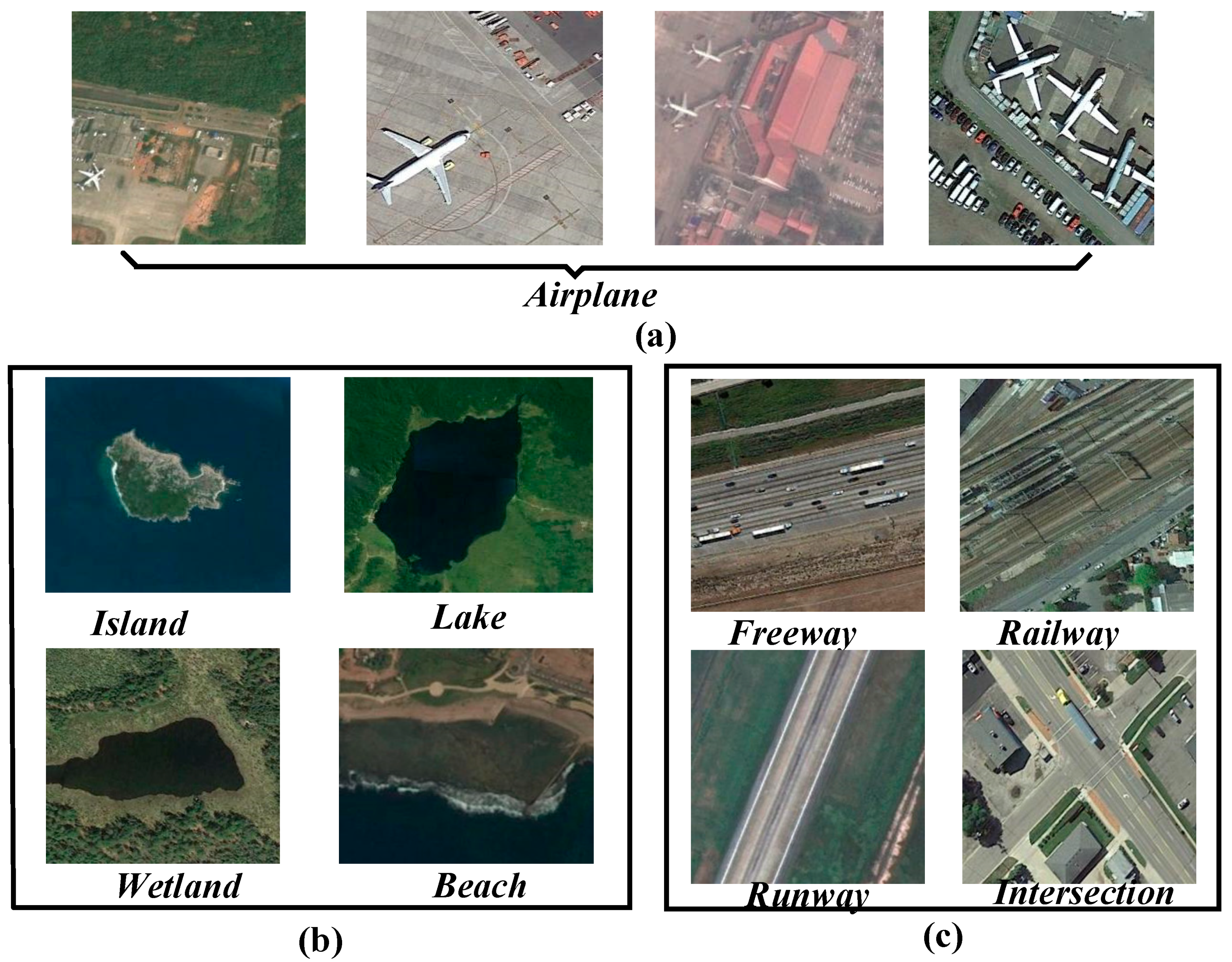
In this section, some indicators are adopted to evaluate the proposed network model. The experiments are conducted on six more challenging datasets, and the proposed method is compared with some state-of-the-art classification methods. In order to ensure the reliability of the experimental results, all methods are carried out with the same super parameters and on the same computer. The experimental results show that the proposed method can classify remote sensing scene images more effectively and has obvious advantages in terms of parameter quantity and running speed.

4.1. Datasets

Some experiments were performed on six commonly used datasets. The datasets were UCM21 [30], RSSCN7 [31], AID [32], NWPU-RESISC45 [33], WHU-RS19 [34], and SIRI-WHU [35], respectively. In

Table 2. Comparison of six datasets.

Datasets	Number of Images in Each Category	Number of Categories	Total Number of Images	Spatial Resolution (m)	Image Size
UCM21	100	21	2100	0.3	256 × 256
RSSCN7	400	7	2800	-	400 × 400
AID	200~400	30	10,000	0.5~0.8	600 × 600
NWPU45	700	45	31,500	~30–0.2	256 × 256
WHU-RS19	~50	19	1005	0.5	600 × 600
SIRI-WHU	200	12	2400	2	200 × 200

, the number of images, the number of scene categories, the total number of images, the spatial resolution of images, and the image size of six datasets are compared. Some sample images of datasets UCM21, RSSCN7, SIRI-WHU, WHU-RS19, AID, and NWPU45 are shown in Figure A1, Figure A2, Figure A3, Figure A4, Figure A5 and Figure A6 in Appendix A, respectively.

4.2. Setting of the Experiments

A stratified sampling method was adopted to partition the dataset to avoid the risk of sampling bias. In addition, random seeds were set during the stratified sampling to ensure that the same images were chosen for each experiment. To increase the reliability of the experimental results, we used the average value as the final evaluation result after 10 experiments at each training proportion. For the UCM21 dataset, the training proportion was set to 80%, for RSSCN7 dataset to 50%, for AID dataset to 20% and 50%, and for NWPU45 dataset to 10% and 20%, respectively. For the WHU-RS19 dataset, the training proportion was set to 40% and 60%, respectively. The SIRI-WHU dataset training proportions were set to 50% and 80%, respectively. The initial learning rate was set to 0.01. In addition, an automatic attenuation mechanism of learning rate was adopted. The momentum during training was 0.9, the batch size was set to 16. The experiments were conducted on a computer with an AMD Ryzen 7-4800H CPU, and RTX2060 GPU, and 16 GB of RAM.

4.3. Visual Analysis of the Model

To evaluate the validity of the proposed method, some experiments were performed on two datasets, RSSCN7 and UCM21, evaluated by the T-distributed stochastic neighbor embedding visualization method (T-SNE). By mapping high-dimensional data to two-dimensional space and visualizing the classification results with scattering distribution, the classification performance of the proposed model was evaluated very well. The results of T-SNE visualization analysis on different datasets are shown in Figure 6. As can be seen in Figure 6, the proposed method can effectively overcome the problems of large intra-class differences and inter-class similarities of remote sensing scene images, distinguish each class well, and can provide excellent classification performance.

In addition, on UCM21 dataset with train: test = 8:2, some random classification experiments were performed with the proposed method. The results of the experiment are shown in Figure 7. From Figure 7, it can be seen that the predicted scenario and the real scenario are basically the same, with all of them reaching more than 99% confidence, and some of them reaching 100%.

4.4. Comparison with Advanced Methods

In the experiments, the proposed method was compared with some of the most recently proposed remote sensing scene classification methods under the same experimental conditions. The overall accuracy (OA), confusion matrix, and number of parameters were used as the evaluation indicators for quantitative analysis. Firstly, some experiments were performed on the UCM21 dataset with training: test = 8:2. The experimental results are listed in

Table 3. Performance comparison of the proposed model with some advanced methods on the UCM21 dataset.

The Network Model	OA (%)	Number of Parameters
Siamese CNN [36]	94.29	-
Siamese ResNet50 with R.D method [37]	94.76	-
Bidirectional adaptive feature fusion method [38]	95.48	130 M
Multiscale CNN [39]	96.66 ± 0.90	60 M
VGG_VD16 with SAFF method [40]	97.02 ± 0.78	15 M
Variable-weighted multi-fusion method [41]	98.56 ± 0.23	15 M
ResNet + WSPM-CRC method [42]	97.95	23 M
Skip-connected CNN [43]	97.98 ± 0.56	6 M
VGG16 with MSCP [44]	98.36 ± 0.58	-
Gated bidirectiona + global feature method [45]	98.57 ± 0.48	138 M
Feature aggregation CNN [46]	98.81 ± 0.24	130 M
Aggregated deep fisher feature method [47]	98.81 ± 0.51	23 M
Discriminative CNN [48]	98.93 ± 0.10	130 M
VGG16-DF method [49]	98.97	130 M
Scale-Free CNN [50]	99.05 ± 0.27	130 M
Inceptionv3 + CapsNet method [51]	99.05 ± 0.24	22 M
Positional context aggregation method [52]	99.21 ± 0.18	28 M
LCNN-BFF method [53]	99.29 ± 0.24	6.2 M
DDRL-AM method [54]	99.05 ± 0.08	-
Coutourlet CNN [55]	99.25 ± 0.49	12.6 M
SE-MDPMNet [56]	99.09 ± 0.78	5.17 M
ResNet50 [57]	98.76 ± 0.15	25.61 M
Multiple resolution BlockFeature method [58]	94.19 ± 1.5	-
LPCNN [59]	99.56 ± 0.58	5.6 M
SICNN [60]	98.67 ± 0.82	23 M
Pre-trained-AlexNet-SPP-SS [61]	98.99 ± 0.48	38 M
SRSCNN [62]	97.62 ± 0.28	-
DCA by addition [63]	99.46 ± 0.37	45 M
Two-stream deep fusion Framework [64]	99.35 ± 0.3	6 M
Semi-supervised representation learning method [65]	94.05 ± 1.2	210 M
Proposed	99.76 ± 0.05	0.49 M

. It can be seen that the OA accuracy of the proposed model was 99.76%, 5.47% higher than that of Siamese CNN method [36], and 5% higher than that of Siamese ResNet50 with R.D method [37]. It is worth noting that our method had only 0.49 M parameters. Here, M refers to MByte, which was used to measure the amount of model parameters. In other words, the proposed method achieved the best classification performance on UCM21 datasets with the least number of parameters.

Next, some experiments were performed on the RSSCN7 dataset with training: test = 5:5, and the proposed method was compared with some advanced methods. The experimental results are shown in

Table 4. Performance comparison of the proposed model with some advanced methods on the RSSCN7 dataset.

The Network Model	OA (%)	Number of Parameters
VGG16 + SVM method [32]	87.18	130 M
Variable-weighted multi-fusion method [41]	89.1	53 M
ResNet + SPM-CRC method [42]	93.86	23 M
Aggregated deep fisher feature Method [48]	95.21 ± 0.50	23 M
LCNN-BFF method [53]	94.64 ± 0.21	6.2 M
Coutourlet CNN [55]	95.54 ± 0.17	12.6 M
SE-MDPMNet [56]	92.64 ± 0.66	5.17 M
Proposed	97.21 ± 0.32	0.49 M

. As can be seen from Table 4, the proposed method achieved 97.21% classification accuracy with 0.49 M parameters, which had the highest classification accuracy and the fewest parameters among all the comparison methods. The classification accuracy of the proposed method was 2% higher than the aggregated deep fisher feature method [48] and 2.57% higher than the LCNN-BFF method [53].

Table 5. Performance comparison of the proposed model with some advanced methods on the AID30 dataset.

The Network Model	OA (20/80%)	OA (50/50%)	Number of Parameters
Bidirectional adaptive feature fusion method [38]	-	93.56	130 M
VGG_VD16 with SAFF method [40]	90.25 ± 0.29	93.83 ± 0.28	15 M
Skip-connected CNN [43]	91.10 ± 0.15	93.30 ± 0.13	6 M
Gated bidirectiona method [45]	90.16 ± 0.24	93.72 ± 0.34	18 M
Gated bidirectiona + global feature method [45]	92.20 ± 0.23	95.48 ± 0.12	138 M
Feature aggregation CNN [46]	-	95.45 ± 0.11	130 M
Discriminative CNN [48]	85.62 ± 0.10	94.47 ± 0.12	60 M
LCNN-BFF method [53]	91.66 ± 0.48	94.64 ± 0.16	6.2 M
ResNet50 [57]	92.39 ± 0.15	94.69 ± 0.19	25.61 M
Fine-tuning method [32]	86.59 ± 0.29	89.64 ± 0.36	130 M
Proposed	93.15 ± 0.25	97.31 ± 0.10	0.49 M

lists the experimental results on AID datasets with training: test = 2:8 and training: test = 5:5, respectively. It can be seen that our method achieved the best classification performance when the training ratio was 20%. The proposed model achieved a classification accuracy of 93.15%, 0.76% higher than that of ResNet50 [57], and 0.95% higher than that of gated bidirectiona + global feature method [45]. When the training proportion was 50%, our method also achieved the best classification accuracy. The classification accuracy of the proposed method was 1.83% higher than that of the gated bidirectiona + global feature method [45]. This further proves that our method has stronger feature representation ability and can learn more discriminatory features under the same conditions.

Table 6. Performance comparison of the proposed model with some advanced methods on the SIRI-WHU dataset.

The Network Model	OA (50/50%)	OA (80/20%)	Number of Parameters
DMTM [35]	91.52	-	-
Siamese ResNet_50 [36]	95.75	97.50	-
Siamese AlexNet [36]	83.25	88.96	-
Siamese VGG-16 [36]	94.50	97.30	-
Fine-tune MobileNetV2 [56]	95.77 ± 0.16	96.21 ± 0.31	3.5 M
SE-MDPMNet [56]	96.96 ± 0.19	98.77 ± 0.19	5.17 M
LPCNN [59]	-	89.88	-
SICNN [60]	-	93.00	-
Pre-trained-AlexNet-SPP-SS [61]	-	95.07 ± 1.09	-
SRSCNN [62]	93.44	94.76	-
Proposed	98.08 ± 0.45	99.37 ± 0.26	0.49 M

lists the experimental results on SIRI-WHU dataset with training: test = 5:5 and training: test = 8:2. It can be seen that the proposed method was superior to all comparison methods. When the training proportions were 50% and 80%, the average classification accuracies of the proposed method were 98.08% and 99.37%, which were 1.12% and 0.6% higher than that of SE-MDPMNET method, and 2.31% and 3.16% higher than that of the fine-tune MobileNetV2 method with similar parameters. This proves that the proposed method is effective for the classification of remote sensing scene images.

Some experiments were carried out on WHU-RS19 dataset with training: test = 4:6, and training: test = 6:4. The results are shown in

Table 7. Performance comparison of the proposed model with some advanced methods on the WHU-RS19 dataset.

The Network Model	OA (40/60%)	OA (60/40%)	Number of Parameters
CaffeNet [32]	95.11 ± 1.20	96.24 ± 0.56	60.97 M
VGG-VD-16 [32]	95.44 ± 0.60	96.05 ± 0.91	138.36 M
GoogLeNet [32]	93.12 ± 0.82	94.71 ± 1.33	7 M
Fine-tune MobileNetV2 [56]	96.82 ± 0.35	98.14 ± 0.33	3.5 M
SE-MDPMNet [56]	98.46 ± 0.21	98.97 ± 0.24	5.17 M
DCA by addition [63]	-	98.70 ± 0.22	-
Two-stream deep fusion Framework [64]	98.23 ± 0.56	98.92 ± 0.52	-
TEX-Net-LF [45]	98.48 ± 0.37	98.88 ± 0.49	-
Proposed	98.65 ± 0.45	99.51 ± 0.15	0.49 M

. For different numbers of training samples, the proposed method performed better than all the methods used for comparison. When the training proportion was 40%, the classification accuracy of the proposed method was 98.65%, 0.17% higher than that of TEX-Net-LF [45], and 0.19% higher than that of SE-MDPMNET [56]. When the training proportion was 60%, the classification accuracy of the proposed method was 99.51%, 0.59% higher than that of the two-stream deep fusion framework [64], and 0.54% higher than that of SE-MDPMNET [56]. When the training proportions were 40% and 60%, compared with fine-tune MobileNetV2 [56] method with the least parameters, the proposed method had 1.83% and 1.73% higher classification accuracies, respectively.

Finally, the performance of the method was further evaluated on the NWPU45 dataset. The dataset was divided into training: test = 1:9 and training: test = 2:8. The experiments were carried out and the results are shown in

Table 8. Performance comparison of the proposed model with some advanced methods on the NWPU45 dataset.

The Network Model	OA (10/90%)	OA (20/80%)	Number of Parameters
VGG_VD16 with SAFF method [40]	84.38 ± 0.19	87.86 ± 0.14	15 M
Skip-connected CNN [43]	84.33 ± 0.19	87.30 ± 0.23	6 M
Discriminative with AlexNet [48]	85.56 ± 0.20	87.24 ± 0.12	130 M
Discriminative with VGG16 [48]	89.22 ± 0.50	91.89 ± 0.22	130 M
VGG16 + CapsNet [51]	85.05 ± 0.13	89.18 ± 0.14	130 M
LCNN-BFF method [53]	86.53 ± 0.15	91.73 ± 0.17	6.2 M
Contourlet CNN [55]	85.93 ± 0.51	89.57 ± 0.45	12.6 M
ResNet50 [57]	86.23 ± 0.41	88.93 ± 0.12	25.61 M
InceptionV3 [57]	85.46 ± 0.33	87.75 ± 0.43	45.37 M
Fine-tuning method [32]	87.15 ± 0.45	90.36 ± 0.18	130 M
Proposed	92.02 ± 0.50	94.39 ± 0.16	0.49 M

. When the proportion of training was 10% and 20%, the accuracy of our proposed method was 92.02% and 94.39%, respectively, which was 2.8% and 2.5% higher than that of the discriminative with VGG16 [48] method which achieved the highest accuracy. When training: test = 1:9, our method had a 7.69% higher classification accuracy than the lightweight skip-connected CNN [43]. When training: test = 2:8, our method had a 7.09% higher classification accuracy than the lightweight skip-connected CNN [43]. This shows that for images with high interclass similarity and high intraclass difference, the proposed method can extract more discriminative features with lower parameters.

4.5. Performance Evaluation of the Proposed SCCNN Method

In this section, the performance of the proposed method was evaluated by using the confusion matrix evaluation index. Figure 8 is the confusion matrix for the proposed method on the UCM21 dataset. From the confusion matrix, we can see that the proposed method achieved 100% correct classification for almost all scenes. This further demonstrates that the proposed method performs well on UCM21 datasets.

A confusion matrix derived from the proposed method on the RSSCN7 dataset is shown in Figure 9. As shown in Figure 9, the ‘Forest’ scene achieved an optimal classification accuracy of 100%, which meant that there were large intraclass differences in this scene. On the other hand, the ‘Grass’ scene had a poor classification accuracy of 92%. This was due to the large class similarity between ‘Grass’ and ‘Field’, which resulted in some grass being misclassified into the field category. Nevertheless, the proposed method still provides a good classification of grasslands and fields.

Figure 10 is a confusion matrix obtained by the proposed method on the AID datasets. From Figure 10, it can be seen that, except for the ‘School’ scene, the classification accuracy of all the scenarios reached more than 90%, of which the classification accuracy of ‘Meadow’, ‘Sparse Residential’, and ‘Viaduct’ was 100%. For the ‘School’ scene, the classification accuracy was at least 86%. The three scenarios of ‘School’, ‘Commercial’, and ‘Industrial’ are the most confusing because they have similar structures, such as buildings, plants, and ponds. Nevertheless, compared with other advanced classification methods, the proposed method still provides higher classification accuracy.

Figure 11 is a confusion matrix obtained by the proposed method on a SIRI-WHU dataset with a training proportion of 80%. It can be seen that ten scenes were correctly classified, and the incorrectly classified scenes included ‘Commercial’ and ‘Residential’, with classification accuracy of 98% for both scenarios. Some ‘Residential’ scenes were incorrectly classified as ‘Industrial’ because they include some buildings and grasslands, resulting in very high class similarities. Nevertheless, the proposed method still shows good classification performance.

Figure 12 shows the confusion matrix of the proposed method with training: test = 6:4 on the WHU-RS19 dataset. Except for the ‘Port’ and ‘Pond’, the other scenarios were fully recognized. The most confusing scenarios were those of ‘Port’ and ‘Pond’. Because both scenarios contain the water, ‘Pond’ can easily be misclassified as ‘Port’. Nevertheless, the proposed method still achieves good classification results for these scenarios.

The confusion matrix when the training ratio was 20% is shown in Figure 13. As can be seen from Figure 13, on the NWPU45 dataset with training: test = 2:8, the classification accuracy of all scenarios except the ‘Palace’ scenario reached more than 90%. In addition, the classification accuracy of ‘Palace’ and ‘Church’ scenes with high degree of confusion also reached 89% and 90%, respectively. This further verifies that our method also performs well on more challenging datasets.

4.6. Comparison of Model Running Time

To further evaluate the advantage of our method in terms of speed, the proposed method was tested on UCM21 datasets using the ATT (average training time) evaluation index and then comparing it with the advanced methods. ATT refers to the average training time required by a model to process an image. Because the value of ATT is closely related to the configuration of the computer, all methods used for comparison were run on the same computer as the proposed method. The experimental comparison results are shown in

Table 9. ATT comparison of the proposed model with some advanced methods on UC datasets.

The Network Model	Time Required to Process Each Image (s)
Siamese ResNet_50 [36]	0.053
Siamese AlexNet [36]	0.028
Siamese VGG-16 [36]	0.039
LCNN-BFF [53]	0.029
GBNet + global feature [45]	0.052
GBNet [45]	0.048
Proposed	0.014

.

As can be seen from Table 9, in the same case, it took the least time for the proposed method to process one image. It was 0.014 s faster than that of the Siamese AlexNet [36] method and 0.015 s faster than that of the LCNN-BFF [53] method. Compared with Siamese ResNet_50 [36], Siamese VGG-16 [36], GBNet + global feature [45], and GBNet [45], the running time was reduced by 0.039, 0.025, 0.038, and 0.034 s, respectively. It is worth noting that the ATT value is smaller if the experiments are performed with a higher-configuration device.

4.7. Comparison of Computational Complexity of Models

In this section, we used the floating-point operations (FLOPs) value to compare model performance on RSSCN datasets. Floating-point operations (FLOPs) represent the complexity of the model, and a smaller value indicates that the proposed model is lighter. The comparison results are shown in

Table 10. Evaluation of some models’ complexity.

The Network Model	OA (%)	Number of Parameters	FLOPs
LCNN-BFF [53]	94.64	6.1 M	24.6 M
GoogLeNet [32]	85.84	7 M	1.5 G
CaffeNet [32]	88.25	60.97 M	715 M
VGG-VD-16 [32]	87.18	138 M	15.5 G
Fine-tune MobileNetV2 [56]	94.71	3.5 M	334 M
SE-MDPMNet [56]	92.64	5.17 M	3.27 G
Contourlet CNN [55]	95.54	12.6 M	2.1 G
Proposed	97.21	0.49 M	1.9 M

.

From Table 10, we can see that our proposed method achieved the highest classification accuracy compared with all the comparison methods with 0.49 M parameters. In addition, the FLOPs value of the proposed method was the smallest and the computational complexity was the lowest. Compared with the lightweight network fine-tune MobileNetV2 [56], the accuracy was improved by 2.5%, the FLOPs value was decreased by 332 M, the accuracy was improved by 2.57%, and the FLOPs value was decreased by 23 M compared with the lightweight network LCNN-BFF [53]. This proves that the proposed method is a lightweight convolution network with good performance.

5. Discussion

In this section, the following two parts are discussed. Firstly, we compared the performance of the proposed self-compensated convolution (SCC) with that of the traditional convolution. Secondly, the impact of channel reassignment after the fusion of shallow and deep features on the performance of the model is discussed. Some experiments were performed on NWPU and AID datasets under the same experimental conditions, where, training: test = 2:8 for the NWPU dataset and training: test = 5:5 for the AID dataset. The number of parameters, overall accuracy (OA), floating-point operations (FLOPs), Kappa coefficient, and average training time (ATT) were used for various comparisons.

We replaced the two consecutive self-compensating convolutions of the self-compensating bottleneck module (SCBM) in Figure 4 with the traditional convolution bottleneck module (CBM), which is shown in Figure 14. The comparison of experimental results is listed in

Table 11. Performance comparison between the self-compensated convolution and the traditional convolution.

The Network Model	OA (%)		Kappa (%)		ATT		FLOPs		Number of Parameters
	AID	NWPU	AID	NWPU	AID	NWPU	AID	NWPU
SCBM	97.31	94.39	97.05	93.68	0.045 s	0.093 s	1.9 M	2.0 M	0.49 M
CBM	95.56	92.45	94.64	91.49	0.135 s	0.245 s	3.3 M	3.4 M	0.85 M

. As can be seen from Table 11, the proposed self-compensation convolution had great advantages in classification performance compared with the traditional convolution. In terms of evaluation index, with ‘FLOPs’ measuring the computational complexity of the model and the evaluation index ‘number of parameters’ measuring the size of the model, both the proposed SCBM method and CBM can realize lightweight networks. However, the FLOPs and the number of parameters of the proposed SCBM method were 2.4 and 0.36 M lower than that of CBM, respectively. The SCBM method had advantages in model complexity. This is because the self-compensation convolution in the self-compensation bottleneck module can reduce the complexity of the model without increasing the number of parameters. Self-compensation convolution integrates shallow features into deep complex features by reducing the number of filters and using input features to compensate the features after reduced dimension convolution, which helps to improve the speed and classification accuracy of the model. For the AID dataset with training: test = 5:5, the OA value of the proposed SCBM method reached 97.31%, which is 1.75% higher than that of CBM. The Kappa coefficient of SCBM was 97.05%, which is 2.41% higher than that of CBM. In addition, in terms of model speed, the ATT of the proposed SCBM method was 0.09 s shorter than that of the CBM method. When the experiment was carried out on the NWPU45 dataset with training: test = 2:8, the classification accuracy of the proposed SCBM method was 94.39%, and the Kappa value was 93.68%, which is 1.94% and 2.19% higher than that of CBM method, respectively. These experimental results prove that the proposed SCBM method is a lightweight method and can provide high classification accuracy.

In order to intuitively show the feature extraction ability of SCBM and CBM, the grad cam visualization method was adopted to evaluate the two methods. In this experiment, some remote sensing scene images—‘Airplane’, ‘Dense residential’, ‘Buildings’, ‘Chaparral’, ‘Forests’, ‘Beach’, ‘Baseball diamond’, and ‘Agricultural’—in the UC dataset were randomly selected. The visualization results of the two methods are shown in Figure 15.

From the visualization results in Figure 15, it can be seen that the proposed SCBM method can extract feature information more effectively. For two scenarios, ‘Airplane’ and ‘Baseball diamond’, the proposed SCBM method extracted the key features of the scenario, while the feature information extracted by the CBM method was offset. For other scenarios such as ‘Dense residential’ and ‘Buildings’, the proposed method also extracted a larger area of interest for the target, which is conducive to the improvement of classification accuracy. This is because the wider residual connection between input and output in the self-compensation bottleneck module helps to transmit more shallow location information to the deep layer of the network, so that the output features not only contain rich semantic features, but also increase more location information, which can have a greater coverage of the target region.

Next, the impact of channel reassignment on the performance of the network model is verified by some experiments. The network without the channel reassignment operation in self-compensation convolution is called convolution network (CN). The results under the same experimental conditions are shown in

Table 12. Influence of channel reassignment on network model performance after channel fusion.

The Network Model	OA (%)		Kappa (%)		ATT		FLOPs		Number of Parameters
	AID	NWPU	AID	NWPU	AID	NWPU	AID	NWPU
SCCNN	97.31	94.39	97.05	93.68	0.045 s	0.093 s	1.99 M	2.03 M	0.49 M
CN	96.41	93.29	96.35	93.08	0.045 s	0.093 s	1.99 M	2.03 M	0.49 M

. It can be seen from Table 12 that the classification accuracy can be improved by about 1% by using the channel redistribution operation after channel fusion, because the channel redistribution operation can exchange information of the features among different groups and improve the representation ability of the features. In addition, it can be seen from Table 12 that the use of channel redistribution operation has no impact on the running time of the network model. It is worth noting that, compared with the traditional CBM method in Table 11, the classification accuracy of self-compensated convolution without channel reassignment was even higher than that of traditional convolution, which further verifies the superiority of self-compensation convolution.

6. Conclusions

In this paper, in order to solve the problem that the network running speed slows down when the number of traditional convolution filters is large, a self-compensation convolution (SCC) was proposed. The self-compensation convolution can achieve better performance than the traditional convolution while reducing the number of parameters. Then, in order to solve the problem of training difficulty caused by network deepening, a self-compensation bottleneck module (SCBM) was proposed based on self-compensation convolution. The self-compensation bottleneck module can deepen the network and reduce the difficulty of network training. Finally, a lightweight and modular self-compensation convolution neural network (SCCNN) was built through the self-compensation bottleneck module. A large number of experiments were carried out on six datasets with different training ratios, and the experimental results show the effectiveness of the proposed method. The next step of work is to find a more effective method for feature extraction and further improve the classification accuracy of remote sensing scene images.

References

1. Krizhevsky, A.; Sutskever, I.; Hinton, G. Imagenet classification with deep convolutional neural networks. Adv. Neural Inf. Process. Syst. 2012, 25, 1097–1105. [Google Scholar] [CrossRef]
2. Han, K.; Guo, J.; Zhang, C.; Zhu, M. Attribute-aware attention model for fifine-grained representation learning. In Proceedings of the 26th ACM International Conference on Multimedia (MM’18), Seoul, Korea, 22–26 October 2018; pp. 2040–2048. [Google Scholar]
3. Ren, S.; He, K.; Girshick, R.; Sun, J. Faster R-CNN: Towards real-time object detection with region proposal networks. Adv. Neural Inf. Process. Syst. 2015, 28, 91–99. [Google Scholar] [CrossRef] [PubMed] [Green Version]
4. Lin, T.; Goyal, P.; Girshick, R.; He, K.; Dollar, P. Focal loss for dense object detection. In Proceedings of the 2017 IEEE International Conference on Computer Vision (ICCV), Venice, Italy, 22–29 October 2017; pp. 2980–2988. [Google Scholar]
5. Chen, L.; Papandreou, G.; Kokkinos, I.; Murphy, K.; Yuille, A. Semantic image segmentation with deep convolutional nets and fully connected crfs. In Proceedings of the ICLR, San Diego, CA, USA, 7–9 May 2015. [Google Scholar]
6. Luo, J.; Wu, J.; Lin, W. Thinet: A fifilter level pruning method for deep neural network compression. In Proceedings of the 2017 IEEE International Conference on Computer Vision (ICCV), Venice, Italy, 22–29 October 2017; pp. 5058–5066. [Google Scholar]
7. Jacob, B.; Kligys, S.; Chen, B.; Zhu, M.; Tang, M.; Howard, A.; Adam, H.; Kalenichenko, D. Quantization and training of neural networks for effificient integer-arithmetic-only inference. In Proceedings of the IEEE Conference on Computer Vision and Pattern Recognition (CVPR), Salt Lake City, UT, USA, 18–23 June 2018; pp. 2704–2713. [Google Scholar]
8. You, S.; Xu, C.; Xu, C.; Tao, D. Learning from multiple teacher networks. In Proceedings of the 23rd ACM SIGKDD International Conference on Knowledge Discovery and Data Mining, Halifax, NS, Canada, 13–17 August 2017; pp. 1285–1294. [Google Scholar]
9. Han, S.; Mao, H.; Dally, W.J. Deep compression: Compressing deep neural networks with pruning, trained quantization and huffman coding. arXiv 2016, arXiv:1510.00149. [Google Scholar]
10. Han, S.; Pool, J.; Tran, J.; Dally, W.J. Learning both Weights and Connections for Efficient Neural Networks. arXiv 2015, arXiv:1506.02626v3. [Google Scholar]
11. Rastegari, M.; Ordonez, V.; Redmon, J.; Farhadi, A. Xnor-net: Imagenet classification using binary convolutional neural networks. In Proceedings of the 14th European Conference (ECCV), Amsterdam, The Netherlands, 11–14 October 2016; pp. 525–542. [Google Scholar]
12. Hinton, G.; Vinyals, O.; Dean, J. Distilling the knowledge in a neural network. arXiv 2015, arXiv:1503.02531v1. [Google Scholar]
13. Xu, Z.; Hsu, Y.C.; Huang, J. Training Shallow and Thin Networks for Acceleration via Knowledge Distillation with Conditional Adversarial Networks. arXiv 2018, arXiv:1709.00513v2. [Google Scholar]
14. Szegedy, C.; Liu, W.; Jia, Y.; Sermanet, P.; Reed, S.; Anguelov, D.; Erhan, D.; Vanhoucke, V.; Rabinovich, A. Going deeper with convolutions. In Proceedings of the 2015 IEEE Conference on Computer Vision and Pattern Recognition (CVPR), Boston, MA, USA, 7–12 June 2015; pp. 1–9. [Google Scholar]
15. Hu, J.; Shen, L.; Sun, G. Squeeze-and-excitation networks. In Proceedings of the IEEE Conference on Computer Vision and Pattern Recognition (CVPR), Salt Lake City, UT, USA, 18–23 June 2018; pp. 7132–7141. [Google Scholar]
16. Howard, A.G.; Zhu, M.; Chen, B.; Kalenichenko, D.; Wang, W.; Weyand, T.; Andreetto, M.; Adam, H. Mobilenets: Effificient convolutional neural networks for mobile vision applications. arXiv 2017, arXiv:1704.04861v1. [Google Scholar]
17. Han, K.; Wang, Y.; Tian, Q.; Guo, J.; Xu, C.; Xu, C. GhostNet: More Features from Cheap Operations. arXiv 2020, arXiv:1911.11907v2. [Google Scholar]
18. Singh, P.; Verma, V.K.; Rai, P.; Namboodiri, V.P. HetConv: Heterogeneous Kernel-Based Convolutions for Deep CNNs. arXiv 2019, arXiv:1903.04120v2. [Google Scholar]
19. Yang, B.; Bender, G.; Le, Q.V.; Ngiam, J. CondConv: Conditionally Parameterized Convolutions for Effificient Inference. arXiv 2020, arXiv:1904.04971v3. [Google Scholar]
20. Liu, J.J.; Hou, Q.; Cheng, M.M.; Wang, C.; Feng, J. Improving Convolutional Networks with Self-Calibrated Convolutions. In Proceedings of the 2020 IEEE/CVF Conference on Computer Vision and Pattern Recognition (CVPR), Seattle, WA, USA, 13–19 June 2020; pp. 10096–10105. [Google Scholar]
21. Yu, F.; Koltun, V. Multi-Scale Context Aggregation by Dilated Convolutions. arXiv 2015, arXiv:1511.07122. [Google Scholar]
22. Ding, X.; Guo, Y.; Ding, G.; Han, J. ACNet: Strengthening the Kernel Skeletons for Powerful CNN via Asymmetric Convolution Blocks. arXiv 2019, arXiv:1908.03930. [Google Scholar]
23. He, K.; Zhang, X.; Ren, S.; Sun, J. Deep residual learning for image recognition. In Proceedings of the 2016 IEEE Conference on Computer Vision and Pattern Recognition (CVPR), Las Vegas, NV, USA, 27–30 June 2016; pp. 770–778. [Google Scholar]
24. Zagoruyko, S.; Komodakis, N. Wide residual networks. arXiv 2017, arXiv:1605.07146. [Google Scholar]
25. Chen, Y.; Li, J.; Xiao, H.; Jin, X.; Yan, S.; Feng, J. Dual path networks. Adv. Neural Inf. Process. Syst. 2017, 30, 4467–4475. [Google Scholar]
26. Xie, S.; Girshick, R.; Dollar, P.; Tu, Z.; He, K. Aggregated residual transformations for deep neural networks. In Proceedings of the IEEE Conference on Computer Vision and Pattern Recognition (CVPR), Honolulu, HI, USA, 21–26 July 2017; pp. 1492–1500. [Google Scholar]
27. Shi, C.; Zhang, X.; Sun, J.; Wang, L. Remote Sensing Scene Image Classification Based on Dense Fusion of Multi-level Features. Remote Sens. 2021, 13, 4379. [Google Scholar] [CrossRef]
28. Zhao, X.; Zhang, J.; Tian, J.; Zhuo, L.; Zhang, J. Residual Dense Network Based on Channel-Spatial Attention for the Scene Classification of a High-Resolution Remote Sensing Image. Remote Sens. 2020, 12, 1887. [Google Scholar] [CrossRef]
29. Dong, R.; Xu, D.; Jiao, L.; Zhao, J.; An, J. A Fast Deep Perception Network for Remote Sensing Scene Classification. Remote Sens. 2020, 12, 729. [Google Scholar] [CrossRef] [Green Version]
30. Yang, Y.; Newsam, S. Bag-of-visual-words and spatial extensions for land-use. In Proceedings of the 18th SIGSPATIAL International Conference on Advances in Geographic Information Systems, San Jose, CA, USA, 3–5 November 2010; pp. 270–279. [Google Scholar]
31. Zou, Q.; Ni, L.; Zhang, T.; Wang, Q. Deep learning based feature selection for remote sensing scene classification. IEEE Geosci. Remote Sens. Lett. 2015, 12, 2321–2325. [Google Scholar] [CrossRef]
32. Xia, G.S.; Hu, J.; Hu, F.; Shi, B.; Bai, X.; Zhong, Y.; Zhang, L. AID: A benchmark data set for performance evaluation of aerial scene classification. IEEE Trans. Geosci. Remote Sens. 2017, 55, 3965–3981. [Google Scholar] [CrossRef] [Green Version]
33. Cheng, G.; Han, J.; Lu, X. Remote sensing image scene classification: Benchmark and state of the art. Proc. IEEE 2017, 105, 1865–1883. [Google Scholar] [CrossRef] [Green Version]
34. Xia, G.S.; Yang, W.; Delon, J.; Gousseau, Y.; Sun, H.; Maitre, H. Structural high-resolution satellite image indexing. In Proceedings of the ISPRS TC VII—100 Years ISPRS, Vienna, Austria, 5–7 July 2010; Volume 38, pp. 298–303. [Google Scholar]
35. Zhao, B.; Zhong, Y.; Xia, G.S.; Zhang, L. Dirichlet-Derived multiple topic scene classification model for high spatial resolution remote sensing imagery. IEEE Trans. Geosci. Remote Sens. 2016, 54, 2108–2123. [Google Scholar] [CrossRef]
36. Liu, X.; Zhou, Y.; Zhao, J.; Yao, R.; Liu, B.; Zheng, Y. Siamese convolutional neural networks for remote sensing scene classification. IEEE Geosci. Remote Sens. Lett. 2019, 16, 1200–1204. [Google Scholar] [CrossRef]
37. Zhou, Y.; Liu, X.; Zhao, j.; Ma, D.; Yao, R.; Liu, B.; Zheng, Y. Remote sensing scene classification based on rotation-invariant feature learning and joint decision making. EURASIP J. Image Video Process. 2019, 2019, 3. [Google Scholar] [CrossRef] [Green Version]
38. Lu, X.; Ji, W.; Li, X.; Zheng, X. Bidirectional adaptive feature fusion for remote sensing scene classification. Neurocomputing 2019, 328, 135–146. [Google Scholar] [CrossRef]
39. Liu, Y.; Zhong, Y.; Qin, Q. Scene classification based on multiscale convolutional neural network. IEEE Trans. Geosci. Remote Sens. 2018, 56, 7109–7121. [Google Scholar] [CrossRef] [Green Version]
40. Cao, R.; Fang, L.; Lu, T.; He, N. Self-attention-based deep feature fusion for remote sensing scene classification. IEEE Geosci. Remote Sens. Lett. 2021, 18, 43–47. [Google Scholar] [CrossRef]
41. Zhao, F.; Mu, X.; Yang, Z.; Yi, Z. A novel two-stage scene classification model based on Feature variable significancein high-resolution remote sensing. Geocarto Int. 2019, 35, 1603–1614. [Google Scholar] [CrossRef]
42. Liu, B.D.; Meng, J.; Xie, W.Y.; Shao, S.; Li, Y.; Wang, Y. Weighted spatial pyramid matching collaborative representation for remote-sensing-image scene classification. Remote Sens. 2019, 11, 518. [Google Scholar] [CrossRef] [Green Version]
43. He, N.; Fang, L.; Li, S.; Plaza, J.; Plaza, A. Skip-connected covariance network for remote sensing scene classification. IEEE Trans. IEEE Trans. Neural Netw. Learn. Syst. 2019, 31, 1461–1474. [Google Scholar] [CrossRef] [Green Version]
44. He, N.; Fang, L.; Li, S.; Plaza, A.; Plaza, J. Remote sensing scene classification using multilayer stacked covariance pooling. Remote Sens. 2018, 56, 6899–6910. [Google Scholar] [CrossRef]
45. Sun, H.; Li, S.; Zheng, X.; Lu, X. Remote sensing scene classification by gated bidirectional network. IEEE Trans. Geosci. Remote Sens. 2020, 58, 82–96. [Google Scholar] [CrossRef]
46. Lu, X.; Sun, H.; Zheng, X. A feature aggregation convolutional neural network for remote sensing scene classification. IEEE Trans. Geosci. IEEE Trans. Geosci. Remote Sens. 2019, 57, 7894–7906. [Google Scholar] [CrossRef]
47. Li, B.; Su, W.; Wu, H.; Li, R.; Zhang, W.; Qin, W.; Zhang, S. Aggregated deep fisher feature for VHR remote sensing scene classification. IEEE J. Sel. Top. Appl. Earth Obs. Remote Sens. 2019, 12, 3508–3523. [Google Scholar] [CrossRef]
48. Cheng, G.; Yang, C.; Yao, X.; Guo, L.; Han, J. When deep learning meets metric learning: Remote sensing image scene classification via learning discriminative CNNs. IEEE Trans. Geosci. Remote Sens. 2018, 56, 2811–2821. [Google Scholar] [CrossRef]
49. Boualleg, Y.; Farah, M.; Farah, I.R. Remote sensing scene classification using convolutional features and deep forest classifier. IEEE Geosci. Remote Sens. Lett. 2019, 16, 1944–1948. [Google Scholar] [CrossRef]
50. Xie, J.; He, N.; Fang, L.; Plaza, A. Scale-free convolutional neural network for remote sensing scene classification. IEEE Trans. Geosci. Remote Sens. 2019, 57, 6916–6928. [Google Scholar] [CrossRef]
51. Zhang, W.; Tang, P.; Zhao, L. Remote sensing image scene classification using CNN-CapsNet. Remote Sens. 2019, 11, 494. [Google Scholar] [CrossRef] [Green Version]
52. Zhang, D.; Li, N.; Ye, Q. Positional context aggregation network for remote sensing scene classification. IEEE Geosci. Remote Sens. Lett. 2019, 17, 943–947. [Google Scholar] [CrossRef]
53. Shi, C.; Wang, T.; Wang, L. Branch Feature Fusion Convolution Network for Remote Sensing Scene Classification. IEEE J. Sel. Top. Appl. Earth Obs. Remote Sens. 2020, 13, 5194–5210. [Google Scholar] [CrossRef]
54. Li, J.; Lin, D.; Wang, Y.; Xu, G.; Zhang, Y.; Ding, C.; Zhou, Y. Deep discriminative representation learning with attention map for scene classification. Remote Sens. 2020, 12, 1366. [Google Scholar] [CrossRef]
55. Liu, M.; Jiao, L.; Liu, X.; Li, L.; Liu, F.; Yang, S. C-CNN: Contourlet convolutional neural networks. IEEE Trans. Neural Networks Learn. Syst. 2021, 32, 2636–2649. [Google Scholar] [CrossRef] [PubMed]
56. Zhang, B.; Zhang, Y.; Wang, S. A lightweight and discriminative model for remote sensing scene classification with multidilation pooling module. IEEE J. Sel. Top. Appl. Earth Obs. Remote Sens. 2019, 12, 2636–2653. [Google Scholar] [CrossRef]
57. Li, W.; Wang, Z.; Wang, Y.; Wu, J.; Wang, J.; Jia, Y.; Gui, G. Classification of high-spatial-resolution remote sensing scenes method using transfer learning and deep convolutional neural network. IEEE J. Sel. Top. Appl. Earth Obs. Remote Sens. 2020, 13, 1986–1995. [Google Scholar] [CrossRef]
58. Wang, C.; Lin, W.; Tang, P. Multiple resolution block feature for remote-sensing scene classification. Int. J. Remote Sens. 2019, 40, 6884–6904. [Google Scholar] [CrossRef]
59. Zhong, Y.; Fei, F.; Zhang, L. Large patch convolutional neural networks for the scene classification of high spatial resolution imagery. J. Appl. Remote Sens. 2016, 10, 25006. [Google Scholar] [CrossRef]
60. Zhong, Y.; Fei, F.; Liu, Y.; Zhao, B.; Jiao, H.; Zhang, L. SatCNN: Satellite image dataset classification using agile convolutional neural networks. Remote Sens. Lett. 2016, 8, 136–145. [Google Scholar] [CrossRef]
61. Han, X.; Zhong, Y.; Cao, L.; Zhang, L. Pre-trained AlexNet architecture with pyramid pooling and supervision for high spatial resolution remote sensing image scene classification. Remote Sens. 2017, 9, 848. [Google Scholar] [CrossRef] [Green Version]
62. Liu, Y.; Zhong, Y.; Fei, F.; Zhu, Q.; Qin, Q. Scene classification based on a deep random-scale stretched convolutional neural network. Remote Sens. 2018, 10, 444. [Google Scholar] [CrossRef] [Green Version]
63. Chaib, S.; Liu, H.; Gu, Y.; Yao, H. Deep feature fusion for VHR remote sensing scene classification. IEEE Trans. Geosci. Remote Sens. 2017, 55, 4775–4784. [Google Scholar] [CrossRef]
64. Yu, Y.; Liu, F. A two-stream deep fusion framework for highresolution aerial scene classification. Comput. Intell. Neurosci. 2018, 2018, 8639367. [Google Scholar] [CrossRef] [Green Version]
65. Yan, P.; He, F.; Yang, Y.; Hu, F. Semi-supervised representation learning for remote sensing image classification based on generative adversarial networks. IEEE Access 2020, 8, 54135–54144. [Google Scholar] [CrossRef]
Figure 1. Some sample images in the NWPU45 dataset. The intraclass difference between remote sensing images is shown in (a), and the large interclass similarity between remote sensing images is shown in (b,c).
Remotesensing 14 00545 g001
Figure 2. Traditional convolution and self-compensated convolution structure for output features mapping with the same number of channels. (a) Traditional convolution. (b) Self-compensated convolution.
Remotesensing 14 00545 g002aRemotesensing 14 00545 g002b
Figure 3. The process of channel reassignment.
Remotesensing 14 00545 g003
Figure 4. The proposed self-compensating bottleneck module (SCBM).
Remotesensing 14 00545 g004
Figure 5. The overall structure of the self-compensated convolution neural network (SCCNN).
Remotesensing 14 00545 g005
Figure 6. The visual analysis of the proposed method with T-SNE on different datasets.
Remotesensing 14 00545 g006aRemotesensing 14 00545 g006b
Figure 7. Random classification prediction results.
Remotesensing 14 00545 g007
Figure 8. Confusion matrix of the proposed SCCNN method on UCM21.
Remotesensing 14 00545 g008
Figure 9. Confusion matrix of the proposed SCCNN method on RSSCN7.
Remotesensing 14 00545 g009
Figure 10. Confusion matrix of the proposed SCCNN method on AID30 (50/50).
Remotesensing 14 00545 g010
Figure 11. Confusion matrix of the proposed SCCNN method on SIRI-WHU (80/20).
Remotesensing 14 00545 g011
Figure 12. Confusion matrix of SCCNN method on WHU-RS19 (60/40).
Remotesensing 14 00545 g012
Figure 13. Confusion matrix of the proposed SCCNN method on NWPU45 (20/80).
Remotesensing 14 00545 g013
Figure 14. The bottleneck module of 3 × 3 traditional convolutions.
Remotesensing 14 00545 g014
Figure 15. Grad cam visualization results of two methods.
Remotesensing 14 00545 g015