Using Very-High-Resolution Multispectral Classification to Estimate Savanna Fractional Vegetation Components

Abstract

Characterizing compositional and structural aspects of vegetation is critical to effectively assessing land function. When priorities are placed on ecological integrity, remotely sensed estimates of fractional vegetation components (FVCs) are useful for measuring landscape-level habitat structure and function. In this study, we address whether FVC estimates, stratified by dominant vegetation type, vary with different classification approaches applied to very-high-resolution small unoccupied aerial system (UAS)-derived imagery. Using Parrot Sequoia imagery, flown on a DJI Mavic Pro micro-quadcopter, we compare pixel- and segment-based random forest classifiers alongside a vegetation height-threshold model for characterizing the FVC in a southern African dryland savanna. Results show differences in agreement between each classification method, with the most disagreement in shrub-dominated sites. When compared to vegetation classes chosen by visual identification, the pixel-based random forest classifier had the highest overall agreement and was the only classifier not to differ significantly from the hand-delineated FVC estimation. However, when separating out woody biomass components of tree and shrub, the vegetation height-threshold performed better than both random-forest approaches. These findings underscore the utility and challenges represented by very-high-resolution multispectral UAS-derived data (~10 cm ground resolution) and their uses to estimate FVC. Semi-automated approaches statistically differ from by-hand estimation in most cases; however, we present insights for approaches that are applicable across varying vegetation types and structural conditions. Importantly, characterization of savanna land function cannot rely only on a “greenness” measure but also requires a structural vegetation component. Underscoring these insights is that the spatial heterogeneity of vegetation structure on the landscape broadly informs land management, from land allocation, wildlife habitat use, natural resource collection, and as an indicator of overall ecosystem function.

1. Introduction

Dryland environments represent approximately 40% of land cover globally [1], and, under climate change, they will expand 10–23% over the 21st century [2]. Savannas are transitional drylands [3] that vary from open grassland, characterized by tall grasses and minimal woody composition, to predominantly woody and minimal herbaceous cover [4]. Savanna composition is driven largely by the interactions of precipitation, soil moisture, fire, and herbivory [5] with legacy impacts of human land management on land function [6]. Vegetation composition and structure is important as shifts along the woody-herbaceous continuum have implications for global carbon cycling, ecosystem health, and human livelihoods [7]. Remote sensing is valuable for mapping these heterogeneous landscapes at a variety of spatiotemporal scales [8] and numerous studies highlight the relevance of object-based image analysis (OBIA) [9], pixel-based analysis [10], and/or certain machine-learning classification techniques (e.g., random forest) [11,12]. However, considerations behind the selection of scale and unit of analysis tend to be under-reported, as are those behind the choice of algorithm, especially as it pertains to the fine-scale characterization of heterogeneous landscapes. This paper addresses that gap for savannas, a notably challenging landscape, where the composition and the structure of the landscape have important implications for land function.

Land function, expressed in terms of ecological and spatial vegetation heterogeneity [13], is often assessed by quantifying not only spectral measures but also the three-dimensional nature of woody and herbaceous cover [14]. Estimating the relative proportion of trees, other woody vegetation, and grasses informs our understanding of key savanna ecological processes including the rate of carbon and nutrient uptake [15,16], fire intensity and duration [17], and seasonal signal response to precipitation [17]. These fractional vegetation components (FVCs), determining savanna composition, largely relate to variability in herbaceous and woody components on the landscape [18], but structural attributes (canopy height, spacing, etc.) of woody species also play an important role in overall land system functioning. In expanding our focus to the estimation of the vegetation components of the landscape, beyond coverage alone, we characterize habitat composition and structure, two components needed to address landscape level patterns beyond photosynthesizing “greenness” metrics.

The remotely sensed characterization of vegetation structure is becoming more tractable due to the availability of increasingly fine-scale resolution imagery, from satellite, airborne, and small unoccupied aerial system (UAS) platforms [19]. However, separating structural and compositional aspects of savanna shrub and tree components with the spatial grain of optical satellite sensors remains challenging and results in a loss of important information about ecological integrity [20]. An emerging option for capturing structural landscape characteristics along with compositional properties is photogrammetric techniques with UAS [21,22]. UAS have become increasingly popular in vegetation analysis and are arguably necessary in mapping detailed information for heterogeneous landscapes [23,24,25]. The use of UAS allows for operator-determined flight dates and times, while they are relatively inexpensive, and can fly multiple sensor payloads, which can then be used to derive 3D surface models, allowing for the integration of structural and spectral information in subsequent analyses [26].

Advances are being made in characterizing UAS-derived vegetation patterns and linking multiple remotely sensed spatial scales of analysis [27,28], yet careful consideration is still needed in broader land-cover characterization [29] as well as accuracy assessments [30]. While there are many methods for classifying land cover [31,32], machine-learning techniques are a major focus in remote sensing studies [11,32]. For our purposes, we selected a random forest (RF) ensemble classifier [33] which extends the concept of the decision tree classifier to a “forest” of trees and majority “vote” to determine final classes in the classification. An RF classifier is a useful modeling technique for handling multidimensional data subject to potential multicollinearity, allowing for ease of parameter selection, accuracy of output, and ability to deal with overfitting [11]. We pair the RF classifier with both a pixel- and object-based approach to characterize savanna FVC [34]. Pixel-based approaches rely on spectrally separable signatures at the spatial grain of the sensor which may help to infer variation in landscape characteristics. However, that variation can also include noise, shadow, and environmental or atmospheric effects, in addition to pixels containing mixed information from multiple objects of interest. OBIA techniques may better ameliorate these by segmenting images into more homogeneous objects or areal units, as a function of aggregated factors (e.g., averages per spectral band and variance within segments, non-spectral attributes such as texture and geometry) [35,36]. However, the RF classifier still demands input data and a set of ancillary data layers to train the model. An alternative is a straightforward thresholding that uses UAS imagery and photogrammetric techniques for extracting densified point clouds that translate into height-related information to best characterize the FVC of a landscape [37].

In this study, we examine variation across FVC estimates using three different classification techniques applied to three savanna landscapes representing variation across the herbaceous–woody continuum. The techniques compared include vegetation height thresholding, pixel-based RF classification, and segment-based RF classification. Two main questions of interest drive this study: (1) Do the FVC estimates change in a meaningful way depending on the choice of classification strategy? (2) If classification strategies differ, do these differences vary by dominant savanna land-cover type (grass/other vs. shrub vs. tree-dominated) when compared to expert classification by visual interpretation? Answering these questions will provide insight to determine the most robust technique for estimating FVC by leveraging both structural and compositional landscape properties extracted from UAS data.

2. Materials and Methods

2.1. Study Area and Permissions

We conducted UAS flights in the Chobe Enclave, a community conservation area in northern Botswana, centrally situated within the larger Kavango Zambezi Transfrontier Conservation Area (KAZA) (Figure 1) [38]. There are five villages within the Enclave, spread at varying distances from the perennial water source, the Chobe River, which marks the Namibian border. The study area is situated within semiarid savanna on Kalahari sands and open floodplains surrounding the river. Precipitation averages between 400 and 600 mm/year [39]. Most precipitation occurs between November and April. Significant vegetation and land-use changes have been occurring in KAZA over the past decades, with implications for both ecosystem functioning and wildlife habitats, as well as human livelihoods [40].

Research permits were obtained from the Botswana Government Civil Aviation Authority to operate a UAS, and permission was granted by village authorities. Local meetings were held with traditional authorities and community members for each village area. We provided information on the project objectives and research intents for the collected UAS imagery. Additionally, we conducted UAS demonstrations for interested community members. These meetings helped enhance community understanding and buy-in to the value of the overarching research, as well as pilot/operator safety, which followed best practices for low-altitude UAS data collection [41].

2.2. Field Data and UAS-Derived Canopy Height Model

We used a DJI Mavic Pro micro-quadcopter outfitted with two sensors. Along with the default three-axis, gimbal-stabilized 12 MP RGB camera of the Mavic Platform, we also attached a Sequoia Parrot, four-band multispectral sensor with the accompanying sunlight irradiance sensor. The multispectral sensor collects narrowband imagery in visible green (530–570 nm), red (630–670 nm), red-edge (REG) (730–740 nm), and near-infrared (NIR) (770–810 nm) portions of the electromagnetic spectrum.

Fieldwork took place May–June during the dry season of 2018 with nine plots identified for in situ data collection alongside UAS flights. The plots were opportunistically selected and stratified to ensure equal representation of each category of savanna vegetation cover. We chose three sites from primarily grass-, shrub-, and tree-dominated areas (n = 3/site type) representative of the three states of vegetation regimes found in southern African savannas. All sites were accessible for potential grazing and natural resource gathering, but excluded human settlements and agricultural fields. We used identical flight plans via the Pix4D flight app at every site, and each covered an extent of 200 × 200 m in a double grid pattern flown at 100 m above ground level, in accordance with Civil Aviation Authority regulations. The platform included an on-board global navigation satellite system and inertial measurement unit. Coupled with midday flight times to minimize shadow effects, an 85% frontal overlap and 70% side overlap during image acquisition ensured sufficient point matching in post-processing. These parameters are in line with the structure from motion (SfM) and multi-view stereo (MVS) photogrammetric workflow recommendations [42].

We processed all UAS imagery using the Pix4Dmapper version 3.4.31 software package (Pix4D, Lausanne, Switzerland), including the RGB sensor and each individual sensor band (green, red, red edge, near-infrared) on the Parrot Sequoia. Through SfM–MVS processing, we obtained high-resolution orthomosaics (~4 cm nominal grid cell size for Mavic RGB, ~10 cm for each individual Sequoia band), a digital surface model (DSM), and a digital terrain model (DTM) for each band of data. To produce canopy height models (CHMs), we subtracted the DTM from the corresponding DSM, which included the above-ground vegetation structure as generated by the SfM–MVS algorithm. We chose to use NIR-derived CHMs exclusively for this analysis as previous work determined that increased spectral detail in vegetation improves canopy height estimates even at the expense of coarser spatial resolution [37]. Despite significantly lower point cloud densities, NIR point clouds produced in that study consistently showed better representation of the canopy structure than denser RGB point clouds, and the same finding was noted elsewhere [43]. For more details regarding the processing parameters, please see [37].

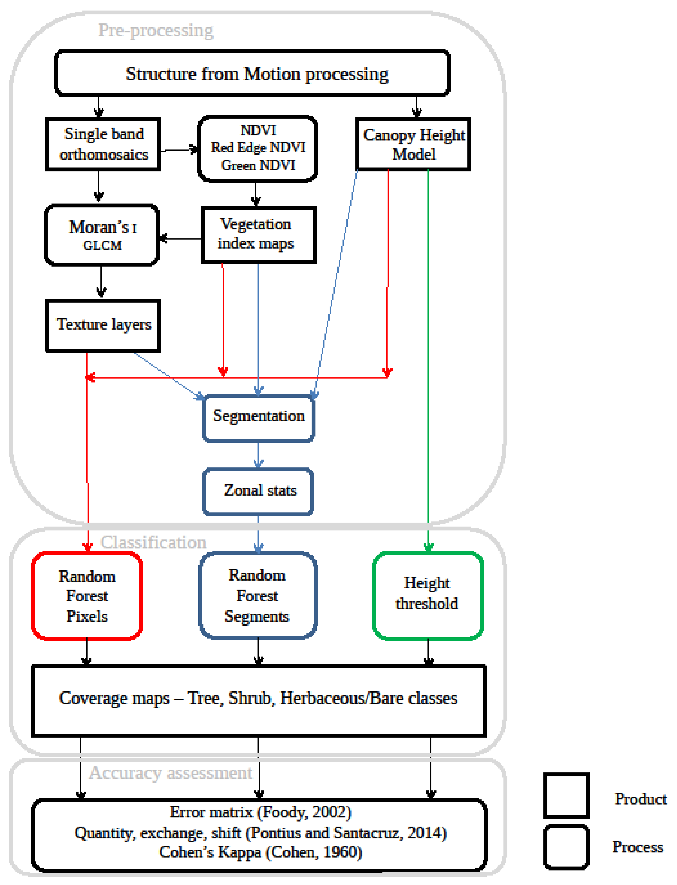
2.3. Data Processing Overview

Figure 2 provides an overview of the workflow. Initial work indicated that NIR CHMs showed the most agreement with in situ canopy height and radius measurements despite relatively coarse spatial resolutions [37], and they provided the baseline NIR-derived CHMs for each plot. We were unable to apply a radiometric calibration workflow due to oversaturation in calibration images taken in the field prior to each flight. Since we relied only on the within-image radiometric calibration applied by the Pix4D software made possible by the Sequoia sunlight irradiance sensor, we chose to rely exclusively on ratio-based optical indices rather than single-band reflectance maps with values that may vary greatly between flights. We extracted the individual normalized difference indices calculated using the green, red edge, and NIR bands in combination with the visible red band from the Parrot Sequoia sensor. These are common, easily calculable, and interpretable indices commonly used in vegetation studies.

(Gr, RE, or IR − Red)/(Gr, RE, or IR + Red).

(1)

For all spectral indices derived (Equation (1)), we calculated 3 × 3 pixel windows for contrast, dissimilarity, entropy, homogeneity, and second moment using the gray-level cooccurrence matrices (GLCM) package and local Moran’s I using the raster package in R (Vienna, Austria) v3.4.0 [44]. By using the GLCM package and outputs, we gathered textural properties throughout the image that could be useful for distinguishing between objects that may have had similar spectral reflectance values. We used local Moran’s I to find areas in the images that exhibited varying degrees of spatial autocorrelation, which could be useful for segmenting objects (woody individuals) we sought to classify. These metrics were shown to improve OBIA segmentation in urban areas [45], and they are useful for describing vegetation structure at coarser resolutions [46]. We then stacked all layers for each respective plot (CHM, ratio-based spectral indices, and textural properties) for segmentation.

2.4. Segmentation Units/Parameters

We iteratively tested a range of shape, compactness, and scale parameters to establish an appropriate segmentation approach [38]. Due to the relatively high resolution of UAS products, we selected a scale parameter of 10 to produce a reasonable aggregation of pixels, striking a balance between over- and under-segmentation [47] to capture tree and shrub crowns.

We segmented all UAS scenes using eCognition software (Definiens Developer v 9.5, Sunnyvale, CA, USA), with objects delineated on the basis of CHMs, ratio-based spectral indices, and textural properties. The band ratios helped alleviate potential radiometric inconsistencies between flights. Along with spectral properties, segmentation of objects into high-resolution imagery benefits from considering textural image properties [48,49].

Woody vegetation in our study area (predominantly Vachellia and Senegalia spp.) often exhibited highly irregular crowns; thus, we assigned a greater weight to layer values by assigning the shape parameter a value of 0.1. We equally weighted all rasters in the stack with a value of 1 except for CHM which we assigned a weight of 2 with the rationale that this layer directly represents the structural attributes of interest. Zonal statistics were calculated on the final segmentation layer for each site, and those metrics were then used as an input into the segment-based RF classifier.

2.5. Analytical Framework

For training and assessment of FVC estimates, 100 points were generated randomly within each site (n = 9) for a total of 900 reference points. Points were classified manually from the derived ~4 cm RGB orthomosaics as “tree”, “shrub”, or “other” (where other comprises grass and bare ground) according to visual identification, shadow depth, and expert site knowledge. Since our comparison measures of ultimate interest were areal estimates of proportional vegetation coverage at the plot level, compared across estimation processes, we used only the pixel-based unit of analysis for validation to estimate these plot-level measures. With the focus of distinguishing between woody vegetation types, “tree” points were meant to represent woody vegetation greater than 3 m in height, “shrub” points denoted woody vegetation from 1 to 3 m in height, and “other” comprised all vegetation less than 1 m in height, as well as bare ground. If points were on the edge of a given object, we manually moved these to ensure they were completely within an object of interest.

We then randomly sampled these reference points into points for training and those withheld for validation. Shrubs were made up the smallest number of expert-classified points (N = 147). We randomly assigned 70% of these (N = 102) for training and 30% of these to validation (N = 44). For both “tree” and “other” points, we then selected equal numbers of training (N = 102) and validation points (N = 44) from the larger number of total hand-classified points for a class-balanced set for both training and validation (306 training points and 132 validation points total). Class-balancing was used in order to not bias classification accuracy for more frequently occurring vegetation types.

We compared three different FVC techniques: a pixel-based random forest (P-RF), an object- or segmentation-based random forest (S-RF), and a thresholding approach, and we evaluated their mean relative difference from a hand classification of random points. The P-RF and S-RF leverage a nonparametric decision tree classifier [33], which provides a robust method to estimate FVC on the basis of a collection of remotely sensed input variables (Figure 1). As per Breiman’s original description of the random forest approach to classification and regression [36], a random forest is an ensemble approach, consisting of a collection of classifiers or trees, {h(x,Θ_k), k = 1, …}, where {Θ_k} denotes independent identically distributed vectors randomly sampled from the training data (bagging), and each tree casts a unit vote for the most popular class at input x. In addition, the forests use randomly selected inputs or combinations of inputs at each node to grow each classifier, h(x,Θ_k), which minimizes correlation between individual trees in the forest and confers additional robustness to overfitting and bias across the forest [48]. The RF algorithm allows for any number of continuous and discrete covariates to inform the classifier, which can be trained and used to estimate FVC at the pixel or object level. Individual observations not selected for any one individual tree can be used as independent or “out-of-bag” (OOB) estimates for RF model explanatory power, in addition to allowing simple variable importance estimates in conjunction with covariate resampling. Combined, these techniques result in classifiers that are highly accurate, robust to outliers and noise, faster than “boosting” techniques, and therefore, highly suitable for classification in remote sensing contexts [32].

Model estimation, fitting, and classification were conducted using the randomForest package in R [49], with automated tuning of the number of variables sampled for each split attained using the tuneRF function. For the P-RF model, the parameter settings used 500 trees, with five variables tried for each split in the forest. For the S-RF, the number of variables tried at each split was 20. These parameters were selected after automated tuning. The training data for the P-RF used covariate measures based on individual pixel values sampled at the points that were visually classified and randomly sampled (n = 28). The S-RF included the mean, standard deviation, maximum, and minimum values for each covariate layer’s pixels whose center fell inside the training object (n = 112). Lastly, as a comparison to the two RF modeling approaches, we also employed a threshold approach based on the UAS-derived canopy height model (CHM). All pixels with a CHM value greater than 3 m were classified as “tree”, those with a CHM value from 1 to 3 m were classified as “shrub”, and those with a CHM value below 1 m were classified as “other” following previous studies in the savanna context [37,50]. The 3 m threshold was used in the field to objectively separate woody biomass into tree or shrub categories.

2.6. Technique Agreement Measures

To determine whether there are meaningful differences between classification methods, we calculated a series of standard classification metrics using the withheld validation points. Because these were aggregated across all nine sites, we present metrics unweighted by class representation, which would otherwise be preferred [51]. Weighted values would result in different outputs due to changing site-to-site composition of tree/shrub/other in each site as a whole. Since our points are representative across all sites, the unweighted values provide a means to compare classification techniques but not assess site-level accuracies.

The calculated agreement measures include error matrices (also known as contingency tables or confusion matrices) [52], Cohen’s kappa index [53], omission, commission, and agreement measures [54], and a set of metrics known as quantity, exchange, and shift [51].

Table 1. Technique comparison agreement measures.

Type	Description	References
Error matrix	Cross tabulation of n × n array of land-cover classes. Columns represent the reference data; rows denote mapped land-cover class.	[51]
Omission	Number of reference points left out from the intended mapped land-cover class.	[54]
Commission	Number of reference points for a given class incorrectly mapped to a different land-cover class in the land-cover output.	[54]
Agreement	Total number of correctly classified reference points in the final mapped output.	[54]
Quantity	Amount of absolute difference between the reference map and a comparison map due to the less than perfect match in the proportions of the categories.	[51]
Exchange	Exchange occurs as a one-to-one difference between two categories. These differences do not reflect the quantity differences of the classes, but rather a spatial mismatch.	[51]
Shift	Shift represents the leftover disagreement after subtracting quantity and exchange differences from the total. These differences are due to exchanges occurring among >2 map classes.	[51]
Cohen’s kappa (unweighted)	Measure of agreement between a land-cover map and a set of reference points, corrected for chance uncertainty.	[53]

provides a definition and rationale for the chosen metrics.

Lastly, to quantitatively compare classification approaches across vegetation structural conditions, within the context of estimating FVC, we estimated FVCs at the site level using four approaches. The first approach uses the by-hand classification of randomly selected points and the remaining three approaches use the classified, rasterized estimates from the UAS-derived, multispectral imagery for each of the nine study area sites. Site selection was stratified by dominant vegetation condition, with three of each grass-, shrub-, and tree-dominated condition chosen.

3. Results

3.1. Random Forest Models

The P-RF classification model had an OOB classification error rate of 21.24%. OOB errors are calculated using a random sample of reference observations that are withheld for each tree in the random forest. These are then classified for each tree, and the error rate is then calculated across all trees in the random forest. In Figure 3a, the most important covariate informing the P-RF classification is the CHM, as indicated by the mean decrease in Gini metric. The mean decrease in Gini captures the average of a variable’s total decrease in node impurity, a metric of per-class sorting, weighted by the proportion of training samples that reach a particular node in each individual decision tree, and then averaged across all trees in the random forest. For the P-RF, the CHM covariate was followed by red-edge NDVI covariates and then the NIR-based NDVI metrics.

For the S-RF classification model, zonal statistics (mean, maximum, minimum, and standard deviation) of each covariate were calculated from the rasterized covariate pixels within each segmented polygon. Polygons containing a training point were assigned to that point’s class and used as reference and holdout data for the RF. The OOB error for the S-RF was lower than the P-RF at 13.4%. Similar to the P-RF, variable importance metrics indicate that the CHM variables were the most important covariates for classifying land components (Figure 3b). However, in the segment-based RF model, the additional CHM-derived segment metrics (i.e., maximum canopy height and the standard deviation of canopy height) were ranked higher than individual band metrics (e.g., red-edge NDVI), although red-edge metrics made it into the top five.

3.2. Classification Approach—Accuracy Assessment

Figure 4 is a visualization from a representative of each site type (tree-, shrub-, and grass-dominated), which illustrates qualitative differences between the classification approaches. FVC estimates from each approach will naturally vary, as shown overlaid with the hand-classified points and accompanied by high-resolution imagery. Each panel in Figure 4 gives the Mavic-derived orthomosaic for the full flight extent and a zoomed-in portion of the site to highlight the overlay of visually inspected points relative to FVC-estimated land cover. The FVC surfaces are shown for each classification approach. The S-RF includes the segmented polygons overlayed in gray. Notably, for the S-RF FVC output, since it is “object-based,” the classified vegetation is more contiguous than the pixel-based approach as entire polygons are classified as a single vegetation type. These are contrasted with the simpler CHM threshold approach and its three height classes. Qualitatively, the threshold approach also produces relatively more contiguous areas than the P-RF classification.

Table 2. Classification assessment output for (a) P-RF, (b) S-RF, and (c) threshold techniques for quantifying fractional vegetation coverage.

(a) Pixel-Based RF (P-RF)
Error Matrix Unweighted
	Other	Shrub	Tree
Other	42	6	0
Shrub	2	35	5
Tree	0	3	39
Kappa Unweighted
	Value	ASE	z	Pr(>|z|)
	0.8182	0.04253	19.24	1.79E-82
Difference Table
	Category	Omission	Agreement	Commission	Quantity	Exchange	Shift
1	Other	2	42	6	4	4	0
2	Shrub	9	35	7	2	10	4
3	Tree	5	39	3	2	6	0
4	Overall	16	116	16	4	10	2
(b) Segment-Based RF (S-RF)
Error Matrix Unweighted
	Other	Shrub	Tree
Other	36	3	2
Shrub	8	37	10
Tree	0	4	32
Kappa Unweighted
	Value	ASE	z	Pr(>|z|)
	0.6932	0.05247	13.21	7.69E-40
Difference Table
	Category	Omission	Agreement	Commission	Quantity	Exchange	Shift
1	Other	8	36	5	3	6	4
2	Shrub	7	37	18	11	14	0
3	Tree	12	32	4	8	8	0
4	Overall	27	105	27	11	14	2
(c) Canopy Height Threshold
Error Matrix Unweighted
	Other	Shrub	Tree
Other	43	15	0
Shrub	1	27	6
Tree	0	2	38
Kappa Unweighted
	Value	ASE	z	Pr(>|z|)
	0.7273	0.04947	14.7	6.30E-49
Difference Table
	Category	Omission	Agreement	Commission	Quantity	Exchange	Shift
1	Other	1	43	15	14	2	0
2	Shrub	17	27	7	10	6	8
3	Tree	6	38	2	4	4	0
4	Overall	24	108	24	14	6	4

quantitatively compares the classification results across the class-balanced set of held-out reference points for each classification approach (the complete, unbalanced validation data are presented in Table S1). The quantitative metrics outlined in the methods show that, at the reference point level, the P-RF has the highest overall agreement. Examining only the error matrix for each classifier, “tree” and “shrub” points were more likely to be misclassified than the “other” class. The quantity metric showed the most change in the CHM threshold approach between the classified map and reference points. This directly relates to the exchange, or confusion, between “shrub” and “other” borne out in the error matrix. The RF-based classification showed higher quantity disagreement with the segment-based approach than the pixel-based approach, but both RF-models showed more confusion in the exchange and shift metrics when compared to the CHM threshold approach.

3.3. Site Type Characterization

We present these site-level FVC estimates separated by vegetation type (each panel) and broken down by dominant site type (x-axis category) and image classification approach (symbol) in Figure 5.

These results show that, at the site level, estimates of FVC do vary between classification approaches. The widest range of disagreement between classification approaches occurred for shrub and other coverage estimates. These variations, as indicated in Table 2, were driven primarily by differences in the classification accuracy for shrubs across all sites and were particularly high in shrub-dominated sites. To further refine these differences between the classified output and the by-hand approach, Figure 6 shows the mean relative difference in fractional vegetation cover, estimated by each classified and rasterized approach, from which the FVC estimated from the random sample of reference points within each study site was subtracted. These differences were aggregated across all sites and site types, yielding a point estimate (N = 9) and a 95% confidence interval. This yielded statistically significant differences at the α = 0.05 level between any one classification approach and the by-hand estimates in FVC when the CI did not overlap zero.

These results suggest that the pixel-based classification approach (P-RF) has the highest level of agreement with FVC estimated by hand classification of random points, across all site structural types. The CHM threshold approach tended to overestimate the amount of “other” vegetation cover, and the S-RF approach tended to overestimate the amount of “shrub” vegetation.

4. Discussion

In this study, we provided an illustration of classification techniques and remotely sensed approaches for mapping FVC using UAS imagery. We build on the use of the UAS NIR band in delineating structural and compositional landscape features [36] to demonstrate the value of structural vegetation information in the infrared spectral range in classifying savanna landscape function. We also emphasize, through our set of classification comparisons, the importance of integrating remote sensing methods and underlying statistical considerations for mapping FVC and structural conditions.

With respect to whether estimates of FVC vary with classification strategy, our findings denote statistically significant differences in the agreement of the classification methods (Table 2), with the most disagreement between approaches occurring for shrub-dominated sites (Figure 5). Additionally, the P-RF method had the highest overall agreement across classification techniques and was the only approach not to differ significantly from a hand-delineated FVC estimation.

Image acquisition times concurred with onset of the dry season, when “greenness” signatures corresponded to the “tree” and “shrub” components, with the senesced grass cover combined with bare soil and non-photosynthesizing components for the “other” class. Using the NIR output from the UAS point cloud processing, we were able to leverage both spectral and structural properties of different vegetation landscape features [55]. Interestingly, while the high spatial fidelity of the UAS lends itself toward OBIA techniques for differentiating individual species on the landscape [56,57], the P-RF classifier had higher agreement across classes than the S-RF classifier. This may relate to the additional covariates included in the S-RF and a subsequent smoothing effect due to segments and their aggregated, averaged characteristics (not single pixels) informing the final FVC output (Figure 4). Overlaid with the validation points, that smoothing effect may have masked actual variability in landscape features better captured by the P-RF and CHM threshold approaches. In addition, the validation polygons for the S-RF model were assigned the same class as that of a hand-delineation point located within the polygon. We assumed that the polygon represents a within-unit homogeneity that may include some level of error due to either (a) the accuracy in the segmentation process or (b) the “truth” in the hand-delineated class assignments. We recognize the inherent error and bias in the hand-delineation approach to identifying reference validation points used in the accuracy assessment of classification approaches. However, in situ ground reference will have its own bias and error. CHM variables were the most important covariates for classifying across FVC land classes.

The CHM variables were the most important covariates in both RF classifications (Figure 3), as also shown in other studies [58]. There is a reasonable argument that VHR imagery and visual assessment of landscape features can be used for training a straightforward CHM threshold classifier to estimate FVC across a landscape. While, in this study, the CHM threshold classifier did not have the highest overall agreement in the balanced class case, it performed better than the S-RF classifier and more accurately distinguished between “shrub” and “tree” classes than either RF classifier. This clearly may relate to the physical criteria established during field work for delineating trees from other woody biomass, centered on 3 m exceedance. The ability to hand-delineate points falling on trees vs. shrubs in high-resolution imagery also relies on contextual clues such as shadow and configuration that directly relate to vegetation height. Thus, a CHM-based classifier alone, even one based simply on threshold setting, might be useful. Such an approach reduces the model and classification parameterization choices, processing time, and data aggregation that a machine-learning approach would require [27].

The most challenging and widely varying disagreement in the FVC estimates was shrub cover. All three classifiers struggled to accurately capture the shrub FVC as estimated from the by-hand point classification. While the P-RF based classification method was the most robust classification method overall, if the focus of analysis was based on separating out woody biomass components on a landscape, the CHM threshold approach more accurately distinguished between tree and shrubs than either RF-based approach. This underscores the utility of remotely sensed data, which results in the ability to distinguish some aspects of vegetation structure in this type of classification context (e.g., LIDAR, UAS-derived point clouds, etc.).

Lastly, we suggest further research regarding ensemble-based, machine-learning approaches and the application of reference point selection. Prior research has shown that classification algorithms may be sensitive to unbalanced training data, with respect to the number of representative observations from each class [59]. While RF-based approaches which use a combination of covariate randomization and bagging across an ensemble of model classifiers minimize certain biases [33,49], our results indicate that class imbalance in training data may be yielding a disconnect between classification accuracy as measured by OOB error at the model level and the error as measured against a balanced, withheld set of reference data. We chose to focus the analysis of classifier accuracy on each of three classes by using the balanced data, at a site level, from which we are interested in estimating FVC. However, it may be more important to classify the relative amounts of vegetation more accurately. We present unbalanced, withheld error matrices as supplemental information (Table S1) for comparison and further consideration, but suggest that more research be conducted on site, sub-site, and pixel-level classification for FVC estimates that directly explore the impact of balanced vs. unbalanced training and reference data. In addition, other types of classification optimization could be undertaken (e.g., [60]), which might further refine the ability to yield site-level FVC estimates. This may be especially important as it relates to the relative contribution to classification accuracy of structural vs. spectral data to the classifier, especially in different contexts where the relative value of “greenness” versus vegetation height might have different value (e.g., when using imagery collected during the rainy season or in more vegetated contexts).

5. Conclusions

Differences in the structural aspects of tree and shrub proportions provide valuable insight into the land function for habitat health, livelihood resources, and ecosystem connectedness [13,14]. This study emphasized two important points: (1) the importance of critical decision points in data processing which in turn should be driven by the type of problem or question being addressed [59]; (2) identification of a set of considerations that need to be carefully weighed when selecting a remote sensing approach and classification technique for landscapes where variation in landscape composition or structural attributes impact land function. The spectral information on “greenness” combined with canopy structure information provides an indication of current resource availability and ecological function of savanna range conditions [61]. The addition of canopy structure information is notable for savanna environments where landscape-level degradation of ecosystem functioning over the long term has important implications for wildlife and livestock [50], and which may not be detectable through “greenness” alone, e.g., in the case of shrub encroachment. Indeed, canopy structure is arguably the most important variable to inform savanna FVC, as noted in the variable importance plots (Figure 3) and the comparable accuracy of the CHM threshold model (Table 2). Identifying the “best” method to extract the remotely sensed ecological information does not have one right or wrong answer, but decision points for tradeoffs in different classification methods, sensitivity tests, acceptable error rates, unit of analysis, etc. will all depend on the research or management objective. Through careful reflection on these different points of analysis, remotely sensed landscape analyses will translate into relevant and timely information beyond the “greenness” factor in semiarid landscapes that support large populations of both people and wildlife.

References

1. Cherlet, M.; Hutchinson, C.; Reynolds, J.; Hill, J.; Sommer, S.; von Maltitz, G. World Atlas of Desertification: Rethinking Land Degradation and Sustainable Land Management; Publications Office of the European Commission: Luxenbourg, 2018. [Google Scholar]
2. Feng, S.; Fu, Q. Expansion of global drylands under a warming climate. Atmos. Chem. Phys. 2013, 13, 10081–10094. [Google Scholar] [CrossRef] [Green Version]
3. Holdridge, L.R. Determination of world plant formations from simple climatic data. Science 1947, 105, 367–368. [Google Scholar] [CrossRef]
4. Touboul, J.D.; Staver, A.C.; Levin, S.A. On the complex dynamics of savanna landscapes. Proc. Natl. Acad. Sci. USA 2018, 115, E1336–E1345. [Google Scholar] [CrossRef] [Green Version]
5. Archer, S.R.; Andersen, E.M.; Predick, K.I.; Schwinning, S.; Steidl, R.J.; Woods, S.R. Woody plant encroachment: Causes and consequences. In Rangeland Systems: Processes, Management and Challenges; Briske, D.D., Ed.; Springer Series on Environmental Management; Springer International Publishing: Cham, Germany, 2017; pp. 25–84. ISBN 978-3-319-46709-2. [Google Scholar]
6. Liu, J.; Dietz, T.; Carpenter, S.R.; Alberti, M.; Folke, C.; Moran, E.; Pell, A.N.; Deadman, P.; Kratz, T.; Lubchenco, J.; et al. Complexity of coupled human and natural systems. Science 2007, 317, 1513–1516. [Google Scholar] [CrossRef] [Green Version]
7. Sala, O.E.; Maestre, F.T. Grass–woodland transitions: Determinants and consequences for ecosystem functioning and provisioning of services. J. Ecol. 2014, 102, 1357–1362. [Google Scholar] [CrossRef]
8. Gamon, J.A.; Qiu, H.-L.; Sanchez-Azofeifa, A. Ecological applications of remote sensing at multiple scales. In Functional Plant Ecology; CRC Press: Boca Raton, FL, USA, 2007; ISBN 978-0-429-12247-7. [Google Scholar]
9. Whiteside, T.G.; Boggs, G.S.; Maier, S.W. Comparing object-based and pixel-based classifications for mapping savannas. Int. J. Appl. Earth Obs. Geoinf. 2011, 13, 884–893. [Google Scholar] [CrossRef]
10. Mishra, N.B.; Crews, K.A.; Okin, G.S. Relating spatial patterns of fractional land cover to savanna vegetation morphology using multi-scale remote sensing in the central kalahari. Int. J. Remote Sens. 2014, 35, 2082–2104. [Google Scholar] [CrossRef] [Green Version]
11. Belgiu, M.; Drăguţ, L. Random forest in remote sensing: A review of applications and future directions. ISPRS J. Photogramm. Remote Sens. 2016, 114, 24–31. [Google Scholar] [CrossRef]
12. Brandt, M.; Tucker, C.J.; Kariryaa, A.; Rasmussen, K.; Abel, C.; Small, J.; Chave, J.; Rasmussen, L.V.; Hiernaux, P.; Diouf, A.A.; et al. An unexpectedly large count of trees in the West African Sahara and Sahel. Nature 2020, 587, 78–82. [Google Scholar] [CrossRef]
13. Riva, F.; Nielsen, S.E. A Functional perspective on the analysis of land use and land cover data in ecology. Ambio 2021, 50, 1089–1100. [Google Scholar] [CrossRef]
14. Venter, Z.S.; Cramer, M.D.; Hawkins, H.-J. Drivers of woody plant encroachment over Africa. Nat. Commun. 2018, 9, 2272. [Google Scholar] [CrossRef] [Green Version]
15. Asner, G.; Levick, S.; Smit, I. Remote sensing of fractional cover and biochemistry in savannas. In Ecosystem Function in Savannas; Hill, M.J., Hanan, N.P., Eds.; CRC Press: Boca Raton, FL, USA, 2010; pp. 195–218. ISBN 978-1-4398-0470-4. [Google Scholar]
16. Chadwick, K.D.; Asner, G.P. Organismic-scale remote sensing of canopy foliar traits in lowland tropical forests. Remote Sens. 2016, 8, 87. [Google Scholar] [CrossRef] [Green Version]
17. Staver, A.C.; Archibald, S.; Levin, S. Tree cover in Sub-Saharan Africa: Rainfall and fire constrain forest and savanna as alternative stable states. Ecology 2011, 92, 1063–1072. [Google Scholar] [CrossRef]
18. Scholes, R.J.; Dowty, P.R.; Caylor, K.; Parsons, D.A.B.; Frost, P.G.H.; Shugart, H.H. Trends in savanna structure and composition along an aridity gradient in the Kalahari. J. Veg. Sci. 2002, 13, 419–428. [Google Scholar] [CrossRef]
19. Chadwick, K.D.; Brodrick, P.G.; Grant, K.; Goulden, T.; Henderson, A.; Falco, N.; Wainwright, H.; Williams, K.H.; Bill, M.; Breckheimer, I.; et al. Integrating airborne remote sensing and field campaigns for ecology and earth system science. Methods Ecol. Evol. 2020, 11, 1492–1508. [Google Scholar] [CrossRef]
20. Munyati, C.; Economon, E.B.; Malahlela, O.E. Effect of canopy cover and canopy background variables on spectral profiles of savanna rangeland bush encroachment species based on selected acacia species (Mellifera, Tortilis, Karroo) and Dichrostachys Cinerea at Mokopane, South Africa. J. Arid Environ. 2013, 94, 121–126. [Google Scholar] [CrossRef]
21. Anderson, K.; Gaston, K. Lightweight unoccupied aerial vehicles will revolutionize spatial ecology. Front. Ecol. Environ. 2013, 11, 138–146. [Google Scholar] [CrossRef] [Green Version]
22. Hardin, P.J.; Lulla, V.; Jensen, R.R.; Jensen, J.R. Small unoccupied aerial systems (SUAS) for environmental remote sensing: Challenges and opportunities revisited. GISci. Remote Sens. 2019, 56, 309–322. [Google Scholar] [CrossRef]
23. Melville, B.; Lucieer, A.; Aryal, J. Classification of lowland native grassland communities using hyperspectral unoccupied aircraft system (UAS) imagery in the tasmanian midlands. Drones 2019, 3, 5. [Google Scholar] [CrossRef] [Green Version]
24. Räsänen, A.; Virtanen, T. Data and resolution requirements in mapping vegetation in spatially heterogeneous landscapes. Remote Sens. Environ. 2019, 230, 111207. [Google Scholar] [CrossRef]
25. Smith, M.W.; Carrivick, J.L.; Quincey, D.J. Structure from motion photogrammetry in physical geography. Prog. Phys. Geogr. Earth Environ. 2016, 40, 247–275. [Google Scholar] [CrossRef] [Green Version]
26. Kedia, A.C.; Kapos, B.; Liao, S.; Draper, J.; Eddinger, J.; Updike, C.; Frazier, A.E. An integrated spectral–structural workflow for invasive vegetation mapping in an arid region using drones. Drones 2021, 5, 19. [Google Scholar] [CrossRef]
27. Gränzig, T.; Fassnacht, F.E.; Kleinschmit, B.; Förster, M. Mapping the fractional coverage of the invasive Shrub Ulex Europaeus with multi-temporal sentinel-2 imagery utilizing UAV orthoimages and a new spatial optimization approach. Int. J. Appl. Earth Obs. Geoinf. 2021, 96, 102281. [Google Scholar] [CrossRef]
28. Xu, Z.; Shen, X.; Cao, L.; Coops, N.C.; Goodbody, T.R.H.; Zhong, T.; Zhao, W.; Sun, Q.; Ba, S.; Zhang, Z.; et al. Tree species classification using UAS-based digital aerial photogrammetry point clouds and multispectral imageries in subtropical natural forests. Int. J. Appl. Earth Obs. Geoinf. 2020, 92, 102173. [Google Scholar] [CrossRef]
29. Stehman, S.V.; Wickham, J.D. Pixels, blocks of pixels, and polygons: Choosing a spatial unit for thematic accuracy assessment. Remote Sens. Environ. 2011, 115, 3044–3055. [Google Scholar] [CrossRef]
30. Ye, S.; Pontius, R.G.; Rakshit, R. A review of accuracy assessment for object-based image analysis: From per-pixel to per-polygon approaches. ISPRS J. Photogramm. Remote Sens. 2018, 141, 137–147. [Google Scholar] [CrossRef]
31. Bruzzone, L.; Demir, B. A review of modern approaches to classification of remote sensing data. In Land Use and Land Cover Mapping in Europe: Practices & Trends; Manakos, I., Braun, M., Eds.; Remote Sensing and Digital Image Processing; Springer: Dordrecht, The Netherlands, 2014; pp. 127–143. ISBN 978-94-007-7969-3. [Google Scholar]
32. Maxwell, A.E.; Warner, T.A.; Fang, F. Implementation of machine-learning classification in remote sensing: An applied review. Int. J. Remote Sens. 2018, 39, 2784–2817. [Google Scholar] [CrossRef] [Green Version]
33. Breiman, L. Random forests. Mach. Learn. 2001, 45, 5–32. [Google Scholar] [CrossRef] [Green Version]
34. Jawak, S.D.; Devliyal, P.; Luis, A.J. A Comprehensive review on pixel oriented and object oriented methods for information extraction from remotely sensed satellite images with a special emphasis on cryospheric applications. Adv. Remote Sens. 2015, 4, 177–195. [Google Scholar] [CrossRef] [Green Version]
35. Chenari, A.; Erfanifard, Y.; Dehghani, M.; Pourghasemi, H.R. Woodland mapping and single-tree levels using object-oriented classification of unoccupied aerial vehicle (UAV) images. ISPRS Int. Arch. Photogramm. Remote Sens. Spat. Inf. Sci. 2017, 42, 43–49. [Google Scholar] [CrossRef] [Green Version]
36. Blaschke, T. Object based image analysis for remote sensing. ISPRS J. Photogramm. Remote Sens. 2010, 65, 2–16. [Google Scholar] [CrossRef] [Green Version]
37. Kolarik, N.E.; Gaughan, A.E.; Stevens, F.R.; Pricope, N.G.; Woodward, K.; Cassidy, L.; Salerno, J.; Hartter, J. A multi-plot assessment of vegetation structure using a micro-unoccupied aerial system (UAS) in a semi-arid savanna environment. ISPRS J. Photogramm. Remote Sens. 2020, 164, 84–96. [Google Scholar] [CrossRef] [Green Version]
38. Salerno, J.; Cassidy, L.; Drake, M.; Hartter, J. Living in an Elephant Landscape: The local communities most affected by wildlife conservation often have little say in how it is carried out, even when policy incentives are intended to encourage their support. Am. Sci. 2018, 106, 34–41. [Google Scholar]
39. Gaughan, A.; Waylen, P. Spatial and temporal precipitation variability in the Okavango-Kwando-Zambezi catchment, Southern Africa. J. Arid Environ. 2012, 82, 19–30. [Google Scholar] [CrossRef]
40. Pricope, N.G.; Gaughan, A.E.; All, J.D.; Binford, M.W.; Rutina, L.P. Spatio-temporal analysis of vegetation dynamics in relation to shifting inundation and fire regimes: Disentangling environmental variability from land management decisions in a Southern African transboundary watershed. Land 2015, 4, 627–655. [Google Scholar] [CrossRef]
41. Elliott, K.C.; Montgomery, R.; Resnik, D.B.; Goodwin, R.; Mudumba, T.; Booth, J.; Whyte, K. Drone use for environmental research [Perspectives]. IEEE Geosci. Remote Sens. Mag. 2019, 7, 106–111. [Google Scholar] [CrossRef]
42. Pix4D Pix4Dmapper 4.1 USER MANUAL. Available online: https://support.pix4d.com/hc/en-us/articles/204272989-Offline-Getting-Started-and-Manual-pdf (accessed on 7 July 2021).
43. Pricope, N.G.; Mapes, K.L.; Woodward, K.D.; Olsen, S.F.; Baxley, J.B. Multi-sensor assessment of the effects of varying processing parameters on UAS product accuracy and quality. Drones 2019, 3, 63. [Google Scholar] [CrossRef] [Green Version]
44. R Core Team. R: A Language and Envrionment for Statistical Computing; R Foundation for Statistical Computing: Vienna, Austria, 2020. [Google Scholar]
45. Su, W.; Li, J.; Chen, Y.; Liu, Z.; Zhang, J.; Low, T.M.; Suppiah, I.; Hashim, S.A.M. Textural and local spatial statistics for the object-oriented classification of urban areas using high resolution imagery. Int. J. Remote Sens. 2008, 29, 3105–3117. [Google Scholar] [CrossRef]
46. Farwell, L.S.; Gudex-Cross, D.; Anise, I.E.; Bosch, M.J.; Olah, A.M.; Radeloff, V.C.; Razenkova, E.; Rogova, N.; Silveira, E.M.O.; Smith, M.M.; et al. Satellite image texture captures vegetation heterogeneity and explains patterns of bird richness. Remote Sens. Environ. 2021, 253, 112175. [Google Scholar] [CrossRef]
47. Liu, D.; Xia, F. Assessing object-based classification: Advantages and limitations. Remote Sens. Lett. 2010, 1, 187–194. [Google Scholar] [CrossRef]
48. Breiman, L. Bagging predictors. Mach. Learn. 1996, 24, 123–140. [Google Scholar] [CrossRef] [Green Version]
49. Liaw, A.; Wiener, M. Classification and regression by randomForest. R News 2002, 2, 5. [Google Scholar]
50. Fisher, J.T. Savanna woody vegetation classification—Now in 3-D. Appl. Veg. Sci. 2014, 17, 172–184. [Google Scholar] [CrossRef]
51. Pontius, R.; Santacruz, A. Quantity, exchange, and shift components of difference in a square contingency table. Int. J. Remote Sens. 2014, 35, 7543–7554. [Google Scholar] [CrossRef]
52. Foody, G.M. Status of land cover classification accuracy assessment. Remote Sens. Environ. 2002, 80, 185–201. [Google Scholar] [CrossRef]
53. Cohen, J. A Coefficient of agreement for nominal scales. Educ. Psychol. Meas. 1960, 20, 37–46. [Google Scholar] [CrossRef]
54. Story, M.; Congalton, R.C. Accuracy assessment: A user’s perspective. Photogramm. Eng. Remote Sens. 1986, 52, 397–399. [Google Scholar]
55. Smith, W.K.; Dannenberg, M.P.; Yan, D.; Herrmann, S.; Barnes, M.L.; Barron-Gafford, G.A.; Biederman, J.A.; Ferrenberg, S.; Fox, A.M.; Hudson, A.; et al. Remote sensing of dryland ecosystem structure and function: Progress, challenges, and opportunities. Remote Sens. Environ. 2019, 233, 111401. [Google Scholar] [CrossRef]
56. Lu, B.; He, Y. Species classification using unoccupied aerial vehicle (UAV)-acquired high spatial resolution imagery in a heterogeneous grassland. ISPRS J. Photogramm. Remote Sens. 2017, 128, 73–85. [Google Scholar] [CrossRef]
57. Melville, B.; Fisher, A.; Lucieer, A. Ultra-high spatial resolution fractional vegetation cover from unoccupied aerial multispectral imagery. Int. J. Appl. Earth Obs. Geoinf. 2019, 78, 14–24. [Google Scholar] [CrossRef]
58. Pádua, L.; Guimarães, N.; Adão, T.; Marques, P.; Peres, E.; Sousa, A.; Sousa, J.J. Classification of an agrosilvopastoral system using RGB imagery from an unoccupied aerial vehicle. In Progress in Artificial Intelligence; Moura Oliveira, P., Novais, P., Reis, L.P., Eds.; Lecture Notes in Computer Science; Springer International Publishing: Cham, Switzerland, 2019; Volume 11804, pp. 248–257. ISBN 978-3-030-30240-5. [Google Scholar]
59. Weiss, G.M.; Provost, F. The effect of class distribution on classifier learning. In Technical Report ML-TR-43; Department of Computer Science, Rutgers University, 2001; Available online: https://storm.cis.fordham.edu/~gweiss/papers/ml-tr-44.pdf (accessed on 22 December 2021). [CrossRef]
60. Baldi, P.; Brunak, S.; Chauvin, Y.; Andersen, C.A.F.; Nielsen, H. Assessing the accuracy of prediction algorithms for classification: An overview. Bioinformatics 2000, 16, 412–424. [Google Scholar] [CrossRef] [PubMed] [Green Version]
61. Scholtz, R.; Kiker, G.A.; Smit, I.P.J.; Venter, F.J. Identifying drivers that influence the spatial distribution of woody vegetation in Kruger National Park, South Africa. Ecosphere 2014, 5, 1–12. [Google Scholar] [CrossRef]
Figure 1. Individual sites (N = 9) for UAS flights in the study area. RGB composites shown for the Sequoia sensor (red = NIR, green = visible green, blue = red edge) for (Row A) grass-, (Row B) shrub-, and (Row C) tree-dominated landscapes in the Chobe Enclave of northern Botswana.
Remotesensing 14 00551 g001
Figure 2. Process flow outlining data input, UAS-extracted metrics for segmentation, and the three different methods for classification: height threshold (green), RF pixel (orange), and RF segments (blue).
Remotesensing 14 00551 g002
Figure 3. Variable importance for (a) pixel- and (b) segmented object-based RF models. Numbers represent the decrease in sorting efficiency measured by the Gini index when each variable is individually reshuffled and classes are re-predicted (we present all 28 covariates for P-RF, but the top 28 of 112 covariates for S-RF). Structural variables from the CHM are noted in orange.
Remotesensing 14 00551 g003
Figure 4. Classified maps for site types (a) woody, (b) shrub, and (c) other. Segments are overlaid on the predicted S-RF output. Black crosses represent visual inspection points that fall within each site area. The site area imagery and the inset (~4 cm nominal ground resolution) are also displayed for each using the Mavic orthomosaics.
Remotesensing 14 00551 g004aRemotesensing 14 00551 g004b
Figure 5. Classification approaches are compared by plotting the site-level FVC estimates from the entire classified image alongside visually hand-classified random points. Vegetation percentages of (a) trees, (b) shrubs, and (c) other by panel, by dominant vegetation site type (columns within each panel), separated by classification technique (color).
Remotesensing 14 00551 g005
Figure 6. Mean relative difference in FVC classification technique as compared to the expert, image-based delineation of reference points. Confidence intervals (95%) that do not cross the dotted line indicate a statistically significant difference for each FVC estimate for a given classification approach and the by-hand estimation.
Remotesensing 14 00551 g006