Abstract
In our current global warming climate, the growth of record-breaking heat waves (HWs) is expected to increase in its frequency and intensity. Consequently, the considerably growing and agglomerated world’s urban population becomes more exposed to serious heat-related health risks. In this context, the study of Surface Urban Heat Island (SUHI) intensity during HWs is of substantial importance due to the potential vulnerability urbanized areas might have to HWs in comparison to their surrounding rural areas. This article discusses Land Surface Temperatures (LST) reached during the extreme HW over Western North America during the boreal summer of 2021 using Thermal InfraRed (TIR) imagery acquired from TIR Sensor (TIRS) (30 m spatial resolution) onboard Landsat-8 platform and Moderate Resolution Imaging Spectroradiometer (MODIS) (1 km spatial resolution) onboard Terra/Aqua platforms. We provide an early assessment of maximum LSTs reached over the affected areas, as well as impacts in terms of SUHI over the main cities and towns. MODIS series of LST from 2000 to 2021 over urbanized areas presented the highest recorded LST values in late June 2021, with maximum values around 50 °C for some cities. High spatial resolution LSTs (Landsat-8) were used to map SUHI intensity as well as to assess the impact of SUHI on thermal comfort conditions at intraurban space by means of a thermal environmental quality indicator, the Urban Field Thermal Variance Index (UFTVI). The same high resolution LSTs were used to verify the existence of clusters and employ a Local Indicator of Spatial Association (LISA) to quantify its degree of strength. We identified the spatial distribution of heat patterns within the intraurban space as well as described its behavior across the thermal landscape by fitting a polynomial regression model. We also qualitatively analyze the relationship between both UFTVI and LST clusters with different land cover types. Findings indicate that average daytime SUHI intensity for the studied cities was typically within 1 to 5 °C, with some exceptional values surpassing 7 °C and 9 °C. During night, the SUHI intensity was reduced to variations within 1–3 °C, with a maximum value of +4 °C. The extreme LSTs recorded indicate no significant influence of HW on SUHI intensity. SUHI intensity maps of the intraurban space evidence hotspots of much higher values located at densely built-up areas, while urban green spaces and dense vegetation show lower values. In the same manner, UTFVI has shown “no” SUHI for densely vegetated regions, water bodies, and low-dense built-up areas with intertwined dense vegetation, while the “strongest” SUHI was observed for non-vegetated dense built-up areas with low albedo material such as concrete and pavement. LST was evidenced as a good marker for assessing the influence of HWs on SUHI and recognizing potential thermal environmental consequences of SUHI intensity. This finding highlights that remote-sensing based LST is particularly suitable as an indicator in the analysis of SUHI intensity patterns during HWs at different spatial resolutions. LST used as an indicator for analyzing and detecting extreme temperature events and its consequences seems to be a promising means for rapid and accurate monitoring and mapping.
1. Introduction
Heat waves (HWs) such as extreme weather events can be broadly defined upon the bases of an unusual heat stress forecast occurring for a continuous period of a minimum of 48 h to even weeks during which daytime high and nighttime low temperatures tend exceed a threshold with quasi-stationary anticyclone conditions. Such climatic events are known to cause temporary adverse consequences for human life and natural systems [1]. Nonetheless, specific definitions of such thresholds might be required for considering cases of different climate zones as well as population adaption capabilities. HWs are atmosphere–land surface related phenomena with impact in levels of soil moisture since they influence the energy fluxes between the atmosphere and the ground, directly impacting heat transfer processes and surface energy balances. Research in the Southcentral U.S. has shown that high HWs frequency results in sensible heat increase and latent heat fluxes decrease. It also indicated that HW intensity—which has impacts on surface heat and moisture—should be linked to the bio-geophysical properties of surfaces, suggesting positive land–atmosphere feedback of HWs [2].
The consequences of HWs could have devastating impacts for society and ecosystem functioning. HWs are considered one of the major causes of weather-related deaths [3], a major factor of human climate-sensitive disease [4], a reason of severe economic loss [5,6], a cause of environmental impact such as threatening sea-ice melting in the artic regions [7], vegetation degradation [8], droughts in soil moisture [9,10], and forests wildfires [11], as well as its negative effects on biodiversity [12] and species richness [13] together with severe consequences in marine ecosystems [14]. Recently globally growing record-breaking HWs have been associated with the consequences of global warming produced by human influence on climate, while predictions indicate that these phenomena will tend to increase in a warming climate, expanding its frequency and intensity [15,16]. Empirical studies in China based upon air temperature (Ta) observations have supported this finding, also indicating that a main significant coursing factor of HWs is due to the anthropogenic activity rate together with others such as surface albedo [17].
Vulnerability to HWs of urbanized areas is especially significant in comparison with their surrounding rural areas given the so-called Urban Heat Island (UHI) effect. Although Land Surface Temperature (LST) and Ta are indeed associated, certain deviations might occur since the former is more related to surface energy exchange processes while the latter is related to the overlying atmospheric column [18]. Both surface and air temperature at urbanized areas (Tu) significantly differ from their background rural temperature (Tr). This thermal imbalance (ΔTu-r) defines UHI intensity [19,20]. Such intensity might result in temperature differences of up to 10 °C, as registered by a study in Athens, Greece [21]. In contrast to rural surroundings, the highly heterogeneous mosaics of different land cover (LC) that constitutes intraurban areas in a relatively smaller surface coverage might produce a dissimilar spatiotemporal distribution and shape an intensity of UHI pockets across the urban space [22,23].
A number of studies on canopy layer UHI—based upon Ta observations roughly from the surface to the average building height—have highlighted the significant influence of the HWs on the UHI effect [24,25,26,27], although the complex synergy between both remains controversial due to mixed results depending in several factors such climate zones, background climate, urban morphology, intraurban LC types—amount of area covered by vegetation and/or Impervious Surface Areas (ISA) influences—and scale dependency [28], among others. Moreover, given the complexity of the phenomena, unequivocal agreement on the issue has not yet been achieved [29]. Nonetheless, essential information studies based upon Ta can provide the detection and study of HWs, particularly due to the temporal depth of its large time series records [30,31]. The use of thermal remote sensing derived LST allows analyzing biophysical processes involving an exchange of atmosphere–land surface energy fluxes, especially the relationship between sensible and latent heat fluxes and its association with the different land-cover classes [32,33].
Surface Urban Heat Island (SUHI) is derived from the use of thermal remote sensing for estimating surface temperature, surface radiation, upwelling thermal radiance, and surface emissivity. A large body of research has investigated for decades SUHI phenomena, particularly tackling the relationship between SUHIs and Land Use (LU)/Land Cover (LC) (LULC) classes [34]. Many phenomenological studies covering large parts of the world have highlighted the complexity of such relation, explaining that the emergence the intraurban microclimate is influenced by multiple factors such as the following: urban surface materials’ albedo, degrees of urbanization density and development, climate zones, diurnal and nocturnal variability, seasonal variations, topographic conditions, and the impact of human activity-induced climate change, etc. Nonetheless SUHI intensity highly depends on the biophysical characteristics of urban and suburban LC classes, and it is generally accepted in the literature [35,36], with a few exceptions such as built-up LC class positively correlates with SUHI intensity. It is worthwhile to observe that the higher thermal conductivity and heat capacity, which results in higher thermal admittance, could reduce LST during the day but may increase LSTs and SUHIs during the night [37]. While vegetation LC at the intraurban space has the trend to increase the latent heat flux and decrease the sensible heat flux through evapotranspiration and, consequently, reduce LST values, resulting in SUHI intensity reduction; vegetation outside the urban space could increase SUHI due to the reductions in temperatures [38]. Nonetheless, vegetation cover has diverse results based on the vegetation type, and the higher the vegetation strength and density within the intraurban space, the higher the negative correlation with SUHI intensity, thus positively impacting SUHI effect reduction. Water bodies in the urban space tend to maintain a low temperature during daytime but a relatively high temperature during nighttime because of its high thermal capacity and inertia. Consequently, water bodies typically reduce SUHI intensity during daytime, although this is dependent on the location and size of the water body. Therefore, water bodies can also play a role on temperature mitigation compared with dense built-up areas.
LST is determined by the LULC composition and spatial configuration of landscape features. However, discrete LULC maps present several limitations for an accurate analysis of the distributions of LST patterns. Although differentiated regions of pixels of LST values are clearly distinguishable, the spatial distribution of LST patterns across the urban thermal landscape follows a continuous gradient rather than discrete breaks. The literature has emphasized [39,40,41,42,43,44,45,46] the use of the “patch-mosaic” modelling approach [47,48] that depicts homogeneous units strictly separated by sharp boundaries for characterizing the composition and spatial configuration of LCs. In this manner, it overlooks much of the variability within classes [49,50]. LULC classification maps based upon such paradigms results in a discrete description of the thermal landscape overseeing the continuous nature of the high to low progressive degrees of the distribution of LST values and, thus, result in loosing relevant information. Hence, following a continuous landscape modeling perspective, a few recent studies have employed geostatistical methods and contributed a gradient continuous analysis of the spatial distribution of LST patterns. Employing spatial autocorrelation indices, the spatial heterogeneity of the LSTs was quantitatively assessed at intraurban spaces and whether the thermal landscape presented clustered or dispersed LST distributions was valuated. An investigation conducted in Boise, Idaho, US [51], has employed spatial autocorrelation indices, Getis-Ord’s G and Moran’s I, for analyzing the relationship between LST variations and changes in LC variables. Results have shown a significant increase in LST together with large urban expansion at expenses of agriculture. This research highlighted that clustered vegetation and dispersed built-up areas constitute a beneficial function for LST reduction. Studies performed in India [52] and Brazil [53] employing Moran’s I coefficient have proved the existence of a clustered pattern of LST values at intraurban space with high positive autocorrelation, showing that LST values were concentrated in urban and industrial areas, with buildings, impermeable pavements, and sparse vegetation, while the results were also confirmed by LULC studies of the area. Research conducted in India has implemented Moran’s I coefficient for recognizing increases in LST patterns and for detecting its potential clustering behavior, finding how a long-term LU transformation relates to clusters of Temperature-Vegetation Space (TVX) [54]. Other research developed in China on the impact and spatial association of ISA on LST has employed Moran’s I coefficient, revealing that LST is positively correlated with high clustering of ISA and negatively associated with low clustering of ISA; moreover, such relations indicated a significant impact in SUHI effect [55].
The cooling effects of green areas and urban parks have been found to be efficient means for mitigating the impact of SUHI in packed urban environments [56,57], especially during the summer [58]. At mesoscale and microscale levels of the intraurban space, asphalt surfaces have been identified as major contributors of heat load, while vegetation is identified as providers of the major cooling effects [59]. The essential thermal effect of vegetated parks for cooling, in contrast to other surfaces materials, has been confirmed [22]. Vegetation covers are especially suitable for demising SUHI impact, improving thermal comfort conditions due to evapotranspiration and surface moisture [60,61]. In addition, dense vegetation cover such as trees provide shadowed areas and in this manner reduce surface exposure to solar radiation and, consequently, thermal stress at the intraurban space [62].
LST has also been applied to assess and thermal environmental quality and thermal comfort [63,64]. Several studies have successfully applied Urban Thermal Field Variance Index (UFTVI) [65,66], an ecological assessment indicator based upon LST, for evaluating the impact of SUHI intensity on thermal and ecological environmental conditions. The advantage of UTFVI over other indicators is that solely relying on satellite thermal data makes it possible to obtain an urban largescale proxy of SUHI impact at pixel resolution level together with an ecological categorical evaluation scale for rapid assessments of global urban thermal environmental quality with extended proven reliability across different climatic regions and urbanization [53,67,68,69,70,71]. UFTVI provides categorical evaluations at the urban pixel level of the SUHI impact expressed as its intensity together with an associated ecological assessment scale. The intensity of SUHI impact is influenced by the effects in the energy balance produced by the different LC types and their spatial distribution across the intraurban space [72,73].
A body of research has acknowledged the relevance of LST for studying the relation between HWs and SUHI intensity. A study combining high-resolution mesoscale weather simulations, remotely observed land surface skin temperatures, and in situ air temperature measurements revealed that the SUHI effect on Baltimore (U.S.) is amplified during the HWs period. It was found that the scarce vegetation and low surface moisture as well as diminution of wind speed of urbanizations negatively contribute to intensifying UHI effects. In addition, HWs tend to increase temperatures in cities as well as in its rural surrounding, while simultaneously intensifying the urban–rural thermal amplitude [74]. Analysis of remotely sensed maximum LST anomalies from 2003 to 2014 has served to detect unusually high temperatures associated with global scale extreme whether phenomena such as HWs and droughts, as well as changes in LU [75], while LST abnormalities were reported particularly for Western North America during the period 2002–2018, demonstrating a continuous linear warming trend with large spatial differences in LST in Western North America attributed to the effects of El Niño and La Niña [76]. The use of LST at global, regional, and local urban scales has shown to be a reliable mean for detecting HWs and analyzing its deriving causes to suggest mitigating strategies [77]. The intensification of SUHI effect during HWs was also documented for many different locations around the world such as Paris metropolitan area [78], Bucharest [79], Birmingham [80], Karachi [81], Atlanta [82] and Central France [83]. In line with this research, a study covering 70 European cities during HW has shown the size of SUHI to be highly connected to the physical size of the city. Intraurban specific LUs were found to be relevant factors increasing the SUHI. For most of the cases, the explaining factor for the increase in UHI magnitude was the share of soil sealing—lack of vegetation—and presence of water bodies, and the latter is the case because water high thermal inertia tends to cool off slower during night [84]. On the other hand, other research has demonstrated that SUHI intensity does not necessarily increase during HWs [85] and even tends to decrease during HWs periods [86,87,88] or alternatively remains unchanged [89].
The last HW Western North America lasting from late June to mid-July of 2021 constitutes an extreme whether phenomena with exceptionally high LST and Ta ranging beyond expected values and previously observed deviations. This HW registered an unprecedented increase in maximum daily Ta lying far away from its historically expected summer ranges, which has been attributed to human-caused climate change effects [90].
The main objective of this research is to analyze the relationship between the last HW in Western North America and SUHI intensity by employing TIR remote sensing data. The thermal environmental quality was also assessed from UTFVI, as well as the analysis of global and local indicators of spatial association for detecting hot spots of LST at intraurban space. The literature surrounding satellite-based studies over our study area is relatively scarce [91], which highlights the relevance of increasing our knowledge about SUHI phenomena at the sampled location.
This study is organized as follows. Section 2 describes the methods and datasets employed in this research, including a description of the study area and selection of sample regions, remote sensing imagery, the procedure for SUHI estimation and clusters identification, and the software used. Section 3 presents the results obtained in the analysis of SUHI using both low spatial and high spatial resolution sensors, as well as the impact of HWs on SUHI values. Results related to the thermal environment quality conditions are also presented. Section 4 provides detailed discussion on the results obtained, and Section 5 concludes the paper.
2. Materials and Methods
2.1. Study Areas: Selection of Urban Areas and Geographical/Climatic Characreristics
In this research, we initially examined the LST of 61 urbanized (Table S1) areas including cities and towns distributed across continental U.S. territories and Canada (Figure S1a). This set of cities showed abnormally high temperatures during the period corresponding to the last HW extending from late June to mid-July of 2021, and it also includes large, medium, and small size cities, with different urban morphologies located at different climate zones. The Köppen–Geiger classification map [92] (Figure S1b) depicts both its large differentiation and the complex spatial distribution of climate zones existing within the US states and Canadian provinces. The US states of Washington and Idaho together with the Canadian province of British Colombia show the highest climatic variability encompassing a complex mosaic of spatially intertwined large number of climate zones, while Alberta, Saskatchewan, and Northwest Territories show much lower climatic variability and a more homogenous spatial distribution of climate zones.
After preliminary identification of extremely pronounced LST anomalies and because of limitations mainly linked to the observational characteristics of the sensors used (Section 2.2), we finally selected different subsets of urbanized areas:
- (i)
- A subset of 28 cities (Table S1) for SUHI analysis using low spatial resolution but high temporal resolution sensor;
- (ii)
- A subset of 18 cities (Table S1) for SUHI analysis using high spatial resolution but low temporal resolution sensor;
- (iii)
- A subset of four sample cities (Vancouver, Edmonton, Lewiston, and Fort McMurray) distributed across different latitudes to illustrate the spatial patterns of LST, SUHI, and thermal environment indicators.
Population data (Table S1) and GIS shapefiles delimitating urbanized areas from U.S. states and Canadian Provinces were obtained from U.S. Census Bureau [93] and Statistics Canada—Census Boundary files [94]—respectively. The boundaries of urbanized areas <1000 inhabitants were manually digitized.
2.2. Thermal Infrared Remote Sensing Data
The analyzed LST satellite observations were based upon two different spatial and temporal resolution sensors, as well as different LST retrieval algorithms.
2.2.1. MODIS Data
The Moderate Resolution Imaging Spectrometer (MODIS) is a multispectral sensor onboard sun-synchronous near-polar orbital onboard NASA’s satellites Aqua and Terra. MODIS provides daily (daytime and nighttime) TIR observations at 1-km spatial resolution.
We selected the Terra/MODIS LST product MOD11A2 (collection 6) [95], which provides average LST values over a time window of 8 days in a 1200 × 1200 km grid with sinusoidal projection. MOD11A2 LST data were downloaded from Google Earth Engine (GEE) for the period 2000 in order to be presented by selecting product bands “LST_Day_1km” and “LST_Night_1km” (resulting in a total of 984 images ranging from 18 February 2000 to 12 July 2021). The MODIS LST product is based on a split-window algorithm using TIR bands 31 and 32. Input emissivities are estimated by using a classification-based approach in which reference emissivity values are assigned to each land cover class. The MODIS acquisition time for the study area was extracted from “Day_view_time” and “Night_view_time” bands. It corresponds approximately to 10:00–11:00 AM for daytime and 9:00–10:00 PM for nighttime. Due to the high temporal resolution of MODIS, we used this dataset to compare SUHI intensity during the 2021 HW, with SUHI intensities during other previous years (2000, 2002, and 2019).
True color RGB composites maps (for the 26 July 2021) were also employed for a better interpretation of the SUHI maps. For this purpose, we used MOD09GA product, which provides Surface Reflectance (SR) at 500-m spatial resolution [96].
MODIS data were reprojected from its native EPSG: 6974-MODIS sinusoidal projection to EPSG:3857-WGS 84/Pseudo-Mercator.
2.2.2. Landsat Data
Despite the usefulness of MODIS data because of its high temporal resolution, the spatial resolution of 1 km may be too coarse for the analysis of intraurban spatial patterns for medium to small size cities. Therefore, we also used LST products (Collection 2) derived from Landsat-8 TIR Sensor (TIRS) data and downloaded from the USGS Earth Explorer [97]. Although the nominal spatial resolution of TIRS bands is 100 m, products are provided at 30 m spatial resolution by using a cubic convolution so that TIR bands are perfectly co-registered with the bands of the Operational Land Imager (OLI) sensor [98]. In contrast to the daily acquisition of MODIS data, Landsat acquires images over the same site every 16 days. We used the surface temperature band “ST_B10,” which directly includes LST values, and surface reflectance bands “SR_B4,” “SR_B3,” and “SR_B2” for creating true color RGB composite maps. Bands “SR_B3” and “SR_7” were also used for generating the Modified Differential Water Index (MDWI) [99,100].
The LST retrieval procedure used in the generation of Landsat LST level-2 products (surface temperature band “STB_10”) is different from that used for MODIS. Landsat LST products are generated from a single-channel algorithm using TIRS band 1 (10.9 μm). The algorithm is based on a direct inversion of the radiative transfer equation, where surface emissivities are extracted from the ASTER Global Emissivity Dataset (GED) [101]. Landsat-8 passed through the study area at the daily peak irradiance hour (around midday) approximately between 11:00 a.m. and 12:00 p.m. (or 18 to 19 UTC, Table S2). However, these data might not reflect the daily moment of higher surface temperature archived at the urban space because the largest intraurban surface share generally corresponds to ISA—i.e., pavement, concrete, and asphalt— which is still accumulating heat that will be released at a given rate at a later time. Nevertheless, these data are particularly relevant since they enable capturing the moment of maximum solar radiation received at Earth’s surface and, in this way, capturing an LST at an especially significant hour of the day for the analysis of the process of SUHI pattern development and their spatial distributions.
2.3. Estimation of SUHI Intensity and UFTVI
SUHI intensity was estimated from both MODIS and Landsat-8 imagery using Equation (1).
Our approach for estimating the non-urban (rural) surroundings LST (LSTrural) considers the selection of 10 points located at the surroundings of the urbanized areas, preferably in rural locations, so that an average LST of these points is calculated. This approach, conceptually inspired by a study by Sobrino and Irakulis 2020 [102], was based on considering non-urban external references located at the surroundings of the municipality borders of the studied cities and towns. The selection criteria of the external reference points were based on the identification of representative pixels at varied distances, preferably not too close from the urban boarders to comprise LST values with negligible influence of the peri-urban metropolitan hinterland, whereas it is not too far to avoid extreme deviations of landscape scenarios. However, the possibility of choosing suitable distances according to the abovementioned criteria was constrained by landscape features such as water bodies, presence of snow, high altitude (elevation), high proximity of other urbanizations, or sudden abrupt changes in landscape scenarios.
Given the coarser resolution of MODIS pixels (1 km), the selection of the points was not based on standard automatically defined distance from the city borders or buffer zone but on a careful visual inspection of LC information surrounding urbanization borders. Pixels were selected according to aforementioned criteria: (i) intermediate proximity to urbanization boundaries, neither being too close for avoiding LST values influenced by peri-urban area nor too far for eluding LTS values’ extreme deviations; (ii) overlapping only non-built-up areas, preferably rural or other similar LC class; and (iii) non-overlapping of any water body, snow, high altitude peaks, or abrupt landscape changes.
We also analyzed the thermal environmental impact of SUHI by means of UFTVI, an ecological assessment index based upon LST, which enables examinations with further detail with respect to the degrees to which the urban landscape is thermally comfortable for different intraurban areas as well as for evaluating livability and environmental health [65,66]. UFTVI was calculated according to the following formula [102] in Equation (2):
where mLSTurban corresponds to the mean LST of the entire intraurban space, while LSTurban pixel corresponds to the urban LST for each specific pixel. Note that UTFVI is an intraurban measure assessing the impact at individual pixel level regarding the entire urban space. UTFVI values are classified into six categorical thresholds that are associated to an ecological evaluation scale. As is explained by Sobrino and Irakulis [102], UTFVI six threshold levels range from no SUHI, which is considered ecologically “excellent conditions”; however, if LSTurban pixel < mLSTurban corresponds to the strongest SUHI intensity and ecologically the “worst conditions” with an UFTVI > 0.02, this happens when the value of LSTurban pixel is several degrees higher than mLSTurban, for example, 302 K and 295 K, respectively. The thresholds and ranges of such evaluation scale are described in the Table 1 [102]. This classification used to produce categorical maps was performed by employing labels corresponding to the degree of SUHI phenomena for each city (second column of Table 2) employing Landsat-8 “STB_10” band.

Table 1.
Association between UTFVI, UHI phenomena, and their correspondent ecological evaluation.
Table 2.
Maximum MODIS LST values for the 2000–2021 period over the subset of 28 cities. LST is given in °C. In all cases, the date when the maximum LST value was reached is 26 June 2021.
2.4. Identification of LST Clusters
High spatial resolution Landsat-8 data were used for detecting clusters of LST values.
Firstly, for rejecting the hypothesis of Complete Spatial Randomness (CSR) or null hypotheses (H0) of independent and identically distributed (i.i.d) normal randomness, against the alternative hypothesis (Ha) that LST verifies the existence of spatial patterns of clustered values within the intraurban space, we tested autocorrelation indicators. This was performed by means of global spatial autocorrelation coefficients Moran’s I and Geary’s C measure of autocorrelation (hereinafter, I and C coefficients, respectively). The I coefficient is a spatial correlation in multi-dimensional space with a range defined within the interval [−1 1], where I = −1 corresponds to total dispersion, complete dissimilarity, or heterogenous spatial distribution of LST values and I = 0 means no autocorrelation or clustering of LST values, while I = 1 corresponds to the highest clustering degree of LST. The I coefficient assesses the global degree of spatial autocorrelation between adjacent locations following formula [103] in Equation (3):
where n is the number of units of analysis, i and j are the indices in the map, x is the variable of analysis, is the mean of x, and wi,j represents a spatial weight contiguity matrix defined as 1 if location i is contiguous to location j and 0 otherwise. On the other hand, the C coefficient, similarly, aims at determining the autocorrelation between adjacent spatial units in multi-dimensional spaces, with a range proceeding from 0 to values greater than 1. The range of C indicates higher positive spatial autocorrelation for C < 1—the closer the values to 0, the higher the autocorrelation. When C > 1, it demonstrates a negative spatial autocorrelation, while C = 1 denotes no autocorrelation. Thus, I and C coefficients conceptually represent inverse scales [104], and the former is a more general measure based upon cross-products of the deviations from the mean presenting higher sensitivity at extreme values, while the latter is based upon the sum of squared differences between pairs of data of a variable that is more focused at the local level, producing higher sensitivity at values’ neighborhood level. The C coefficient is defined as the sum of squared differences between pairs of data of variable x by formula [105] in Equations (4) and (5):
where x is the observed value, i and j are the indices of locations in the map, over the n locations, and wi,j represents elements of the spatial weights matrix. In Equation (5), σ2 corresponds to the variance where: n is the number of units of analysis, x is the observed value, and μ is the mean of the total set of values of sample X = {x1, x2, x3, … xn}. We computed the p-value to evaluate the statistical significance of both I and C by means of random permutation bootstrap test or randomization, based on Monte Carlo simulation, which served to estimate whether such coefficients significantly departure from H0. This test repeatedly randomly selects different subsets of the input dataset, calculating the coefficients for each subset and further comparing the actual and original value of the coefficients to the randomly obtained ones. Results are derived by randomly permutating the values in the original dataset n times (n = 999 simulations) with respect to a hypothetical CSR as null hypothesis and then estimating the coefficients for each time [106,107].
However, given that global spatial autocorrelation coefficients (I and C) estimate how similar each value is with respect to its neighbors as an overall average, they overlook the local spatial correlation occurring at each spatial unit, and in this manner, the degree of spatial heterogeneity between neighboring spatial units is overseen. Therefore, with the aim of measuring the degree of heterogeneity at local spatial units’ level, a Local Indicators of Spatial Association (LISA) [108], Local Moran’s I (MLI), was used to map local patterns of spatial association or “hot spots.” It indicates the extent to which significant spatial clustering of homogeneous values occurs around an observation. MLI decomposes the contribution of the global coefficient of spatial autocorrelation (I) into the contribution of each spatial unit depicting local clustering around an individual location (pockets) of non-stationarity or “hot spots,” as well as aiding in differentiating outliers.
Secondly, MLI was employed to further explore the behavior and structure of local patterns of spatial dependence across the intraurban thermal landscape. The relation between LST values and its MLI coefficient was analyzed by employing scatterplots and a polynomial regression model with its correspondent R2 value.
2.5. Data Processing Tools and Software
GEE was employed for download and pre-processing of MODIS imagery [95,96], for the computation of MODIS LST series during the period 2000–2021, for the estimation of average day and night MODIS-LST over cities and towns and for the estimation of SUHI intensity (differences between intraurban mean LST and its rural surroundings mean LST).
Preprocessing of Landsat-8 data was made in QGIS according to its correspondent additive and multiplicative factors [109] for LST and SR bands. MODIS and Landsat-8 SUHI maps of the cities and towns studied were produced employing QGIS [110] and MATLAB [111] software. R [112], MATLAB, and Excel software were employed for elaboration of plots and the estimation of basic statistics.
The computation of I and C coefficients and its statistical significance was performed by using “spdep” package [113] version 1.1-11 in R software. Landsat-8 LSTs were used to produce MLI maps by employing the “raster” package [114] in R software. The spatial distribution of LST clusters based upon MLI was mapped by employing R software “tmap” version 3.3-2 [115] package. R software was also used for producing LST and MLI scatterplots, as well as for estimating polynomial regression model with its correspondent R2 value.
3. Results
3.1. Analysis of SUHI from MODIS Data
3.1.1. Maximum LSTs and SUHI Intensity during the 2021 HW
Record LST values were observed over the cities and towns studied during the period corresponding to the last HW lasting from late June to mid-July 2021. In particular, the highest LST values registered by MODIS LST product were reached on 26 June 2021 (Table 2). The mean LST for the sample of 28 cities and towns on 26 June 2021 provides a daytime mean of 37.9 ± 5.8 °C, with a maximum of 51.7 °C (Lewiston) and a minimum of 26.3 °C (Nahanni Butte), and a nighttime a mean of 22.3 ± 2.6 °C, with a maximum of 28.7 °C (Ashcroft) and a minimum of 17.7 °C (Nordegg) (Table 2). This finding was also supported by the very high values of the maximum daily Ta recorded by local meteorological observations compiled at NOAA’s Online Daily Summary Maps [116] for the sampled locations. Interestingly, we also found that such sample presents the highest LST values during day and night for the last 20 years period (2000–2021) on the 26th of June 2021 (Figure S2).
Given the high maximum LST values for day and night, most of the regions studied present a thermal amplitude (day-night difference) ranging from above 5 to above 25 °C, constituting in this manner an extremely high heat load during both day and night for such high latitudes. The punctual effect of HW at the studied locations together with the effect of urbanization is supposed to intensify the thermal amplitude extending diurnal and nocturnal thermal stress.
When rural and urban areas within a given city were analyzed separately (Table 3), we found the daytime mean for rural areas of 34.9 ± 5.4 °C, with a maximum of 52.4 °C (Lewiston) and a minimum of 27.2 °C (Nahanni Butte), and a nighttime mean of 21.3 ± 2.7 °C, with a maximum of 27.3 °C (Ashcroft) and a minimum of 16.2 °C (Calgary). When rural LSTs are compared to urban LSTs (Table 3), we found that that LSTs over urban areas were higher than LSTs over rural areas (thus, SUHI intensity was positive), only with a few exceptions, corresponding to cases that present lower degrees of differentiation between the urban area the non-urban surrounding landscapes where the urbanization process has presented lower impact. For SUHI intensity, mean daytime values reached on 26 July 2021 was 3.0 ± 2.5 °C, with a maximum of 9.1 °C (Coeur d’Alene) and a minimum of −0.9 °C (Nahanni Butte), while the mean value for nighttime was 1.0 ± 1.4 °C, with a maximum of 4.2 °C (Edmonton) and a minimum of −0.9 °C (Victoria).
Table 3.
Values of SUHI (difference between rural and urban LSTs) over selected cities for 26 June 2021. Mean LST values over rural and urban areas both for day and night conditions are also included. Values are given in °C.
3.1.2. Latitudinal Variations on SUHI Intensity during the 2021 HW
The cities under study are located in a range of latitudes, approximately from 45° N to 60° N. The effect of the latitudinal location on SUHI intensity is presented in Figure 1 for the 2021 HW. The analysis of the scatterplots indicates a different trend for daytime and nighttime. Daytime SUHI shows a decreasing trend with latitude such that the SUHI impact is weaker at higher latitudes. However, nighttime SUHI almost shows a neutral trend. These results appear to be consistent with the fact that, at higher latitudes, the urban phenomenon is typically less intensive; thus, the distinction between urban and rural environments is not clear, presenting more extensive natural soil and vegetation, generating in this manner a lower SUHI intensity. While, as latitudes descend, urbanization tends to become more intensive, with larger urban agglomerations implying higher roughness degrees, more extended ISA, increased usage of construction material, and dry soil, generating higher SUHI intensities. The increase in urbanization density with respect to their rural hinterland results in a differential thermal behavior of the cities and towns studied. Latitudinal analysis for other years (Figure S3) shows a similar trend for daytime SUHI. However, nighttime SUHI shows a stronger decreasing trend compared to results of 2021. This result may indicate that the HW in 2021 contributed to the homogenization of nighttime SUHI, but it should be corroborated with a deeper analysis.
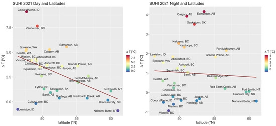
Figure 1.
SUHI intensity (ΔT) vs. latitude for 28 cities (Table 1) during the 2021 HW at daytime (left) and nighttime (right).
3.1.3. Interannual Variations on SUHI intensity
Results presented in the previous sections (Figure 1 and Figure S3) suggest that SUHI intensity does not necessarily increase during HWs. This finding is consistent with previous studies [86], while other studies even suggest a decrease in SUHI during HWs periods [87,88] or stay unchanged [89]. We calculated the mean SUHI over 28 cities (see Table 1) for the 2021 HW and also for sampling previous years (2000, 2002, and 2019) (Figure 2).
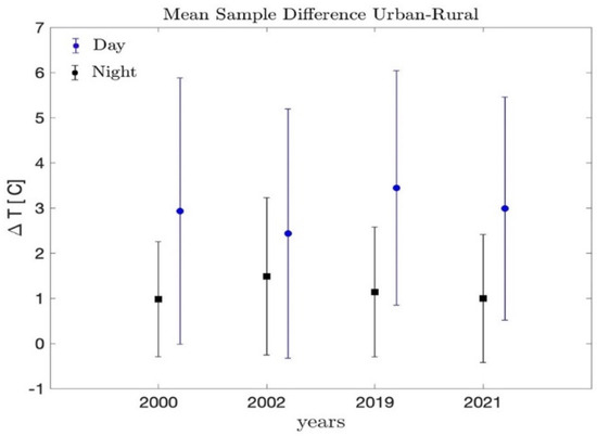
Figure 2.
A comparison of SUHI intensity averaged over the subset of 28 cities during the 2021 HW and previous years without HW. Standard deviation of the mean value is represented by vertical error bars.
Mean daytime SUHI values (with 1-sigma standard deviation) for years 2000, 2002, 2019, and 2021 were, respectively, 2.9 ± 2.9 °C, 2.4 ± 2.8 °C, 3.4 ± 2.6 °C, and 3.0 ± 2.5 °C. In the case of nighttime SUHI, mean values for years 2000, 2002, 2019, and 2021 were, respectively, 1.0 ± 1.3 °C, 1.5 ± 1.7 °C, 1.1 ± 1.4 °C, and 1.0 ± 1.4 °C. Such a comparative analysis of the mean SUHI intensity between HW and NHW periods (for the same date) suggests that HW did not increase SUHI intensity, despite the record LSTs values reached during this HW (Table 1). Moreover, previous years in absence of HW, with much lower LSTs, presented higher SUHI intensity than during the HW period. Therefore, the mean SUHI intensity experienced almost no influence of the HW. However, special attention to the differences per cities and towns shows that dissimilar trends within the sample occurs, probably due the potential influence of factors such as the interactions between the background climate with intraurban LULC, the latitude of the cities and towns’ location, and their degree of urbanization, etc.
3.1.4. Spatial Patterns of SUHI Intensity
Mapping the spatial patterns of SUHI intensity at urban scale constitutes a mean to better depict potential alterations and hotspots at intraurban spaces due to LC distribution as well as different structures of urban morphology. It is possible to identify general trends at the urban space by comparing MODIS LST data and MODIS true color composites maps, although given the very low spatial resolution of MODIS LST product (1 km) and the resolution of MODIS true color composites (500 m), the distinction of intraurban variability is highly restricted. However, the coarse resolution of MODIS still enables distinguishing some features over big cities (Figure 3). Visual analysis of MODIS maps of SUHI intensity enables visualizing a general trend indicating much higher SUHI values at intraurban space hotspots are located at regions of pixels with much higher averages of densely built-up areas, while regions of pixels with a higher share of urban green spaces and dense vegetation show lower LST values. This analysis will be further described by employing high spatial resolution Landsat-8 derived LST data in the following section.
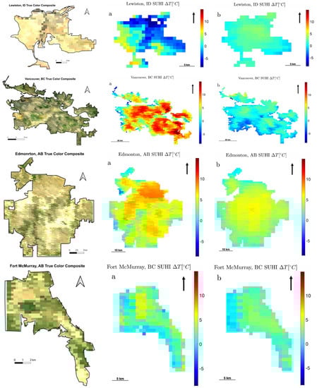
Figure 3.
MODIS true color composite maps (left column, 500 m) and MODIS SUHI intensity (central and right column 1 km): a. daytime and b. nighttime over Lewiston, Vancouver, Edmonton, and Fort McMurray cities for the 26 June 2021.
3.2. Analysis of SUHI from Landsat-8 Data
3.2.1. SUHI Intensity during the 2021 HW
The analysis of the sample of 18 selected cities and towns for Landsat-8 data has shown a mean urban LST of 40.6 ± 7.4 °C, a mean rural LST 35.1 ± 9.6 °C, and a mean SUHI intensity of 5.5 ± 6.1 °C (Table 4). SUHI values were typically positive (urban LSTs higher than rural LSTs), with exceptionally high values over Kamloops and Kelowna (SUHI values around +15 °C). Only four cities (in Canada: Ashcroft, BC; Beaverlodge, AB; Grande Prairie, AB; and in the U.S.: Lewiston, ID) provided negative values of SUHI.
Table 4.
Landsat-8 data for the sample of 18 cities: urban LSTs, rural LSTs, and SUHI intensity.
The comparison between daytime SUHI values estimated from MODIS data and Landsat-8 (Table S3) differs in magnitude, but it shows an overall high positive correlation (Pearson’s linear correlation coefficient of 0.86) (Figure 4). SUHI values estimated with Landsat-8 are higher than values estimated from MODIS. However, in some cases MODIS and Landsat-8 estimations of SUHI provided opposite results and/or huge discrepancies. This may not only be attributed to different spatial resolutions (1 km vs. 100 m) but also to the different dates of SUHI estimation. Due to the temporal resolution of Landsat-8 (16-day revisit time), in some cases, SUHI analysis was performed in different dates than those of MODIS data.
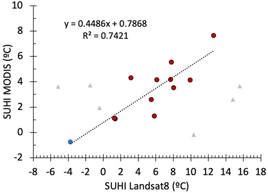
Figure 4.
Comparison between daytime SUHI intensities estimated from MODIS and Landsat-8 imagery for the subset of 18 cities (see also Table S3). Triangle symbols indicate outliers that were not considered in the linear fit.
3.2.2. Spatial Patterns of SUHI
The higher resolution of Landsat-8 imagery enables a more precise detection of hotspots with greater SUHI intensity at densely built-up locations and ISA without vegetation, while dense vegetation and water bodies show lower SUHI intensity (Figure 5). Grassland and bare soil present diverse results, showing cases of high as well as low SUHI intensity probably due to degree of grassland density and the soil type together with background microclimate. Mixed LC combining low-density built-up areas with vegetation shows moderate SUHI intensity. It is possible to infer that vegetation density appears to be functioning as a substantial attenuating factor of SUHI intensity when intertwined withing built-up areas.
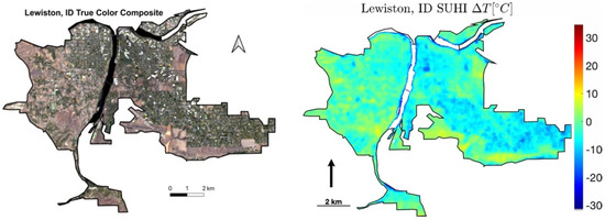

Figure 5.
True color RGB composition maps and daytime SUHI intensity (ΔT) for four sample cities: Lewiston, Vancouver, Edmonton, and Fort McMurray.
As expected, LST patterns follow that of SUHI (Figure S4). LST Maps indicate a visual association between lower LST values at vegetated areas and water bodies and higher LST values at either densely built-up areas or in some cases bare soil. A strong contrast was observed between dense vegetation associated with very low LST values and degrees of built-up areas’ density associated with intermediate to high LST values. Mixed urban LCs, where low density built-up areas are interspersed with vegetation, are associated with intermediate LST values, denotating the effect of vegetation on LST reduction for built-up settings. A clear contrast in the thermal landscape was observed between non-vegetated densely built-up areas—with higher LST values—and built-up areas with interspersed vegetation—with medium LST values. Square pockets of vegetation (Figure S4b) considerably diminishes LST values. Although bare soil also tends to have higher LST values than vegetated areas, it strongly depends on the soil type and local microclimatic conditions. Non-vegetated areas of bare soil show much higher LST values than urbanized areas with low and dense built-up vegetation, and the presence of two pockets of vegetated areas with lower LST values was also observable.
3.2.3. Thermal Comfort Conditions and Spatial Clusters
Visual analysis of the UFTVI maps (Figure 6, and additional maps in Figure S4) evidences a clear link between the thermal impact caused by SUHI intensity on the urban environmental conditions and the different types of LC. At the global urban scale (Figure 6), UFTVI categories show consistency with the distribution of LC types and structures of urban morphology, with hotspots of much higher SUHI impact at densely built-up areas. In contrast, dense vegetation, urban green spaces, and water bodies show lower impact. The crucial role of vegetation on SUHI impact is evidenced through a progressive variation on UFTVI categories, ranging from “no” SUHI impact and “excellent” ecological conditions to “strongest” SUHI impact with “worst” ecological conditions. Intermediate degrees of SUHI impact were found associated with built-up areas with different density degrees of intertwined vegetation (Figure S4).
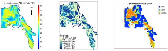
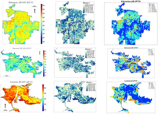
Figure 6.
Spatial patterns of LST, Local Moran’s I (MLI), and UFTVI using Landsat-8 data over the cities of Fort McMurray, Edmonton, Vancouver, and Lewiston.
Spatial patterns of SUHI (Figure 5) and LST (Figure 6) are qualitatively linked to LULC types. However, quantitative verification and analysis of LST spatial patterns require the application of geostatistical methods to verify if spatial patterns of LST exhibit clusters. The very high Moran’s I and very low Geary’s C values (with p-values < 0.001) obtained over the subset of 18 cities (Table S4) confirm the existence of clusters across the intraurban thermal landscape. Moreover, I coefficient values are close to 1, and C coefficient values are lower than 1, which indicates a highly positive spatial autocorrelation. Therefore, the results obtained in the geostatistical analysis led us to reject the null hypothesis (H0) of CSR or no autocorrelation. This unveils the existence of an ongoing spatial process behind such patterns. Such process at global levels quantitively demonstrates the extent at which LST patterns are spatially clustered. At a local level, it serves to identify LST clusters of localized hot spots and to verify whether a strong positive spatial correlation of urban impervious surfaces with higher LSTs or vegetated areas with lower LSTs exists. Moreover, contrariwise to traditional discrete categorical maps, the significance of spatial autocorrelation at local level mainly relies in mapping and detection of significant spatial clustering of homogeneous LST values occurring around a given observation. Furthermore, it serves for depicting the variability of the distribution of LST values across the urban space without losing the continuous gradient existing between them. These results are in agreement with previous research, which suggested the existence of LST clusters, as well as association between LST patterns, and ISA at intraurban spaces [51,52,53,54,55].
Visual analysis of the thermal landscape by using the MLI maps (Figure 6) allows us to infer that both lower and higher LST values tend to conform patterns of clusters of higher degree given their high MLI coefficient values. Thus, the clustering behavior of the urban thermal landscapes for the studied sample tends to show a clear trend in which classes of high clustering degree—with high MLI—occur at both lower and higher LST values. While intermediate vales of the thermal scale tend to present classes of lower clustering degree—given their lower MLI coefficient. Although the found trend is perceptible for both large (e.g., Vancouver and Edmonton in Figure 6) and medium to small-size cities (e.g., Fort McMurray and Lewiston in Figure 6), it is in the medium with respect to smaller cities and towns that clusters appear easier to visualize. This effect is due to the higher variability of the spatial distribution of LCs across the thermal landscape at larger cities, while medium to smaller cities and towns present a lower variability in their spatial distribution of LCs, therefore showing a continuous thermal landscape that tends to form larger spatial clusters. In the MLI map color scale, ranging from blue colors to yellow (Figure 6), the stronger the blue color, the higher the degree or strength of the cluster class, while the lighter the color, the lower the clustering degree of each of the classes. Note that the visual qualitative estimation of the lower, medium, and higher values of the thermal scale varies for each city, and this lack of normalization of the MLI map was purposely conducted in order to show changes in values found at each of the cities and towns of the sample and the abrupt variability that occurs as a function specific characteristic of the urban space and the thermal landscape. Such variability is not only due to the differences in the characteristics of LC types [117] but also results from specific topographic conditions [118] as well as the differences in latitudes of the sampled cities and towns, especially considering the largely extended area of North America covered by the sample (see Figure S1).
The analysis of clustering degree classes was further tested quantitively by employing scatterplots of the association between LST and MLI (Figure S5). These scatterplots showed a quadratic relationship between LST and MLI. The highest clustering degrees were found at the lowest LST values until reaching the vertex of the parabola; the latter functions as an inflection point located where the MLI coefficient value become 0. While an increasing clustering degree rises from the vertex until it reaches the height of LST values. The vertex as an inflection point between the two sides of the parabola’s axis of symmetry tends to vary its location at different LST values, which is in agreement with the range of LST values for the set of studied cities. These findings quantitively corroborate our hypothesis derived from the visual analysis of MLI maps (Figure 6) and scatterplots of LST vs. MLI (Figure S5), i.e., higher and lower LST values belong to classes of stronger clustering degree, while intermediate LST values belong to classes of weaker clustering degree.
4. Discussion
Many novel methodologies for estimating SUHI intensity aimed at the development of different indicators for the identification of non-urban (or rural) areas. These methodologies were based on the footprint LST-ISA relationship by means of Kernel Density Estimation (KDE) [119], local climate zone (LCZs) [120], ring-based buffer approach [121], surrounding reference regions [102], LC information [122], or nighttime light data [123], among others. However, a unified methodology that clearly defines non-urban areas has not yet been developed [102]. Moreover, urban areas as regions with higher shares of ISA with respect to non-urban areas have been defined with different methods across the literature [120,124,125,126]. Therefore, such methodological diversity and a lack of consensus in a clear definition of the apparent dichotomy between urban-rural and the sub-urban areas jeopardizes a robust comparison of SUHI studies over different regions and dates [120]. The difficulty involved in the definition of non-urban areas avoids the identification of a standardized universal method for estimating SUHI. This might be partly due to the current accelerated process of urbanization expansion and agglomeration, which has resulted in the emergence of very different landscape scenarios around cities. Hence, such interstitial spaces located beyond urban administrative borders and across its surroundings are composed of a heterogeneous mosaic of different landcovers, such as other urbanizations, forested areas, natural reserves, wildlands, and mixed spaces combining agriculture and bare soil with urbanizations. In this manner, peri-urban areas have become zones of transition for which is not always possible to automatically delineate a clear buffer zone composed mostly of pixels categorized as rural areas. The method followed in this research for estimating SUHI, inspired by the approach proposed by Sobrino and Irakulis, 2020 [102], provides an estimate of mean LST values of non-urban surrounding landscapes by carefully selecting external reference points with respect to the urban area based upon LC information of representative pixels, while avoiding potential extreme deviations of landscape scenarios.
Our results have shown that this HW presented the highest LST values for the last two decades (2000–2021) on the 26 June 2021. Extreme SUHI values were reached over particular regions, with values ranging from 5 to above 25 °C, with a mean daytime SUHI of 3.0 ± 2.5 °C and a mean nighttime of 1.0 ± 1.4 °C. However, we found that the HW did not intensify the SUHI effect for the expected values at such latitudes during summer.
As expected, an analysis of LST spatial patterns from remote sensing data has shown hotspots of much higher LST values at urban centers with densely built-up areas, whereas lower LST values were observed at urban green spaces and dense vegetation. High spatial resolution Landsat-8-derived LST (supported by Google Earth© information and RGB compositions) evidenced a strong contrast between higher and lower LST values at densely built-up areas and dense vegetation, respectively, while medium LST values dominated at mixed intraurban LC. In addition, we employed UFTVI to assess SUHI impacts on the thermal environmental quality and ecological conditions of the intraurban space. In agreement with previous findings [22,60,61,62], spatial patterns of UFTVI have shown the substantial role played by vegetation density in diminishing SUHI impact and reducing the thermal stress. UFTVI maps showed a clear association between LULC and SUHI intensity, and they were demonstrated to be a reliable indicator for depicting environmental thermal quality across different urban scales.
We evaluated the degree to which LST spatial distribution potentially exhibits organized patterns with similarly arranged values across the intraurban space, and we explored its variability during the occurrence of the HW by means of spatial autocorrelation indices. Thus, in line with Tobler’s first law of geography [127], which indicates that the strength of the spatial dependency [128] between values is based upon the distance relationship between them, attributing higher autocorrelation to closer values, we employed a geostatistical approach for cluster detection and analysis of the urban thermal landscape with high-resolution thermal remote sensing data. This approach, in agreement with the continuous landscape gradient model [129], allows the identification of groups of pixels with high homogeneity without overlooking the continuous gradient existing across landscapes in the geographic space. In this manner, we avoid potential loss of information that might result from discreet categorical models, providing an accurate representation of landscape heterogeneity.
Classified thematic maps of landscape patterns have been elaborated in other studies by using the discrete approach, which is based on contrasts with the continuous gradient paradigm. Following the discussion presented by Fan & Wang (2020) [51], although the “patch-mosaic” [47,48] modelling approach was mostly used for characterizing the composition and spatial configuration of LCs, it results in a discrete categorical description of landscapes by assuming different landscape features as homogenous units with sharply separated boundaries. However, at urban landscapes, this assumption tends to represent an unrealistic scenario due to the gradual variation encountered between patches. The discreet modeling approach relies on a subjective categorical definition of continuous landscape variables. Constructing sharp boundaries between discrete homogeneous classes results in the actual loss of relevant information, partly due to the removal of the intra-class variability [49,50]. For LST analysis, this approach tends to overlook the continuous nature of the progressive degrees in the distribution of LST values across the thermal landscape. Moreover, the discrete approach of landscape characterization based on traditional LC classifications has been questioned [130] due to uncertainties associated with LC classification accuracy estimations that can further be propagated. As explained by Shao and Wu (2008) [131], LULC maps derived from classified remote sensing data propagate errors derived from the estimators used to evaluate the accuracy of the classified thematic maps, which mainly are represented in terms of “producer’s accuracy,” “user’s accuracy,” and “overall accuracy”, that are commonly calculated from an error matrix or confusion matrix. There is no universal accepted standardized basis for quantifying the adequacy of such classification accuracy estimators, hence making the use of LULC maps questionable due to lack of a generally accepted threshold for classification accuracy. From a continuous landscape modelling approach, it is possible to rely on a signal that captures details in gradual variability or changes of the thermal landscape at pixel resolution. In this manner, we are looking at the urban thermal landscape as diverse groups or regions of LST values with internal homogeneity and external heterogeneity while viewing the continuous progressive degrees between clusters (e.g., the MLI maps in Figure 6).
We performed a quantitative analysis of the thermal landscape by employing geostatistical methods confirming the existence of clusters of LST values at the intraurban space. While employing MLI maps, clustering behavior was visualized, depicting the gradual continuous differentiation between adjacent clusters. MLI maps not only confirmed the visually observed spatial distribution of LST patterns but also revealed a clear trend with strong clustering at both lower and higher LST values while lower clustering degrees were found for intermediate LST values. Furthermore, a visual analysis of LST and MLI scatterplots has shown a quadratic relation. Results of polynomial regression with high R2 supported our hypothesis that higher and lower LST values belong to classes of stronger clustering degree, while intermediate LST values belong to classes of weaker clustering degree.
5. Conclusions
In this research, we employed TIR remotely sensed data with different spatial and temporal resolutions together with GIS data of urbanized areas for analyzing the impact of the last HW in Western North America on the magnitude of SUHI. We also analyzed the intraurban spatial distributions of LST patterns. Our results suggest that thermal remote sensing-derived LSTs with low spatial resolutions but with high temporal resolution and capability for capturing of day-night variations (MODIS) when coupled with high spatial resolution data (Landsat-8) together with geostatistical methods constitute a reliable means for analyzing spatial and temporal variations in LST with high accuracy. These results also demonstrate the significant contribution of LST as an indicator for analyzing the effects of SUHI intensity during HWs at urban scale. Although the HW over Western North America lasting from late June to mid-July 2021 registered the highest LST values for the last twenty-year period (2000–2021), we found that the SUHI in the studied sample of cities and towns was not intensified by the influence of HW. We found a clear trend indicating that SHUI intensity is higher at lower latitudes than higher latitudes for daytime, while such a clear trend does not hold for nighttime.
Some of the limitations of this study are a result of the polar orbit of the Landsat-8 satellite, with a temporal coverage interval of 16 days and, thus, time-restricted data provision, while the HW period lasted from late June to mid-July 2021. Consequently, the available number of images at high resolution was greatly reduced. In addition to the constraints of Landsat-8 data time resolution, due to its optical sensors, Landsat-8 clouded images over cities and towns, and the images were of inferior quality since they had a lower number of useful pixels. Cloud-contaminated pixels are known to frequently affect satellite thermal remote-sensing data used in SUHI studies [91]. In many cases, thin cloud coverage can contaminate images, making its detection even harder. We employed the MODIS 8-day LST product since it offers a window of 8 days in which if, for a given day images are clouded, the data of another day are taken within that window, the data provides greater data availability with regards to the MODIS-daily LST data product. This has increased the coverage of cities that we could study. However, a main drawback of using the MODIS 8-day LST product instead of the MODIS-daily LST product is that estimations cannot be performed for different dates within the 8-day time window.
These limitations may be better assessed or even overcome in the future by using daily TIR acquisitions with a more complete constellation of existing satellites (e.g., Sentinel-3, Suomi-NPP, etc.) and/or future TIR missions. It would be also valuable to compare the results obtained here with those of either previous or future HWs for the same and different climate zones, with consideration of urban morphology, vegetation density, and ISA coverage, together with background climate impact. This could serve to shed light on the still controversial complex effect of HWs on SHUI intensity.
Supplementary Materials
The following are available online at https://www.mdpi.com/article/10.3390/rs14030561/s1, Figure S1. Study area: a. US states and Canadian provinces comprising the 28 locations presenting highly pro-nounced LST values during the course of the heat wave the map’s projection corresponds to EPSG:3857-WGS 84/Pseudo-Mercator; b. Köppen-Geiger classification of climate zones of the US states and Canadian provinces highlighted in a. In order to preserve the native Coordinate Reference system (CRS) of the original Köppen-Geiger the map Figure S2b is presented in Geographic coordinates EPSG:4326 WGS 84; Figure S2. Daytime and nighttime LST (MODIS MOD11A2 product) time series over selected cities. The red dot indicates the maximum LST value; Figure S3. SUHI intensity (ΔT) vs. latitude for 28 cities (Table S1) for years 2000, 2002, and 2019 during daytime (left) and nighttime (right); Figure S4. Comparison between Google Map Satellite (left), LST (center), and UFTVI (right) maps over a zoomed area for four cities: (a) dense vegetation (very low LST) and medium to high built-up density (medium to high LST), (b) dense none-vegetated built-up area (high LST), built-up aeras interspersed with vegetation (medium LST), with a vegetated square (low LST), (c) bare soil (high LST), built-up aeras interspersed with vegetation (medium LST) also with pockets of vegetation (low LST), (d) dense vegetation (very low LST), none-vegetated built-up area (high LST), built-up aeras interspersed with vegetation (medium LST); Figure S5. Scatterplots of LST [°C] vs. MLI for some sample cities. A quadratic regression model, y = β0+β x +β x2+ ε, was assumed. The vertical dashed line marks the vertex of the parabola—point of inflection where LST values change from decreasing to increasing their clustering degree—while the horizontal dashed line marks where MLI is equal to 0 meaning no clustering is detected; Table S1. List of urbanized areas (cities and towns) distributed across continental U.S territories and Canada that were considered in this study. The subset of 28 cities that were analyzed from MODIS data are marked with an asterisk, while the subset of 18 cities that were analyzed from Landsat8 data are marked with a triangle. Population data was extracted from the US and Canada Census Bureau. Land area is given in km2; Table S2. Specifications of Landsat 8 data used in the analysis; Table S3. Comparison between SUHI intensities using MODIS (daytime) and Landsat 8 data; Table S4. Results of Global Mora’s I and Geary’s C for the sampled of 18 cities and towns studied.
Author Contributions
Conceptualization, methodology, and formal analysis, G.I.C. and J.C.J.; software, resources, and data curation, G.I.C.; writing—original draft preparation, G.I.C.; writing—review and editing, G.I.C. and J.C.J. All authors have read and agreed to the published version of the manuscript.
Funding
This research was partially supported by The Planning and Budgeting Committee (PBC) of the of the Israeli Council for Higher Education, through a grant awarded to the Data Science Research Center (DSRC) at the University of Haifa.
Data Availability Statement
Data used in this research are available upon reasonable request to the authors.
Conflicts of Interest
The authors declare no conflict of interest.
References
- Robinson, P.J. On the definition of a heat wave. J. Appl. Meteorol. 2001, 40, 762–775. [Google Scholar] [CrossRef]
- Lee, E.; Bieda, R.; Shanmugasundaram, J.; Basara Richter, H. Land surface and atmospheric conditions associated with heat waves over the Chickasaw Nation in the South Central United States. J. Geophys. Res. Atmos. 2016, 121, 6284–6298. [Google Scholar] [CrossRef]
- Guo, Y.; Gasparrini, A.; Armstrong, B.; Li, S.; Tawatsupa, B.; Tobias, A.; Lavigne, E.; Coelho, M.d.Z.S.; Leone, M.; Pan, X.; et al. Global variation in the effects of ambient temperature on mortality: A systematic evaluation. Epidemiology 2014, 25, 781–789. [Google Scholar] [CrossRef] [PubMed] [Green Version]
- Guirguis, K.; Gershunov, A.; Tardy, A.; Basu, R. The Impact of Recent Heat Waves on Human Health in California. J. Appl. Meteorol. Climatol. 2014, 53, 3–19. [Google Scholar] [CrossRef]
- Xia, Y.; Li, Y.; Guan, D.; Tinoco, D.M.; Xia, J.; Yan, Z.; Huo, H. Assessment of the economic impacts of heat waves: A case study of Nanjing, China. J. Clean. Prod. 2018, 171, 811–819. [Google Scholar] [CrossRef] [Green Version]
- Castillo, F.; Vargas, A.S.; Gilless, J.K.; Wehner, M. The Impact of Heat Waves on Agricultural Labor Productivity and Output. In Extreme Events and Climate Change: A Multidisciplanary Approach, 1st ed.; Castillo, F., Wehner, M., Stone, D.A., Eds.; John Wiley & Sons, Inc.: Hoboken, NJ, USA, 2021; pp. 11–20. [Google Scholar] [CrossRef]
- Dobricic, S.; Russo, S.; Pozzoli1, L.; Wilson, J.; Vignati, E. Increasing occurrence of heat waves in the terrestrial Arctic. Environ. Res. Lett. 2020, 15, 024022. [Google Scholar] [CrossRef]
- Lloret, F.; Batllori, E. Climate-Induced Global Forest Shifts due to Heatwave-Drought. Ecol. Stud. 2021, 241, 155–186. [Google Scholar] [CrossRef]
- Lansu, E.M.; Heerwaarden, C.C.; Stegehuis, A.I.; Teuling, A.J. Atmospheric Aridity and Apparent Soil Moisture Drought in European Forest During Heat Waves. Geophys. Res. Lett. 2020, 47, e2020GL087091. [Google Scholar] [CrossRef] [Green Version]
- Sutanto, S.J.; Vitolo, C.; Di Napoli, C.; D’Andrea, M.; Van Lanen, H.A.J. Heatwaves, droughts, and fires: Exploring compound and cascading dry hazards at the pan-European scale. Environ. Int. 2020, 134, 105276. [Google Scholar] [CrossRef]
- Mozny, M.; Trnka, M.; Brázdil, R. Climate change driven changes of vegetation fires in the Czech Republic. Theor. Appl. Climatol. 2020, 143, 691–699. [Google Scholar] [CrossRef]
- Albright, T.P.; Pidgeon, A.M.; Rittenhouse, C.D.; Clayton, M.K.; Flather, C.H.; Culbert, P.D.; Radeloff, V.C. Heat waves measured with MODIS land surface temperature data predict changes in avian community structure. Remote Sens. Environ. 2011, 115, 245–254. [Google Scholar] [CrossRef] [Green Version]
- Parmesan, C.; Yohe, G. A globally coherent fingerprint of climate change impacts across natural systems. Nature 2003, 421, 37–42. [Google Scholar] [CrossRef]
- Wernberg, T. Marine Heatwave Drives Collapse of Kelp Forests in Western Australia. Ecol. Stud. 2021, 241, 325–343. [Google Scholar] [CrossRef]
- Coumou, D.; Rahmstorf, S. A decade of weather extremes. Nat. Clim. Chang. 2012, 2, 491–496. [Google Scholar] [CrossRef]
- Guo, X.; Huang, J.; Luo, Y.; Zhao, Z.; Xu, Y. Projection of heat waves over China for eight different global warming targets using 12 CMIP5 models. Theor. Appl. Climatol. 2016, 128, 507–522. [Google Scholar] [CrossRef]
- Wu, X.; Wang, L.; Yao, R.; Luo, M.; Li, X. Identifying the dominant driving factors of heat waves in the North China Plain. Atmos. Res. 2021, 252, 105458. [Google Scholar] [CrossRef]
- Theeuwes, N.E.; Steeneveld, G.-J.; Ronda, R.J.; Rotach, M.W.; Holtslag, A.A.M. Cool city mornings by urban heat. Environ. Res. Lett. 2015, 10, 114022. [Google Scholar] [CrossRef]
- Oke, T.R. City Size and the Urban Heat Island. Atmos. Environ. 1973, 7, 769–779. [Google Scholar] [CrossRef]
- Oke, T.R. The Energetic Basis of the Urban Heat Island. Q. J. R. Met. Soc. 1982, 108, 1–24. [Google Scholar] [CrossRef]
- Santamouris, M.; Papanikolaou, N.; Livada, I.; Koronakis, I.; Georgakis, C.; Argiriou, A.; Assimakopoulos, D. On the impact of urban climate on the energy consumption of buildings. Sol. Energy 2001, 70, 201–216. [Google Scholar] [CrossRef]
- Saaroni, H.; Ben-Dor, E.; Bitan, A.; Potchter, O. Spatial distribution and microscale characteristics of the urban heat island in Tel-Aviv, Israel. Landsc. Urban Plan. 2000, 48, 1–18. [Google Scholar] [CrossRef]
- Hart, M.A.; Sailor, D.J. Quantifying the influence of land-use and surface characteristics on spatial variability in the urban heat island. Theor. Appl. Climatol. 2009, 95, 397–406. [Google Scholar] [CrossRef]
- Founda, D.; Santamouris, M. Synergies between Urban Heat Island and Heat Waves in Athens (Greece), during an extremely hot summer (2012). Sci. Rep. 2017, 7, 10973. [Google Scholar] [CrossRef] [PubMed] [Green Version]
- Zou, Z.; Yan, C.; Yu, L.; Jiang, X.; Ding, J.; Qin, L.; Qiu, G. Impacts of land use/ land cover types on interactions between urban heat island effects and heat waves. Build. Environ. 2021, 204, 108138. [Google Scholar] [CrossRef]
- Zhao, L.; Oppenheimer, M.; Zhu, Q.; Baldwin, J.W.; Ebi, K.L.; Bou-Zeid, E.; Liu, X. Interactions between urban heat islands and heat waves. Environ. Res. Lett. 2018, 13, 034003. [Google Scholar] [CrossRef]
- Pyrgou, A.; Hadjinicolaou, P.; Santamouris, M. Urban-rural moisture contrast: Regulator of the urban heat island and heatwaves’ synergy over a mediterranean city. Environ. Res. 2020, 182, 109102. [Google Scholar] [CrossRef] [PubMed]
- Shreevastava, A.; Prasanth, S.; Ramamurthy, P.; Rao, P.S.C. Scale-dependent response of the urban heat island to the European heatwave of 2018. Environ. Res. Lett. 2021, 16, 104021. [Google Scholar] [CrossRef]
- Kong, J.; Zhao, Y.; Carmeliet, J.; Lei, C. Urban Heat Island and Its Interaction with Heatwaves: A Review of Studies on Mesoscale. Sustainability 2021, 13, 10923. [Google Scholar] [CrossRef]
- Chapman, S.C.; Watkins, N.W.; Stainforth, D.A. Warming Trends in Summer Heatwaves. Geophys. Res. Lett. 2019, 46, 1634–1640. [Google Scholar] [CrossRef] [Green Version]
- Unkašević, M.; Tošić, I. Seasonal analysis of cold and heat waves in Serbia during the period 1949–2012. Theor. Appl. Climatol. 2014, 120, 29–40. [Google Scholar] [CrossRef]
- Li, Z.-L.; Tang, B.-H.; Wu, H.; Ren, H.; Yan, G.; Wan, Z.; Sobrino, J.A. Satellite-derived land surface temperature: Current status and perspectives. Remote Sens. Environ. 2013, 131, 14–37. [Google Scholar] [CrossRef] [Green Version]
- Bateni, S.M.; Entekhabi, D. Relative efficiency of land surface energy balance components. Water Resour. Res. 2012, 48, W04510. [Google Scholar] [CrossRef]
- Schwaab, J.; Meier, R.; Bürgi, C.; Mussetti, G.; Seneviratne, S.I.; Davin, E.L. The role of urban trees in reducing land surface temperatures in European cities. Nat. Commun. 2021, 12, 6763. [Google Scholar] [CrossRef] [PubMed]
- Bokaie, M.; Zarkesh, M.K.; Arasteh, P.D.; Hosseini, A. Assessment of Urban Heat Island based on the relationship between land surface temperature and Land Use/ Land Cover in Tehran. Sustain. Cities Soc. 2016, 23, 94–104. [Google Scholar] [CrossRef]
- Walawender, J.P.; Szymanowski, M.; Hajto, M.J.; Bokwa, A. Land Surface Temperature Patterns in the Urban Agglomeration of Krakow (Poland) Derived from Landsat-7/ETM+ Data. Pure Appl. Geophys. 2013, 171, 913–940. [Google Scholar] [CrossRef] [Green Version]
- Oke, T.R.; Mills, G.; Christen, A.; Voogt, J.A. Urban Climates; Cambridge University Press: Cambridge, UK, 2017. [Google Scholar]
- Martilli, A.; Krayenhoff, E.S.; Nazarian, N. Is the Urban Heat Island intensity relevant for heat mitigation studies? Urban Clim. 2020, 31, 100541. [Google Scholar] [CrossRef]
- Li, X.; Zhou, W.; Ouyang, Z.; Xu, W.; Zheng, H. Spatial pattern of greenspace affects land surface temperature: Evidence from the heavily urbanized Beijing metropolitan area, China. Landsc. Ecol. 2012, 27, 887–898. [Google Scholar] [CrossRef]
- Li, X.; Zhou, W.; Ouyang, Z. Relationship between land surface temperature and spatial pattern of greenspace: What are the effects of spatial resolution? Landsc. Urban Plan. 2013, 114, 1–8. [Google Scholar] [CrossRef]
- Zhou, W.; Huang, G.; Cadenasso, M.L. Does spatial configuration matter? Understanding the effects of land cover pattern on land surface temperature in urban landscapes. Landsc. Urban Plan. 2011, 102, 54–63. [Google Scholar] [CrossRef]
- Li, K.; Zhang, W. Directionally and spatially varying relationship between land surface temperature and land-use pattern considering wind direction: A case study in central China. Environ. Sci. Pollut. Res. 2021, 28, 44479–44493. [Google Scholar] [CrossRef]
- Rao, Y.; Dai, J.; Dai, D.; He, Q. Effect of urban growth pattern on land surface temperature in China: A multi-scale landscape analysis of 338 cities. Land Use Policy 2021, 103, 105314. [Google Scholar] [CrossRef]
- Abdulmana, S.; Lim, A.; Wongsai, S.; Wongsai, N. Land surface temperature and vegetation cover changes and their relationships in Taiwan from 2000 to 2020. Remote Sens. Appl. Soc. Environ. 2021, 24, 100636. [Google Scholar] [CrossRef]
- Effati, F.; Karimi, H.; Yavari, A. Investigating effects of land use and land cover patterns on land surface temperature using landscape metrics in the city of Tehran, Iran. Arab. J. Geosci. 2021, 14, 1240. [Google Scholar] [CrossRef]
- Yu, Z.; Zhang, J.; Yang, G.; Schlaberg, J. Reverse Thinking: A New Method from the Graph Perspective for Evaluating and Mitigating Regional Surface Heat Islands. Remote Sens. 2021, 13, 1127. [Google Scholar] [CrossRef]
- Forman, R.T.T. Land Mosaics: The Ecology of Landscapes and Regions; Cambridge University Press: Cambridge, UK, 1995. [Google Scholar]
- Turner, M.G.; Gardner, R.H.; O’Neill, R.V. Landscape Ecology in Teory and Practice; Springer: Berlin/Heidelberg, Germany, 2001. [Google Scholar]
- Southworth, J.; Munroe, D.; Nagendra, H. Land cover change and landscape fragmentation—Comparing the utility of continuous and discrete analyses for a western Honduras region. Agric. Ecosyst. Environ. 2004, 101, 185–205. [Google Scholar] [CrossRef]
- Wulder, M.; Boots, B. Local spatial autocorrelation characteristics of remotely sensed imagery assessed with the Getis statistic. Int. J. Remote Sens. 1998, 19, 2223–2231. [Google Scholar] [CrossRef]
- Fan, C.; Wang, Z. Spatiotemporal Characterization of Land Cover Impacts on Urban Warming: A Spatial Autocorrelation Approach. Remote Sens. 2020, 12, 1631. [Google Scholar] [CrossRef]
- Kumari, M.; Sarma, K.; Sharma, R. Using Moran’s I and GIS to study the spatial pattern of land surface temperature in relation to land use/cover around a thermal power plant in Singrauli district, Madhya Pradesh, India. Remote Sens. Appl. Soc. Environ. 2019, 15, 100239. [Google Scholar] [CrossRef]
- Portela, C.I.; Massi, K.G.; Rodrigues, T.; Alcântara, E. Impact of urban and industrial features on land surface temperature: Evidences from satellite thermal indices. Sustain. Cities Soc. 2020, 56, 102100. [Google Scholar] [CrossRef]
- Das Majumdar, D.; Biswas, A. Quantifying land surface temperature change from LISA clusters: An alternative approach to identifying urban land use transformation. Landsc. Urban Plan. 2016, 153, 51–65. [Google Scholar] [CrossRef]
- Wu, X.; Li, B.; Li, M.; Guo, M.; Zang, S.; Zhang, S. Examining the Relationship Between Spatial Configurations of Urban Impervious Surfaces and Land Surface Temperature. Chin. Geogr. Sci. 2019, 29, 568–578. [Google Scholar] [CrossRef] [Green Version]
- Cao, X.; Onishi, A.; Chen, J.; Imura, H. Quantifying the cool island intensity of urban parks using ASTER and IKONOS data. Landsc. Urban Plan. 2010, 96, 224–231. [Google Scholar] [CrossRef]
- Shishegar, N. The Impacts of Green Areas on Mitigating Urban Heat Island Effect. Int. J. Environ. Sustain. 2014, 9, 119–130. [Google Scholar] [CrossRef]
- Ren, Z.; He, X.; Zheng, H.; Zhang, D.; Yu, X.; Shen, G.; Guo, R. Estimation of the Relationship between Urban Park Characteristics and Park Cool Island Intensity by Remote Sensing Data and Field Measurement. Forests 2013, 4, 868–886. [Google Scholar] [CrossRef] [Green Version]
- Ben-Dor, E.; Saaroni, H. Airborne video thermal radiometry as a tool for monitoring microscale structures of the urban heat island. Int. J. Remote Sens. 1997, 18, 3039–3053. [Google Scholar] [CrossRef]
- Shashua-Bar, L.; Hoffman, M.E. Vegetation as a climatic component in the design of an urban street An empirical model for predicting the cooling effect of urban green. Energy Build. 2000, 31, 221–235. [Google Scholar] [CrossRef]
- Shashua-Bar, L.; Potchter, O.; Bitan, A.; Boltansky, D.; Yaakov, Y. Microclimate modelling of street tree species effects within the varied urban morphology in the Mediterranean city of Tel Aviv. Israel. Int. J. Climatol. 2010, 30, 44–57. [Google Scholar] [CrossRef]
- Shashua-Bar, L.; Pearlmutter, D.; Erell, E. The influence of trees and grass on outdoor thermal comfort in a hot-arid environment. Int. J. Climatol. 2011, 31, 1498–1506. [Google Scholar] [CrossRef]
- Mijani, N.; Alavipanah, S.K.; Hamzeh, S.; Firozjaei, M.K.; Arsanjani, J.J. Modeling thermal comfort in different condition of mind using satellite images: An Ordered Weighted Averaging approach and a case study. Ecol. Indic. 2019, 104, 1–12. [Google Scholar] [CrossRef]
- Feng, L.; Zhao, M.; Zhou, Y.; Zhu, L.; Tian, H. The seasonal and annual impacts of landscape patterns on the urban thermal comfort using Landsat. Ecol. Indic. 2020, 110, 105798. [Google Scholar] [CrossRef]
- Zhang, Y.; Yu, T.; Gu, X.; Zhang, Y.; Chen, L. Land surface temperature retrieval from CBERS-02 IRMSS thermal infrared data and its applications in quantitative analysis of urban heat island effect. J. Remote Sens. 2006, 10, 789. [Google Scholar]
- Liu, L.; Zhang, Y. Urban Heat Island Analysis Using the Landsat TM Data and ASTER Data: A Case Study in Hong Kong. Remote Sens. 2011, 3, 1535–1552. [Google Scholar] [CrossRef] [Green Version]
- Naim, M.N.H.; Kafy, A.A. Assessment of urban thermal field variance index and defining the relationship between land cover and surface temperature in Chattogram city: A remote sensing and statistical approach. Environ. Chall. 2021, 4, 100107. [Google Scholar] [CrossRef]
- Singh, P.; Kikon, N.; Verma, P. Impact of land use change and urbanization on urban heat island in Lucknow city, Central India. A remote sensing based estimate. Sustain. Cities Soc. 2017, 32, 100–114. [Google Scholar] [CrossRef]
- Faisal, A.A.; Kafy, A.A.; Al Rakib, A.; Akter, K.S.; Jahir, D.M.A.; Sikdar, M.S.; Rahman, M.M. Assessing and predicting land use/land cover, land surface temperature and urban thermal field variance index using Landsat imagery for Dhaka Metropolitan area. Environ. Chall. 2021, 4, 100192. [Google Scholar] [CrossRef]
- Guha, S. Dynamic seasonal analysis on LST-NDVI relationship and ecological health of Raipur City, India. Ecosyst. Health Sustain. 2021, 7, 1927852. [Google Scholar] [CrossRef]
- Nguyen, T.; Lin, T.-H.; Chan, H.-P. The Environmental Effects of Urban Development in Hanoi, Vietna from Satellite and Meteorological Observations from 1999–2016. Sustainability 2019, 11, 1768. [Google Scholar] [CrossRef] [Green Version]
- Hung, T.; Uchihama, D.; Ochi, S.; Yasuoka, Y. Assessment with satellite data of the urban heat island effects in Asian mega cities. Int. J. Appl. Earth Obs. Geoinf. 2006, 8, 34–48. [Google Scholar] [CrossRef]
- Weng, Q.; Lu, D.; Schubring, J. Estimation of land surface temperature–vegetation abundance relationship for urban heat island studies. Remote Sens. Environ. 2004, 89, 467–483. [Google Scholar] [CrossRef]
- Li, D.; Bou-Zeid, E. Synergistic Interactions between Urban Heat Islands and Heat Waves: The Impact in Cities Is Larger than the Sum of Its Parts. J. Appl. Meteorol. Climatol. 2013, 52, 2051–2064. [Google Scholar] [CrossRef] [Green Version]
- Mildrexler, D.J.; Zhao, M.; Cohen, W.B.; Running, S.W.; Song, X.P.; Jones, M.O. Thermal Anomalies Detect Critical Global Land Surface Changes. J. Appl. Meteorol. Climatol. 2018, 57, 391–411. [Google Scholar] [CrossRef]
- Yan, Y.; Mao, K.; Shi, J.; Piao, S.; Shen, X.; Dozier, J.; Bao, Q. Driving forces of land surface temperature anomalous changes in North America in 2002–2018. Sci. Rep. 2020, 10, 6931. [Google Scholar] [CrossRef] [PubMed]
- Ossola, A.; Jenerette, G.D.; McGrath, A.; Chow, W.; Hughes, L.; Leishman, M.R. Small vegetated patches greatly reduce urban surface temperature during a summer heatwave in Adelaide, Australia. Landsc. Urban Plan. 2021, 209, 104046. [Google Scholar] [CrossRef]
- Dousset, B.; Gourmelon, F.; Laaidi, K.; Zeghnoun, A.; Giraudet, E.; Bretin, P.; Vandentorren, S. Satellite monitoring of summer heat waves in the Paris metropolitan area. Int. J. Climatol. 2010, 31, 313–323. [Google Scholar] [CrossRef]
- Cheval, S.; Dumitrescu, A.; Bell, A. The urban heat island of Bucharest during the extreme high temperatures of July 2007. Theor. Appl. Climatol. 2009, 97, 391–401. [Google Scholar] [CrossRef]
- Tomlinson, C.J.; Chapman, L.; Thornes, J.E.; Baker, C.J. Derivation of Birmingham’s summer surface urban heat island from MODIS satellite images. Int. J. Climatol. 2012, 32, 214–224. [Google Scholar] [CrossRef] [Green Version]
- Rizvi, S.H.; Alam, K.; Iqbal, M.J. Spatio-temporal variations in urban heat island and its interaction with heat wave. J. Atmos. Sol.-Terr. Phys. 2019, 185, 50–57. [Google Scholar] [CrossRef]
- Zhou, Y.; Shepherd, J.M. Atlanta’s urban heat island under extreme heat conditions and potential mitigation strategies. Nat. Hazards 2010, 52, 639–668. [Google Scholar] [CrossRef]
- Zaitchik, B.F.; Macalady, A.K.; Bonneau, L.R.; Smith, R.B. Europe’s 2003 heat wave: A satellite view of impacts and land–atmosphere feedbacks. Int. J. Climatol. 2006, 26, 743–769. [Google Scholar] [CrossRef]
- Ward, K.; Lauf, S.; Kleinschmit, B.; Endlicher, W. Heat waves and urban heat islands in Europe: A review of relevant drivers. Sci. Total Environ. 2016, 569–570, 527–539. [Google Scholar] [CrossRef]
- Oliveira, A.; Lopes, A.; Correia, E.; Niza, S.; Soares, A. Heatwaves and Summer Urban Heat Islands: A Daily Cycle Approach to Unveil the Urban Thermal Signal Changes in Lisbon, Portugal. Atmosphere 2021, 12, 292. [Google Scholar] [CrossRef]
- Scott, A.A.; Waugh, D.W.; Zaitchik, B.F. Reduced Urban Heat Island intensity under warmer conditions. Environ. Res. Lett. 2018, 13, 064003. [Google Scholar] [CrossRef] [PubMed]
- Richard, Y.; Pohl, B.; Rega, M.; Pergaud, J.; Thevenin, T.; Emery, J.; Dudek, J.; Vairet, T.; Zito, S.; Chateau-Smith, C. Is Urban Heat Island intensity higher during hot spells and heat waves (Dijon, France, 2014–2019)? Urban Clim. 2021, 35, 100747. [Google Scholar] [CrossRef]
- Kumar, R.; Mishra, V. Decline in surface urban heat island intensity in India during heatwaves. Environ. Res. Commun. 2019, 1, 031001. [Google Scholar] [CrossRef] [Green Version]
- Chew, L.W.; Liu, X.; Li, X.-X.; Norford, L.K. Interaction between heat wave and urban heat island: A case study in a tropical coastal city, Singapore. Atmos. Res. 2021, 247, 105134. [Google Scholar] [CrossRef]
- Sjoukje, Y.P.; Kew, S.F.; van Oldenborgh, G.J.; Anslow, F.S.; Seneviratne, S.I.; Vautard, R.; Coumou, D.; Ebi, K.L.; Arrighi, J.; Singh, R.; et al. Rapid Attribution Analysis of the Extraordinary Heatwave on the Pacific Coast of the US and Canada June 2021. World Weather Attribution. Available online: https://www.worldweatherattribution.org/wp-content/uploads/NW-US-extreme-heat-2021-scientific-report-WWA.pdf (accessed on 3 September 2021).
- Zhou, D.; Xiao, J.; Bonafoni, S.; Berger, C.; Deilami, K.; Zhou, Y.; Sobrino, J. Satellite Remote Sensing of Surface Urban Heat Islands: Progress, Challenges, and Perspectives. Remote Sens. 2018, 11, 48. [Google Scholar] [CrossRef] [Green Version]
- Beck, H.E.; Zimmermann, N.E.; McVicar, T.R.; Vergopolan, N.; Berg, A.; Wood, E.F. Present and future Köppen-Geiger climate classification maps at 1-km resolution. Sci. Data 2018, 5, 180214. [Google Scholar] [CrossRef] [Green Version]
- Available online: https://www.census.gov/geographies/mapping-files/time-series/geo/carto-boundary-file.2017.html (accessed on 8 September 2021).
- Available online: https://www12.statcan.gc.ca/census-recensement/2011/geo/bound-limit/bound-limit-2016-eng.cfm (accessed on 8 September 2021).
- Available online: https://lpdaac.usgs.gov/products/mod11a2v006/ (accessed on 8 September 2021).
- Available online: https://lpdaac.usgs.gov/products/mod09gav006/ (accessed on 11 November 2021).
- Available online: https://earthexplorer.usgs.gov (accessed on 8 September 2021).
- Roy, D.P.; Wulder, M.; Loveland, T.R.; Woodcock, C.; Allen, R.; Anderson, M.; Helder, D.; Irons, J.; Johnson, D.; Kennedy, R. Landsat-8: Science and product vision for terrestrial global change research. Remote Sens. Environ. 2014, 145, 154–172. [Google Scholar] [CrossRef] [Green Version]
- Xu, H. Modification of Normalized Difference Water Index (NDWI) to Enhance Open Water Features in Remotely Sensed Imagery. Int. J. Remote Sens. 2006, 27, 3025–3033. [Google Scholar] [CrossRef]
- Ko, B.; Kim, H.; Nam, J. Classification of Potential Water Bodies Using Landsat 8 OLI and a Combination of Two Boosted Random Forest Classifiers. Sensors 2015, 15, 13763–13777. [Google Scholar] [CrossRef] [Green Version]
- USGS (United States Geological Survey). Landsat 8 Collection 2 (C2) Level 2 Science Product (L2SP) Guide; Department of the Interior US Geological Survey: Reston, VA, USA, 2020.
- Sobrino, J.A.; Irakulis, I. A Methodology for Comparing the Surface Urban Heat Island in Selected Urban Agglomerations Around the World from Sentinel-3 SLSTR Data. Remote Sens. 2020, 12, 2052. [Google Scholar] [CrossRef]
- Goodchild, M.F.; Openshaw, S. Algorithm 9: Simulation of Autocorrelation for Aggregate Data. Environ. Plan. A Econ. Space 1980, 12, 1073–1081. [Google Scholar] [CrossRef]
- Goodchild, M.F. Spatial Autocorrelation; CATMOG 47; Geo Books: Norwich, UK, 1986. [Google Scholar]
- Zhou, X.; Lin, H. Geary’s, C. In Encyclopedia of GIS; Shekhar, S., Xiong, H., Zhou, X., Eds.; Springer: Cham, Switherland, 2017. [Google Scholar] [CrossRef]
- Bivand, R.; Pebesma, E.; Gomez-Rubio, V. Applied Spatial Data Analysis with R, 2nd ed.; Springer: New York, NY, USA, 2013; pp. 281–282. [Google Scholar]
- Bivand, R.; Wong, D.W.S. Comparing implementations of global and local indicators of spatial association. Test 2018, 27, 716–748. [Google Scholar] [CrossRef]
- Anselin, L. Local indicators of spatial association: LISA. Geogr. Anal. 1995, 27, 93–115. [Google Scholar] [CrossRef]
- How Do I Use a Scale Factor with Landsat Level-2 Science Products? USGS Mapping, Remote Sensing and Geospatial Data. Available online: https://www.usgs.gov/faqs/how-do-i-use-a-scale-factor-landsat-level-2-science-products?qt-news_science_products=0#qt-news_science_products (accessed on 8 September 2021).
- QGIS Development Team. QGIS Version 3.18. Geographic Information System. Open-Source Geospatial Foundation Project. 2021. Available online: https://www.qgis.org/en/site/ (accessed on 9 August 2021).
- MathWorks. MATLAB ver. 2021b Computer Program; The MathWorks Inc.: Natick, MA, USA, 2021; Available online: https://www.mathworks.com/ (accessed on 9 August 2021).
- R Core Team. R: A Language and Environment for Statistical Computing; Version 4.1.1.; R Foundation for Statistical Computing: Vienna, Austria, 2021; Available online: https://www.R-project.org/ (accessed on 9 August 2021).
- Bivand, R. Spdep: Spatial Dependence: Weighting Schemes, Statistics and Models. R Package Version 1.1-11. 2021. Available online: http://CRAN.R-project.org/package=spdep (accessed on 9 August 2021).
- Hijmans, R.J.; Van Etten, J. Raster: Geographic Analysis and Modeling with Raster Data. R Package Version 3.5-2. 2021. Available online: http://CRAN.R-project.org/package=raster (accessed on 9 August 2021).
- Tennekes, M. tmap: Thematic Maps in R. J. Stat. Softw. 2018, 84, 1–39. [Google Scholar] [CrossRef] [Green Version]
- Available online: https://gis.ncdc.noaa.gov/maps/ncei/summaries/daily (accessed on 8 September 2021).
- Tan, J.; Yu, D.; Li, Q.; Tan, X.; Zhou, W. Spatial relationship between land-use/land-cover change and land surface temperature in the Dongting Lake area, China. Sci. Rep. 2020, 10, 9245. [Google Scholar] [CrossRef]
- Peng, X.; Wu, W.; Zheng, Y.; Sun, J.; Hu, T.; Wang, P. Correlation analysis of land surface temperature and topographic elements in Hangzhou, China. Sci. Rep. 2020, 10, 10451. [Google Scholar] [CrossRef]
- Li, H.; Zhou, Y.; Li, X.; Meng, L.; Wang, X.; Wu, S.; Sodoudi, S. A new method to quantify surface urban heat island intensity. Sci. Total Environ. 2018, 624, 262–272. [Google Scholar] [CrossRef] [PubMed]
- Stewart, I.D.; Oke, T.R. Local climate zones for urban temperature studies. Bull. Am. Meteorol. Soc. 2012, 93, 1879–1900. [Google Scholar] [CrossRef]
- Bonafoni, S.; Keeratikasikorn, C. Land surface temperature and urban density: Multiyear modeling and relationship analysis using MODIS and Landsat data. Remote Sens. 2018, 10, 1471. [Google Scholar] [CrossRef] [Green Version]
- Sobrino, J.; Oltra-Carrió, R.; Sòria, G.; Jiménez-Muñoz, J.C.; Franch, B.; Hidalgo, V.; Mattar, C.; Julien, Y.; Cuenca, J.; Romaguera, M.; et al. Evaluation of the surface urban heat island effect in the city of Madrid by thermal remote sensing. Int. J. Remote Sens. 2013, 34, 3177. [Google Scholar] [CrossRef]
- Li, J.; Wang, F.; Fu, Y.; Guo, B.; Zhao, Y.; Yu, H. A Novel SUHI Referenced Estimation Method for Multicenters Urban Agglomeration using DMSP/OLS Nighttime Light Data. IEEE J. Sel. Top. Appl. Earth Obs. Remote Sens. 2020, 13, 1416–1425. [Google Scholar] [CrossRef]
- Peng, J.; Ma, J.; Liu, Q.; Liu, Y.; Hu, Y.; Li, Y.; Yue, Y. Spatial-temporal change of land surface temperature across 285 cities in China: An urban-rural contrast perspective. Sci. Total Environ. 2018, 635, 487–497. [Google Scholar] [CrossRef]
- Imhoff, M.L.; Zhang, P.; Wolfe, R.E.; Bounoua, L. Remote sensing of the urban heat island effect across biomes in the continental USA. Remote Sens. Environ. 2010, 114, 504–513. [Google Scholar] [CrossRef] [Green Version]
- Zhou, D.; Zhao, S.; Liu, S.; Zhang, L.; Zhu, C. Surface urban heat island in China’s 32 major cities: Spatial patterns and drivers. Remote Sens. Environ. 2014, 152, 51–61. [Google Scholar] [CrossRef]
- Tobler, W.R. A Computer Movie Simulating Urban Growth in the Detroit Region. Econ. Geogr. 1970, 46, 234. [Google Scholar] [CrossRef]
- Gangodagamage, C.; Zhou, X.; Lin, H. Autocorrelation, Spatial. In Encyclopedia of GIS; Shekhar, S., Xiong, H., Eds.; Springer: Boston, MA, USA, 2008. [Google Scholar] [CrossRef]
- McGarigal, K.; Cushman, S. The gradient concept of landscape structure [Chapter 12]. In Issues and Perspectives in Landscape Ecology; Wiens, J.A., Moss, M.R., Eds.; Cambridge University Press: Cambridge, UK, 2005; pp. 112–119. [Google Scholar]
- Fan, C.; Myint, S. A comparison of spatial autocorrelation indices and landscape metrics in measuring urban landscape fragmentation. Landsc. Urban Plan. 2014, 121, 117–128. [Google Scholar] [CrossRef]
- Shao, G.; Wu, J. On the accuracy of landscape pattern analysis using remote sensing data. Landsc. Ecol. 2008, 23, 505–511. [Google Scholar] [CrossRef]
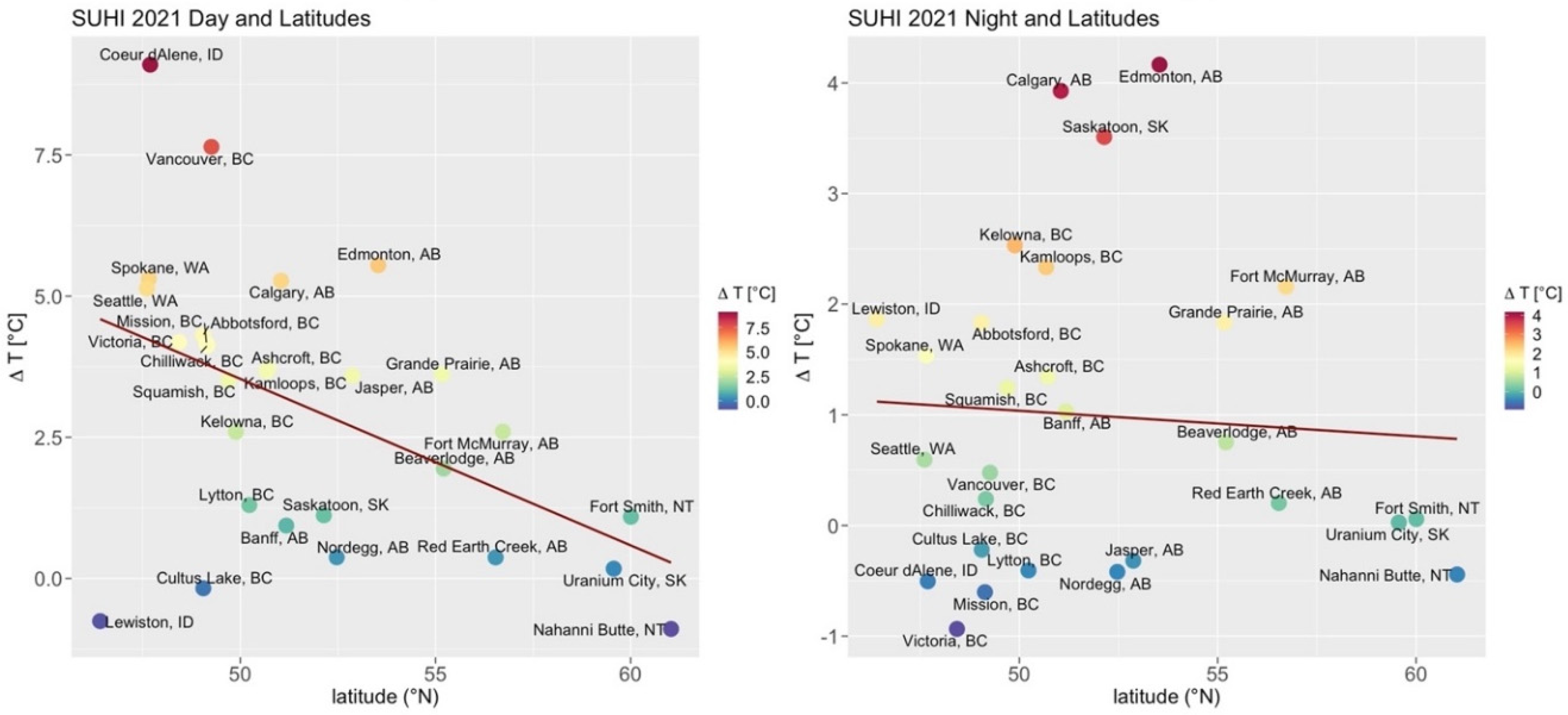
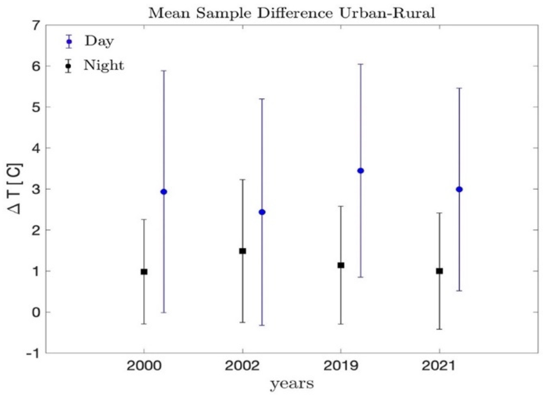

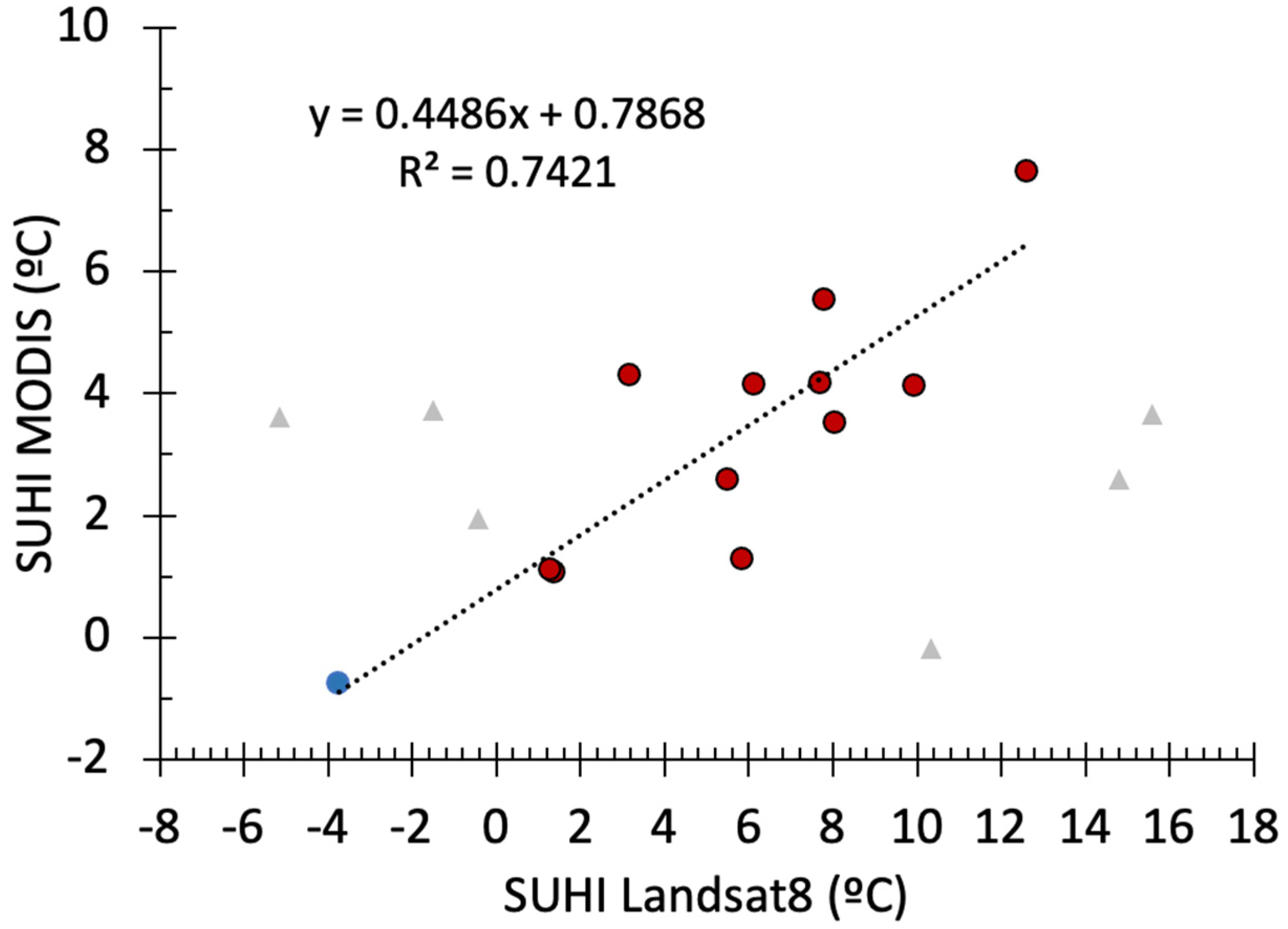
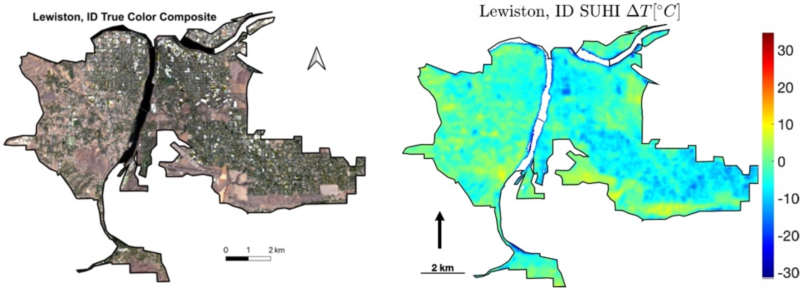
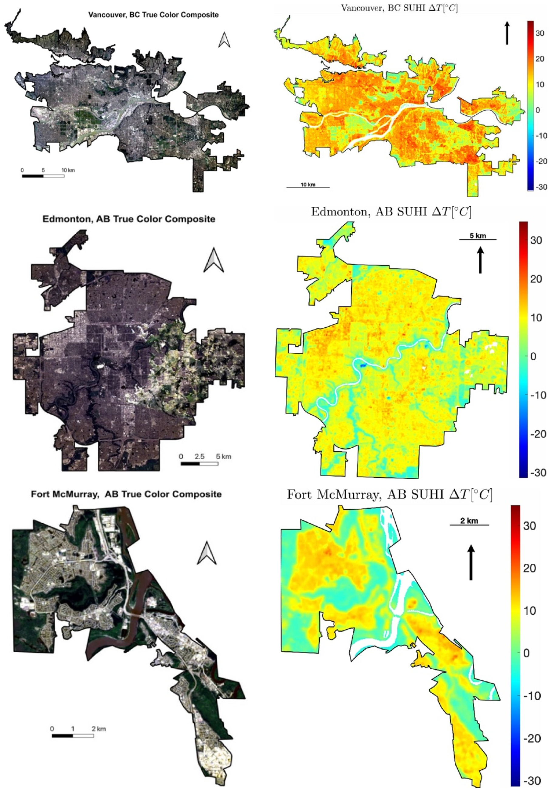
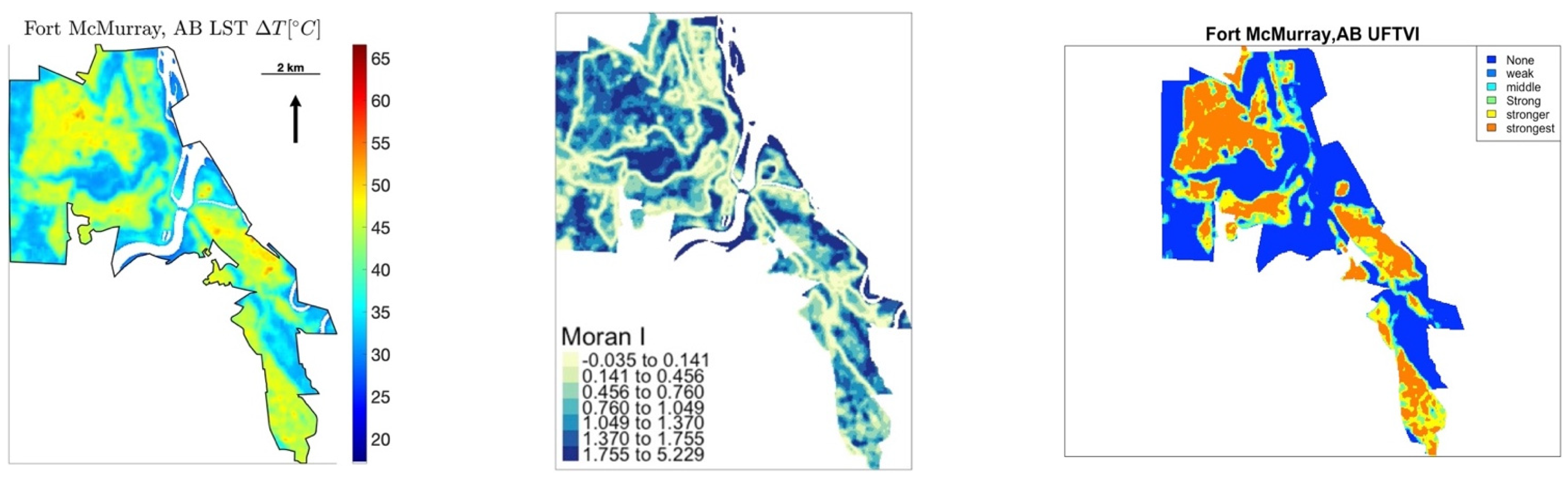

Publisher’s Note: MDPI stays neutral with regard to jurisdictional claims in published maps and institutional affiliations. |
© 2022 by the authors. Licensee MDPI, Basel, Switzerland. This article is an open access article distributed under the terms and conditions of the Creative Commons Attribution (CC BY) license (https://creativecommons.org/licenses/by/4.0/).