
Smallholder Crop Type Mapping and Rotation Monitoring in Mountainous Areas with Sentinel-1/2 Imagery


Abstract
:1. Introduction
2. Data and Methods
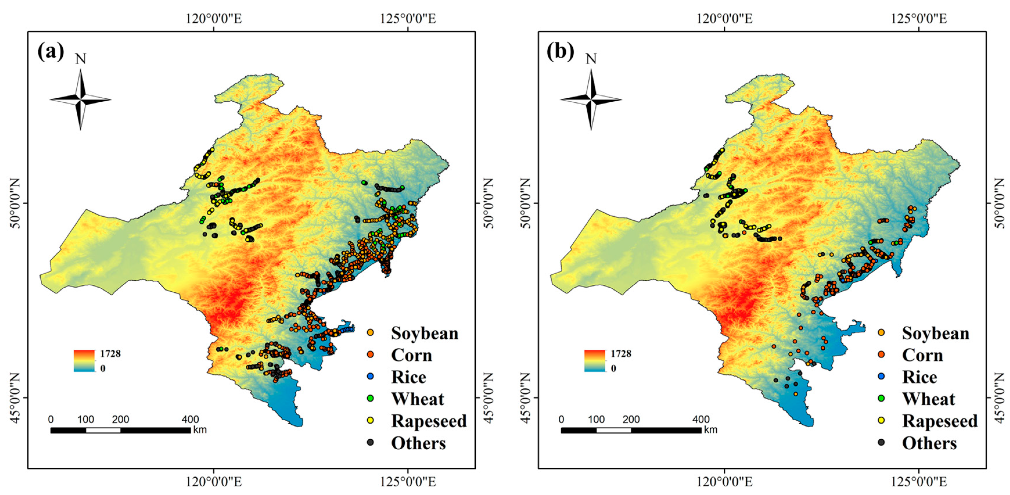
2.1. Study Area
2.2. Data and Processing
2.2.1. Sentinel-1 Imagery and Preprocessing
2.2.2. Sentinel-2 Imagery and Preprocessing
2.2.3. Cropland Layer Mask
2.3. Crop Type Reference Data
2.4. Crop Type Classification
2.5. Accuracy Assessment
3. Results
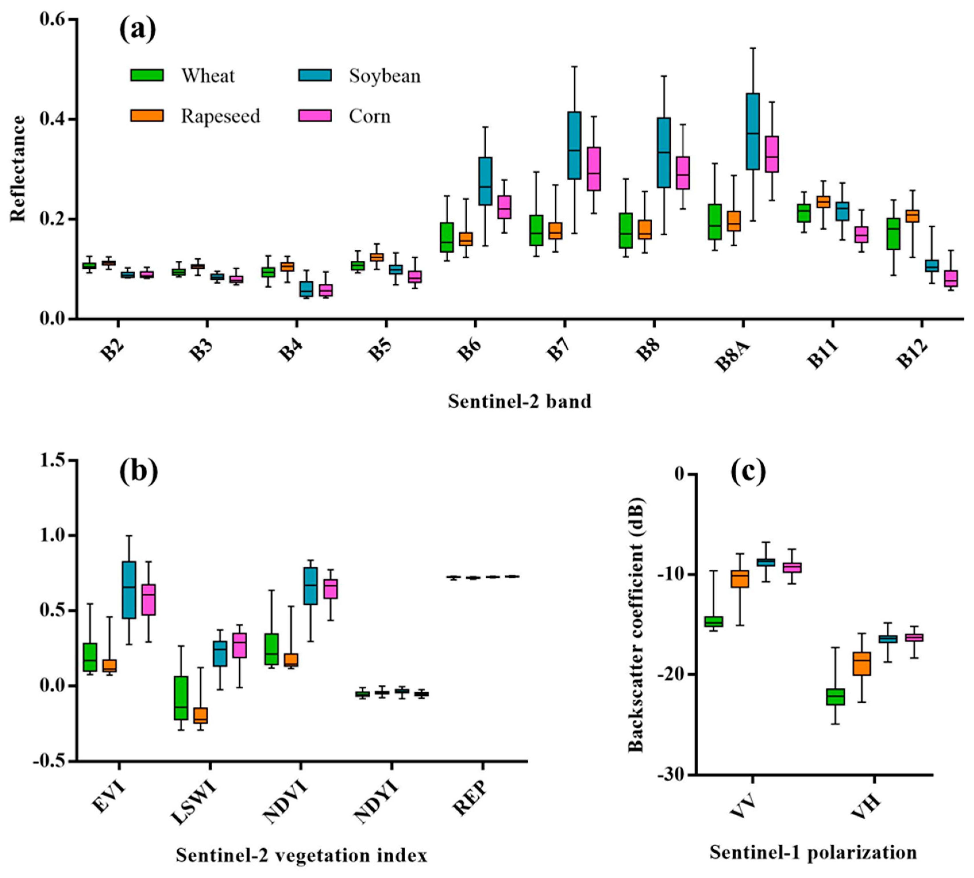
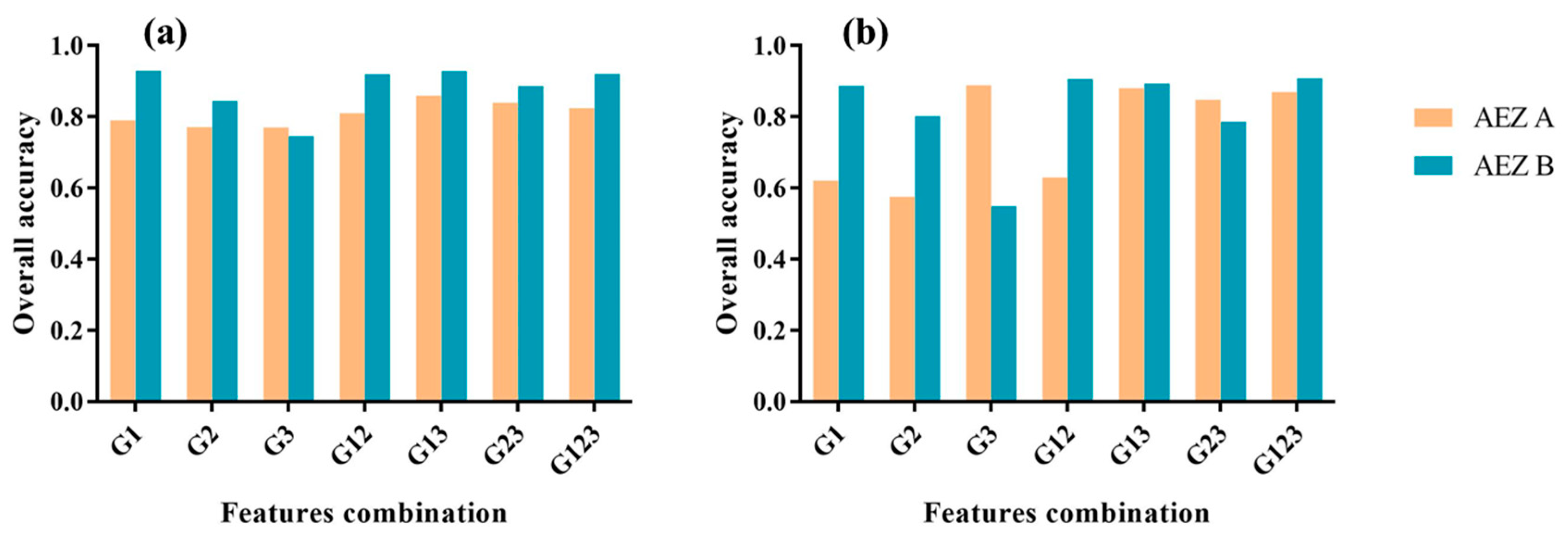
3.1. Sentinel Features in Crop Classification
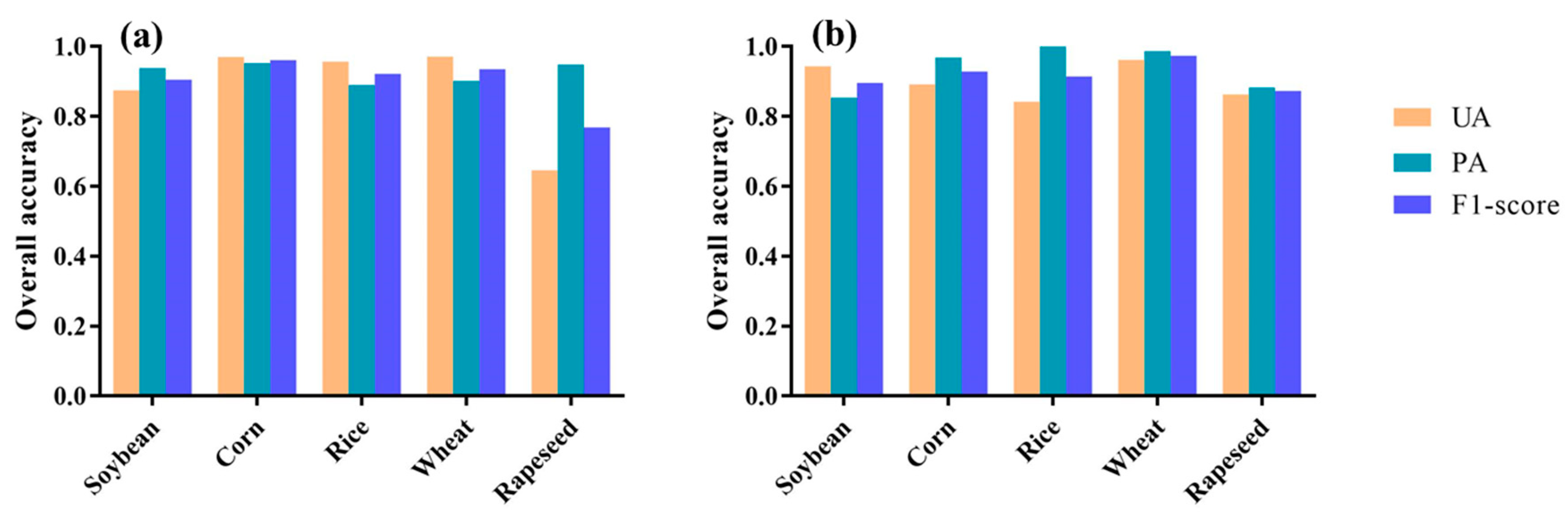
3.2. Classification Accuracy Assessment
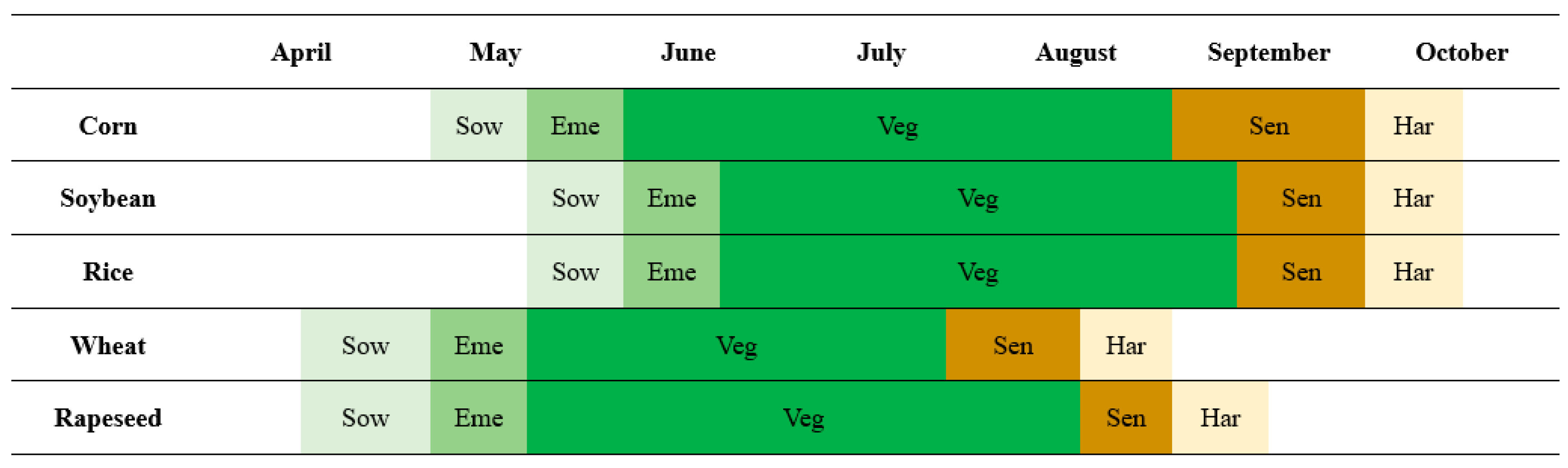
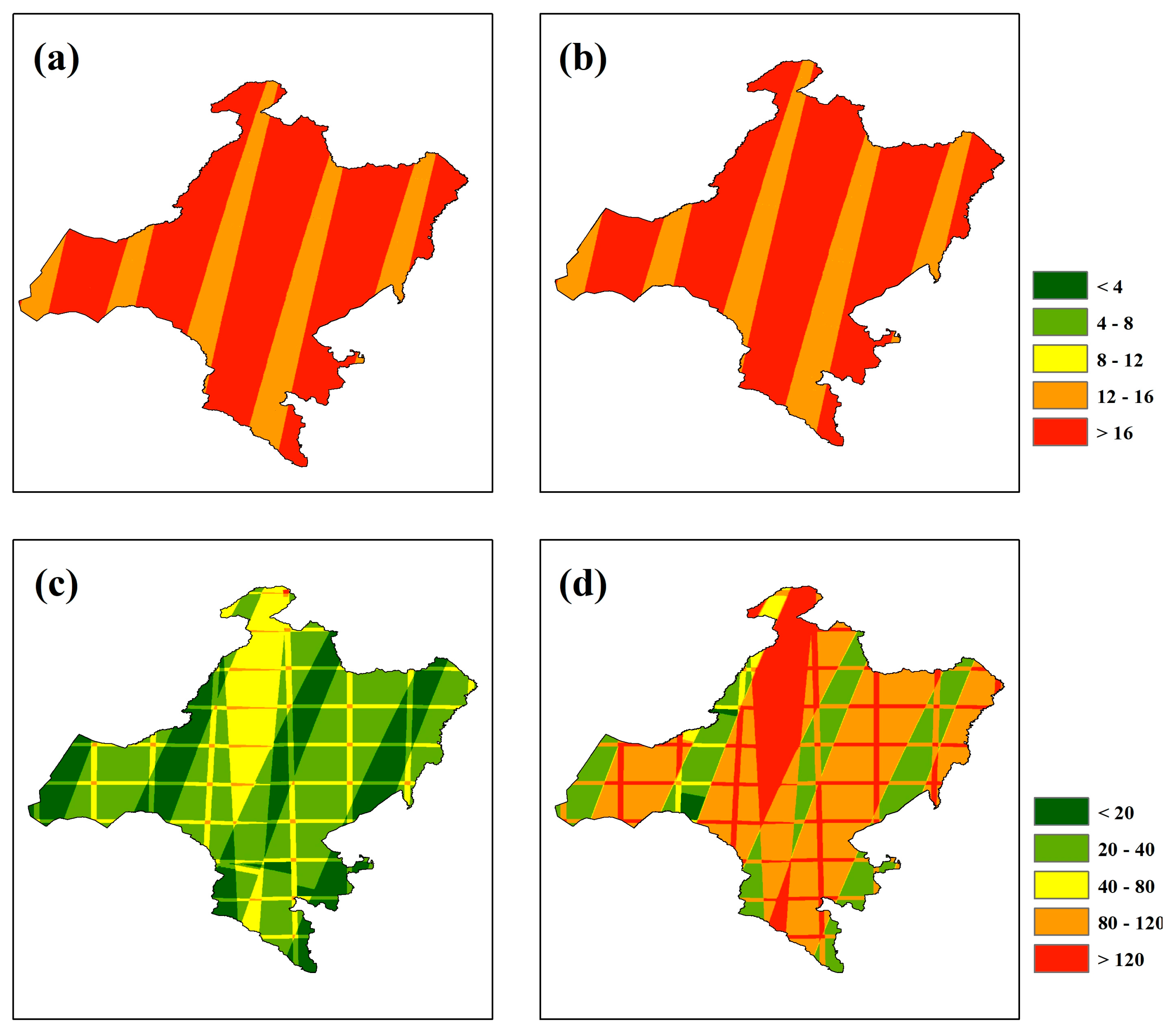
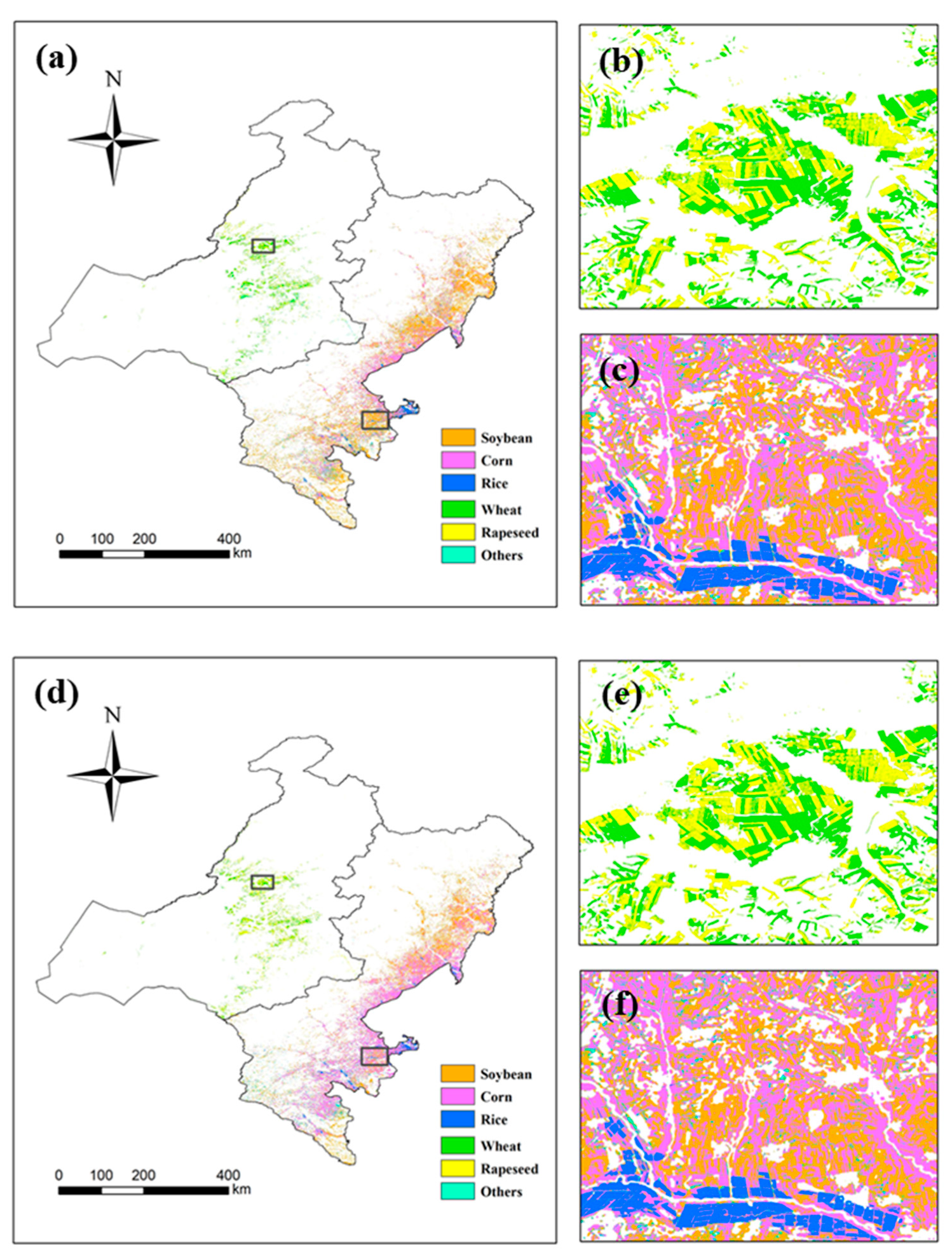
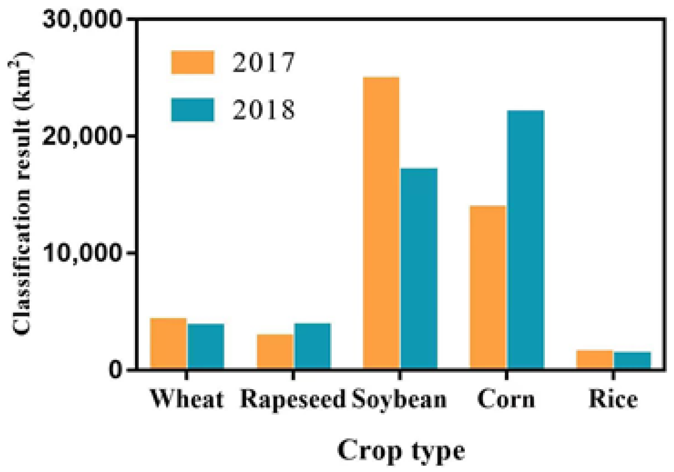
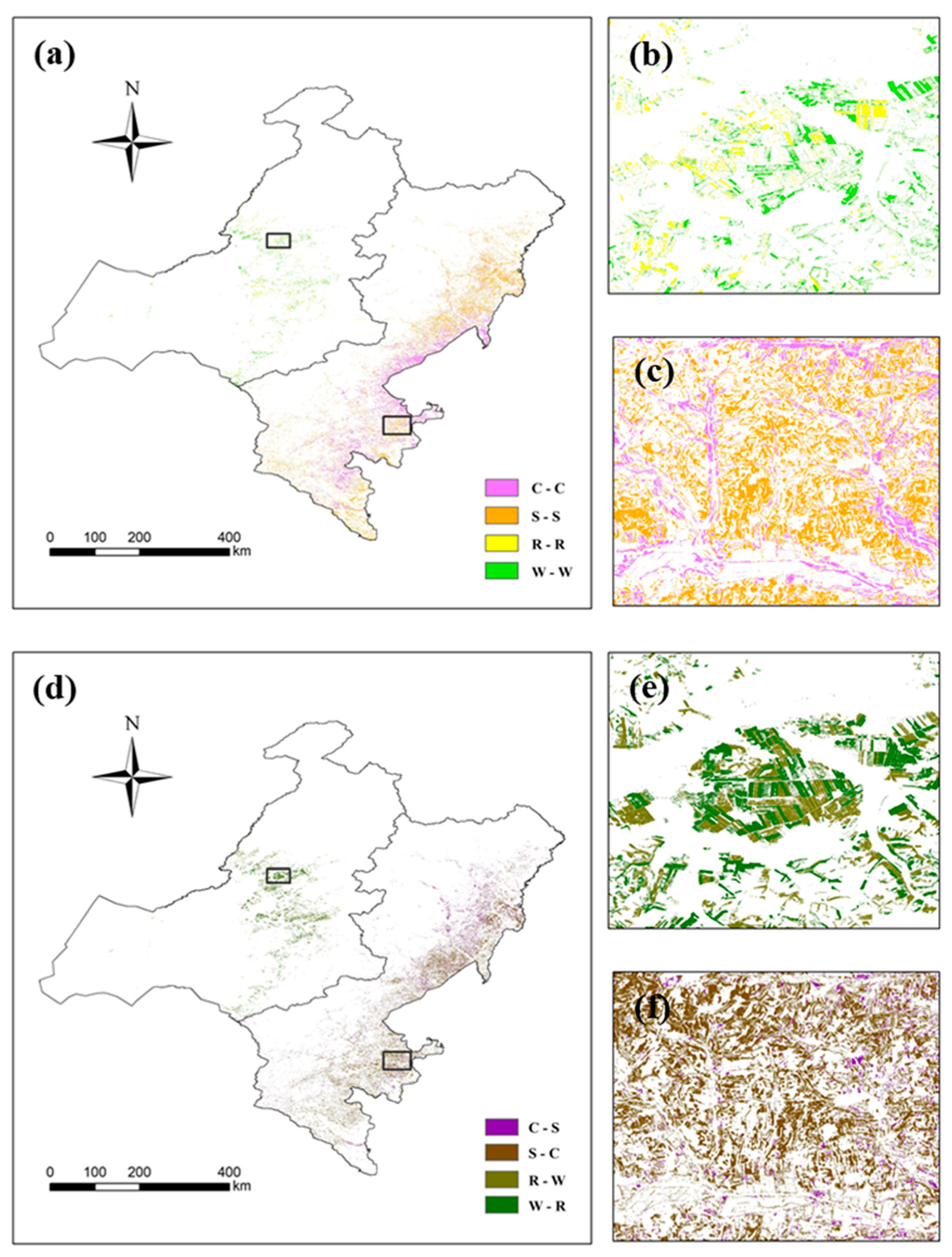
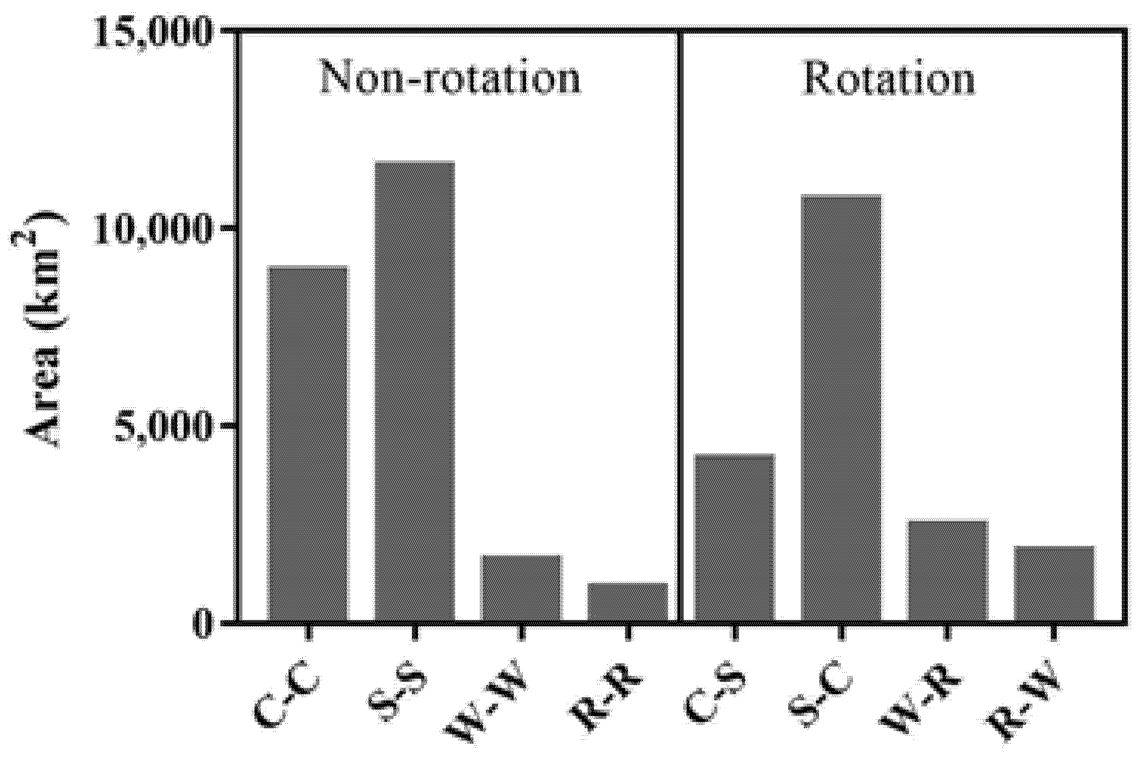
3.3. Crop Type Distribution and Rotation
4. Discussion
5. Conclusions
Author Contributions
Funding
Data Availability Statement
Acknowledgments
Conflicts of Interest
References
- Gong, P.; Wang, J.; Yu, L.; Zhao, Y.; Zhao, Y.; Liang, L.; Niu, Z.; Huang, X.; Fu, H.; Liu, S.; et al. Finer resolution observation and monitoring of global land cover: First mapping results with Landsat TM and ETM+ data. Int. J. Remote Sens. 2013, 34, 2607–2654. [Google Scholar] [CrossRef] [Green Version]
- Zhang, X.; Liu, L.; Chen, X.; Gao, Y.; Xie, S.; Mi, J. GLC_FCS30: Global land-cover product with fine classification system at 30 m using time-series Landsat imagery. Earth Syst. Sci. Data Discuss. 2020, 12, 1625–1648. [Google Scholar] [CrossRef]
- Bartholomé, E.; Belward, A.S. GLC2000: A new approach to global land cover mapping from Earth observation data. Int. J. Remote Sens. 2005, 26, 1959–1977. [Google Scholar] [CrossRef]
- Chen, J.; Chen, J.; Liao, A.; Cao, X.; Chen, L.; Chen, X.; He, C.; Han, G.; Peng, S.; Lu, M.; et al. Global land cover mapping at 30 m resolution: A POK-based operational approach. ISPRS J. Photogramm. Remote Sens. 2015, 103, 7–27. [Google Scholar] [CrossRef] [Green Version]
- Gong, P.; Liu, H.; Zhang, M.; Li, C.; Wang, J.; Huang, H.; Clinton, N.; Ji, L.; Li, W.; Bai, Y.; et al. Stable classification with limited sample: Transferring a 30-m resolution sample set collected in 2015 to mapping 10-m resolution global land cover in 2017. Sci. Bull. 2019, 64, 370–373. [Google Scholar] [CrossRef] [Green Version]
- Xiong, J.; Thenkabail, P.S.; Gumma, M.K.; Teluguntla, P.; Poehnelt, J.; Congalton, R.G.; Yadav, K.; Thau, D. Automated cropland mapping of continental Africa using Google Earth Engine cloud computing. ISPRS J. Photogramm. Remote Sens. 2017, 126, 225–244. [Google Scholar] [CrossRef] [Green Version]
- Dong, J.; Xiao, X.; Menarguez, M.A.; Zhang, G.; Qin, Y.; Thau, D.; Biradar, C.; Moore, B., III. Mapping paddy rice planting area in northeastern Asia with Landsat 8 images, phenology-based algorithm and Google Earth Engine. Remote Sens. Environ. 2016, 185, 142–154. [Google Scholar] [CrossRef] [Green Version]
- Cai, Y.; Guan, K.; Peng, J.; Wang, S.; Seifert, C.; Wardlow, B.; Li, Z. A high-performance and in-season classification system of field-level crop types using time-series Landsat data and a machine learning approach. Remote Sens. Environ. 2018, 210, 35–47. [Google Scholar] [CrossRef]
- Zhong, L.; Gong, P.; Biging, G.S. Efficient corn and soybean mapping with temporal extendability: A multi-year experiment using Landsat imagery. Remote Sens. Environ. 2014, 140, 1–13. [Google Scholar] [CrossRef]
- Qiu, B.; Li, W.; Tang, Z.; Chen, C.; Qi, W. Mapping paddy rice areas based on vegetation phenology and surface moisture conditions. Ecol. Indic. 2015, 56, 79–86. [Google Scholar] [CrossRef]
- Wardlow, B.D.; Egbert, S.L.; Kastens, J.H. Analysis of time-series MODIS 250 m vegetation index data for crop classification in the US Central Great Plains. Remote Sens. Environ. 2007, 108, 290–310. [Google Scholar] [CrossRef] [Green Version]
- Aksoy, S.; Yalniz, I.Z.; Tasdemir, K. Automatic Detection and Segmentation of Orchards Using Very High Resolution Imagery. IEEE Trans. Geosci. Remote Sens. 2012, 50, 3117–3131. [Google Scholar] [CrossRef]
- Jia, K.; Liang, S.; Zhang, N.; Wei, X.; Gu, X.; Zhao, X.; Yao, Y.; Xie, X. Land cover classification of finer resolution remote sensing data integrating temporal features from time series coarser resolution data. ISPRS J. Photogramm. Remote Sens. 2014, 93, 49–55. [Google Scholar] [CrossRef]
- Wardlow, B.D.; Egbert, S.L. Large-area crop mapping using time-series MODIS 250 m NDVI data: An assessment for the U.S. Central Great Plains. Remote Sens. Environ. 2008, 112, 1096–1116. [Google Scholar] [CrossRef]
- Fritz, S.; See, L.; McCallum, I.; You, L.; Bun, A.; Moltchanova, E.; Duerauer, M.; Albrecht, F.; Schill, C.; Perger, C.; et al. Mapping global cropland and field size. Glob. Chang. Biol. 2015, 21, 1980–1992. [Google Scholar] [CrossRef]
- Lobell, D.B.; Asner, G.P. Cropland distributions from temporal unmixing of MODIS data. Remote Sens. Environ. 2004, 93, 412–422. [Google Scholar] [CrossRef]
- Foerster, S.; Kaden, K.; Foerster, M.; Itzerott, S. Crop type mapping using spectral–temporal profiles and phenological information. Comput. Electron. Agric. 2012, 89, 30–40. [Google Scholar] [CrossRef] [Green Version]
- Zhang, H.; Du, H.; Zhang, C.; Zhang, L. An automated early-season method to map winter wheat using time-series Sentinel-2 data: A case study of Shandong, China. Comput. Electron. Agric. 2021, 182, 105962. [Google Scholar] [CrossRef]
- Dong, Q.; Chen, X.; Chen, J.; Zhang, C.; Liu, L.; Cao, X.; Zang, Y.; Zhu, X.; Cui, X. Mapping Winter Wheat in North China Using Sentinel 2A/B Data: A Method Based on Phenology-Time Weighted Dynamic Time Warping. Remote Sens. 2020, 12, 1274. [Google Scholar] [CrossRef] [Green Version]
- Waldner, F.; Diakogiannis, F.I. Deep learning on edge: Extracting field boundaries from satellite images with a convolutional neural network. Remote Sens. Environ. 2020, 245, 111741. [Google Scholar] [CrossRef]
- Mazarire, T.T.; Ratshiedana, P.E.; Nyamugama, A.; Adam, E.; Chirima, G. Exploring machine learning algorithms for mapping crop types in a heterogeneous agriculture landscape using Sentinel-2 data. A case study of Free State Province, South Africa. S. Afr. J. Geomat. 2020, 9, 333–347. [Google Scholar]
- Ibrahim, E.S.; Rufin, P.; Nill, L.; Kamali, B.; Nendel, C.; Hostert, P. Mapping Crop Types and Cropping Systems in Nigeria with Sentinel-2 Imagery. Remote Sens. 2021, 13, 3523. [Google Scholar] [CrossRef]
- Jin, Z.; Azzari, G.; You, C.; Di Tommaso, S.; Aston, S.; Burke, M.; Lobell, D.B. Smallholder maize area and yield mapping at national scales with Google Earth Engine. Remote Sens. Environ. 2019, 228, 115–128. [Google Scholar] [CrossRef]
- You, N.; Dong, J. Examining earliest identifiable timing of crops using all available Sentinel 1/2 imagery and Google Earth Engine. ISPRS J. Photogramm. Remote Sens. 2020, 161, 109–123. [Google Scholar] [CrossRef]
- Pott, L.P.; Amado, T.J.C.; Schwalbert, R.A.; Corassa, G.M.; Ciampitti, I.A. Satellite-based data fusion crop type classification and mapping in Rio Grande do Sul, Brazil. ISPRS J. Photogramm. Remote Sens. 2021, 176, 196–210. [Google Scholar] [CrossRef]
- Qiu, B.; Luo, Y.; Tang, Z.; Chen, C.; Lu, D.; Huang, H.; Chen, Y.; Chen, N.; Xu, W. Winter wheat mapping combining variations before and after estimated heading dates. ISPRS J. Photogramm. Remote Sens. 2017, 123, 35–46. [Google Scholar] [CrossRef]
- Tian, H.; Huang, N.; Niu, Z.; Qin, Y.; Pei, J.; Wang, J. Mapping Winter Crops in China with Multi-Source Satellite Imagery and Phenology-Based Algorithm. Remote Sens. 2019, 11, 820. [Google Scholar] [CrossRef] [Green Version]
- Xu, X.; Ji, X.; Jiang, J.; Yao, X.; Tian, Y.; Zhu, Y.; Cao, W.; Cao, Q.; Yang, H.; Shi, Z.; et al. Evaluation of One-Class Support Vector Classification for Mapping the Paddy Rice Planting Area in Jiangsu Province of China from Landsat 8 OLI Imagery. Remote Sens. 2018, 10, 546. [Google Scholar] [CrossRef] [Green Version]
- Zhang, X.; Yang, G.; Xu, X.; Yao, X.; Zheng, H.; Zhu, Y.; Cao, W.; Cheng, T. An assessment of Planet satellite imagery for county-wide mapping of rice planting areas in Jiangsu Province, China with one-class classification approaches. Int. J. Remote Sens. 2021, 42, 7610–7635. [Google Scholar] [CrossRef]
- Dong, J.; Fu, Y.; Wang, J.; Tian, H.; Fu, S.; Niu, Z.; Han, W.; Zheng, Y.; Huang, J.; Yuan, W. Early-season mapping of winter wheat in China based on Landsat and Sentinel images. Earth Syst. Sci. Data 2020, 12, 3081–3095. [Google Scholar] [CrossRef]
- Zhong, L.; Hu, L.; Zhou, H. Deep learning based multi-temporal crop classification. Remote Sens. Environ. 2019, 221, 430–443. [Google Scholar] [CrossRef]
- Egorov, A.V.; Hansen, M.C.; Roy, D.P.; Kommareddy, A.; Potapov, P.V. Image interpretation-guided supervised classification using nested segmentation. Remote Sens. Environ. 2015, 165, 135–147. [Google Scholar] [CrossRef] [Green Version]
- Sharma, R.; Ghosh, A.; Joshi, P.K. Decision tree approach for classification of remotely sensed satellite data using open source support. J. Earth Syst. Sci. 2013, 122, 1237–1247. [Google Scholar] [CrossRef] [Green Version]
- Waldner, F.; Canto, G.S.; Defourny, P. Automated annual cropland mapping using knowledge-based temporal features. ISPRS J. Photogramm. Remote Sens. 2015, 110, 1–13. [Google Scholar] [CrossRef]
- Kluger, D.M.; Wang, S.; Lobell, D.B. Two shifts for crop mapping: Leveraging aggregate crop statistics to improve satellite-based maps in new regions. Remote Sens. Environ. 2021, 262, 112488. [Google Scholar] [CrossRef]
- Song, Q.; Hu, Q.; Zhou, Q.; Hovis, C.; Xiang, M.; Tang, H.; Wu, W. In-Season Crop Mapping with GF-1/WFV Data by Combining Object-Based Image Analysis and Random Forest. Remote Sens. 2017, 9, 1184. [Google Scholar] [CrossRef] [Green Version]
- He, Y.; Wang, C.; Chen, F.; Jia, H.; Liang, D.; Yang, A. Feature Comparison and Optimization for 30-M Winter Wheat Mapping Based on Landsat-8 and Sentinel-2 Data Using Random Forest Algorithm. Remote Sens. 2019, 11, 535. [Google Scholar] [CrossRef] [Green Version]
- Kpienbaareh, D.; Sun, X.; Wang, J.; Luginaah, I.; Bezner Kerr, R.; Lupafya, E.; Dakishoni, L. Crop Type and Land Cover Mapping in Northern Malawi Using the Integration of Sentinel-1, Sentinel-2, and PlanetScope Satellite Data. Remote Sens. 2021, 13, 700. [Google Scholar] [CrossRef]
- Palchowdhuri, Y.; Valcarce-Diñeiro, R.; King, P.; Sanabria-Soto, M. Classification of multi-temporal spectral indices for crop type mapping: A case study in Coalville, UK. J. Agric. Sci. 2018, 156, 24–36. [Google Scholar] [CrossRef]
- Gorelick, N.; Hancher, M.; Dixon, M.; Ilyushchenko, S.; Thau, D.; Moore, R. Google Earth Engine: Planetary-scale geospatial analysis for everyone. Remote Sens. Environ. 2017, 202, 18–27. [Google Scholar] [CrossRef]
- Teluguntla, P.; Thenkabail, P.S.; Oliphant, A.; Xiong, J.; Gumma, M.K.; Congalton, R.G.; Yadav, K.; Huete, A. A 30-m landsat-derived cropland extent product of Australia and China using random forest machine learning algorithm on Google Earth Engine cloud computing platform. ISPRS J. Photogramm. Remote Sens. 2018, 144, 325–340. [Google Scholar] [CrossRef]
- Phalke, A.R.; Özdoğan, M.; Thenkabail, P.S.; Erickson, T.; Gorelick, N.; Yadav, K.; Congalton, R.G. Mapping croplands of Europe, Middle East, Russia, and Central Asia using Landsat, Random Forest, and Google Earth Engine. ISPRS J. Photogramm. Remote Sens. 2020, 167, 104–122. [Google Scholar] [CrossRef]
- Oliphant, A.J.; Thenkabail, P.S.; Teluguntla, P.; Xiong, J.; Gumma, M.K.; Congalton, R.G.; Yadav, K. Mapping cropland extent of Southeast and Northeast Asia using multi-year time-series Landsat 30-m data using a random forest classifier on the Google Earth Engine Cloud. Int. J. Appl. Earth Obs. Geoinf. 2019, 81, 110–124. [Google Scholar] [CrossRef]
- Liu, L.; Xiao, X.; Qin, Y.; Wang, J.; Xu, X.; Hu, Y.; Qiao, Z. Mapping cropping intensity in China using time series Landsat and Sentinel-2 images and Google Earth Engine. Remote Sens. Environ. 2020, 239, 111624. [Google Scholar] [CrossRef]
- Zhang, M.; Wu, B.; Zeng, H.; He, G.; Liu, C.; Tao, S.; Zhang, Q.; Nabil, M.; Tian, F.; Bofana, J.; et al. GCI30: A global dataset of 30-m cropping intensity using multisource remote sensing imagery. Earth Syst. Sci. Data Discuss. 2021, 13, 4799–4817. [Google Scholar] [CrossRef]
- Ni, R.; Tian, J.; Li, X.; Yin, D.; Li, J.; Gong, H.; Zhang, J.; Zhu, L.; Wu, D. An enhanced pixel-based phenological feature for accurate paddy rice mapping with Sentinel-2 imagery in Google Earth Engine. ISPRS J. Photogramm. Remote Sens. 2021, 178, 282–296. [Google Scholar] [CrossRef]
- Ge, S.; Zhang, J.; Pan, Y.; Yang, Z.; Zhu, S. Transferable deep learning model based on the phenological matching principle for mapping crop extent. Int. J. Appl. Earth Obs. Geoinf. 2021, 102, 102451. [Google Scholar] [CrossRef]
- Duan, Q.; Tan, M.; Guo, Y.; Wang, X.; Xin, L. Understanding the Spatial Distribution of Urban Forests in China Using Sentinel-2 Images with Google Earth Engine. Forests 2019, 10, 729. [Google Scholar] [CrossRef] [Green Version]
- Jia, M.; Wang, Z.; Mao, D.; Ren, C.; Wang, C.; Wang, Y. Rapid, robust, and automated mapping of tidal flats in China using time series Sentinel-2 images and Google Earth Engine. Remote Sens. Environ. 2021, 255, 112285. [Google Scholar] [CrossRef]
- Liu, W.; Wang, J.; Luo, J.; Wu, Z.; Chen, J.; Zhou, Y.; Sun, Y.; Shen, Z.; Xu, N.; Yang, Y. Farmland Parcel Mapping in Mountain Areas Using Time-Series SAR Data and VHR Optical Images. Remote Sens. 2020, 12, 3733. [Google Scholar] [CrossRef]
- Burke, M.; Lobell, D.B. Satellite-based assessment of yield variation and its determinants in smallholder African systems. Proc. Natl. Acad. Sci. USA 2017, 114, 2189–2194. [Google Scholar] [CrossRef] [PubMed] [Green Version]
- Wang, Y.-C.; Feng, C.-C.; Vu Duc, H. Integrating Multi-Sensor Remote Sensing Data for Land Use/Cover Mapping in a Tropical Mountainous Area in Northern Thailand. Geogr. Res. 2012, 50, 320–331. [Google Scholar] [CrossRef]
- Boryan, C.; Yang, Z.; Mueller, R.; Craig, M. Monitoring US agriculture: The US Department of Agriculture, National Agricultural Statistics Service, Cropland Data Layer Program. Geocarto Int. 2011, 26, 341–358. [Google Scholar] [CrossRef]
- Fisette, T.; Davidson, A.; Daneshfar, B.; Rollin, P.; Aly, Z.; Campbell, L. Annual Space-Based Crop Inventory for Canada: 2009–2014. In Proceedings of the IEEE Geoscience and Remote Sensing Symposium, Quebec, QC, Canada, 13–18 July 2014; pp. 5095–5098. [Google Scholar]
- Conrad, C.; Lamers, J.P.A.; Ibragimov, N.; Löw, F.; Martius, C. Analysing irrigated crop rotation patterns in arid Uzbekistan by the means of remote sensing: A case study on post-Soviet agricultural land use. J. Arid Environ. 2016, 124, 150–159. [Google Scholar] [CrossRef]
- Lesiv, M.; Laso Bayas, J.C.; See, L.; Duerauer, M.; Dahlia, D.; Durando, N.; Hazarika, R.; Kumar Sahariah, P.; Vakolyuk, M.; Blyshchyk, V.; et al. Estimating the global distribution of field size using crowdsourcing. Glob. Chang. Biol. 2018, 25, 174–186. [Google Scholar] [CrossRef]
- You, N.; Dong, J.; Huang, J.; Du, G.; Zhang, G.; He, Y.; Yang, T.; Di, Y.; Xiao, X. The 10-m crop type maps in Northeast China during 2017–2019. Sci. Data 2021, 8, 41. [Google Scholar] [CrossRef]
- Yu, L.; Wulantuya; Li, J.; Yu, W.; Dun, H. Multi-source remote sensing data feature optimization for different crop extraction in Daxing’Anling along the foothills. J. North Agric. 2020, 48, 119–128, (In Chinese with English Abstract). [Google Scholar]
- Yu, L.; Wulantuya; Wulan; Bao, J. Study on the main crop identification method based on SAR-C in the west of Great Khingan Mountains. J. North. Agric. 2017, 45, 108–113, (In Chinese with English Abstract). [Google Scholar]
- Yang, L.; Wang, L.; Huang, J.; Mansaray, L.R.; Mijiti, R. Monitoring policy-driven crop area adjustments in northeast China using Landsat-8 imagery. Int. J. Appl. Earth Obs. Geoinf. 2019, 82, 101892. [Google Scholar] [CrossRef]
- Liu, S.; Zhang, P.; Liu, W.; He, X. Key Factors Affecting Farmers’ Choice of Corn Reduction under the China’s New Agriculture Policy in the ‘Liandaowan’ Areas, Northeast China. Chin. Geogr. Sci. 2019, 29, 1039–1051. [Google Scholar] [CrossRef] [Green Version]
- Ghorbanian, A.; Kakooei, M.; Amani, M.; Mahdavi, S.; Mohammadzadeh, A.; Hasanlou, M. Improved land cover map of Iran using Sentinel imagery within Google Earth Engine and a novel automatic workflow for land cover classification using migrated training samples. ISPRS J. Photogramm. Remote Sens. 2020, 167, 276–288. [Google Scholar] [CrossRef]
- Yang, G.; Yu, W.; Yao, X.; Zheng, H.; Cao, Q.; Zhu, Y.; Cao, W.; Cheng, T. AGTOC: A novel approach to winter wheat mapping by automatic generation of training samples and one-class classification on Google Earth Engine. Int. J. Appl. Earth Obs. Geoinf. 2021, 102, 102446. [Google Scholar] [CrossRef]
- Song, C.; Woodcock, C.E.; Seto, K.C.; Lenney, M.P.; Macomber, S.A. Classification and change detection using Landsat TM data: When and how to correct atmospheric effects? Remote Sens. Environ. 2001, 75, 230–244. [Google Scholar] [CrossRef]
- Huete, A.; Didan, K.; Miura, T.; Rodriguez, E.P.; Gao, X.; Ferreira, L.G. Overview of the radiometric and biophysical performance of the MODIS vegetation indices. Remote Sens. Environ. 2002, 83, 195–213. [Google Scholar] [CrossRef]
- Bocai, G. NDWI—A normalized difference water index for remote sensing of vegetation liquid water from space. Remote Sens. Environ. 1996, 58, 257–266. [Google Scholar]
- Rouse, J.; Haas, R.; Schell, J.; Deering, D. Monitoring Vegetation Systems in the Great Plains with ERTS. NASA Spec. Publ. 1974, 351, 309. [Google Scholar]
- Sulik, J.J.; Long, D.S. Spectral considerations for modeling yield of canola. Remote Sens. Environ. 2016, 184, 161–174. [Google Scholar] [CrossRef] [Green Version]
- Guyot, G.; Frederic, B.; Jacquemoud, S. Imaging spectroscopy for vegetation studies. Imaging Spectrosc. 1992, 2, 145–165. [Google Scholar]
- Friedl, M.A.; Brodley, C.E.; Strahler, A.H. Maximizing land cover classification accuracies produced by decision trees at continental to global scales. IEEE Trans. Geosci. Remote Sens. 1999, 37, 969–977. [Google Scholar] [CrossRef]
- Huang, H.; Wang, J.; Liu, C.; Liang, L.; Li, C.; Gong, P. The migration of training samples towards dynamic global land cover mapping. ISPRS J. Photogramm. Remote Sens. 2020, 161, 27–36. [Google Scholar] [CrossRef]
- Zhong, L.; Hu, L.; Yu, L.; Gong, P.; Biging, G.S. Automated mapping of soybean and corn using phenology. ISPRS J. Photogramm. Remote Sens. 2016, 119, 151–164. [Google Scholar] [CrossRef] [Green Version]
- Hao, P.; Di, L.; Zhang, C.; Guo, L. Transfer Learning for Crop classification with Cropland Data Layer data (CDL) as training samples. Sci. Total Environ. 2020, 733, 138869. [Google Scholar] [CrossRef] [PubMed]
- Maskell, G.; Chemura, A.; Nguyen, H.; Gornott, C.; Mondal, P. Integration of Sentinel optical and radar data for mapping smallholder coffee production systems in Vietnam. Remote Sens. Environ. 2021, 266, 112709. [Google Scholar] [CrossRef]
- Prins, A.J.; Van Niekerk, A. Crop type mapping using LiDAR, Sentinel-2 and aerial imagery with machine learning algorithms. Geo-Spat. Inf. Sci. 2021, 24, 215–227. [Google Scholar] [CrossRef]
- Delrue, J.; Bydekerke, L.; Eerens, H.; Gilliams, S.; Piccard, I.; Swinnen, E. Crop mapping in countries with small-scale farming: A case study for West Shewa, Ethiopia. Int. J. Remote Sens. 2012, 34, 2566–2582. [Google Scholar] [CrossRef]
- Chen, B.; Jin, Y.; Brown, P. An enhanced bloom index for quantifying floral phenology using multi-scale remote sensing observations. ISPRS J. Photogramm. Remote Sens. 2019, 156, 108–120. [Google Scholar] [CrossRef]
- D’Andrimont, R.; Taymans, M.; Lemoine, G.; Ceglar, A.; Yordanov, M.; van der Velde, M. Detecting flowering phenology in oil seed rape parcels with Sentinel-1 and -2 time series. Remote Sens. Environ. 2020, 239, 111660. [Google Scholar] [CrossRef]
- Mercier, A.; Betbeder, J.; Baudry, J.; Le Roux, V.; Spicher, F.; Lacoux, J.; Roger, D.; Hubert-Moy, L. Evaluation of Sentinel-1 & 2 time series for predicting wheat and rapeseed phenological stages. ISPRS J. Photogramm. Remote Sens. 2020, 163, 231–256. [Google Scholar]
- Inoue, Y.; Sakaiya, E.; Wang, C.Z. Capability of C-band backscattering coefficients from high-resolution satellite SAR sensors to assess biophysical variables in paddy rice. Remote Sens. Environ. 2014, 140, 257–266. [Google Scholar] [CrossRef]
- Mattia, F.; Le Toan, T.; Picard, G.; Posa, F.I.; D’Alessio, A.; Notarnicola, C.; Gatti, A.M.; Rinaldi, M.; Satalino, G.; Pasquariello, G. Multitemporal C-band radar measurements on wheat fields. IEEE Trans. Geosci. Remote Sens. 2003, 41, 1551–1560. [Google Scholar] [CrossRef]
- Song, X.-P.; Potapov, P.V.; Krylov, A.; King, L.; Di Bella, C.M.; Hudson, A.; Khan, A.; Adusei, B.; Stehman, S.V.; Hansen, M.C. National-scale soybean mapping and area estimation in the United States using medium resolution satellite imagery and field survey. Remote Sens. Environ. 2017, 190, 383–395. [Google Scholar] [CrossRef]
- Defourny, P.; Bontemps, S.; Bellemans, N.; Cara, C.; Dedieu, G.; Guzzonato, E.; Hagolle, O.; Inglada, J.; Nicola, L.; Rabaute, T.; et al. Near real-time agriculture monitoring at national scale at parcel resolution: Performance assessment of the Sen2-Agri automated system in various cropping systems around the world. Remote Sens. Environ. 2019, 221, 551–568. [Google Scholar] [CrossRef]
- Ozdogan, M.; Woodcock, C.E. Resolution dependent errors in remote sensing of cultivated areas. Remote Sens. Environ. 2006, 103, 203–217. [Google Scholar] [CrossRef]
- Su, T.; Zhang, S. Object-based crop classification in Hetao plain using random forest. Earth Sci. Inf. 2021, 14, 119–131. [Google Scholar] [CrossRef]
- Tang, Z.; Wang, H.; Li, X.; Li, X.; Cai, W.; Han, C. An Object-Based Approach for Mapping Crop Coverage Using Multiscale Weighted and Machine Learning Methods. IEEE J. Sel. Top. Appl. Earth Obs. Remote Sens. 2020, 13, 1700–1713. [Google Scholar] [CrossRef]


| Total Observation of S1 | Total Observation of S2 | Good Observation of S2 | |
|---|---|---|---|
| 2017 | 407 | 1492 | 505 |
| 2018 | 398 | 3777 | 1476 |
| VIs | Full Name | Formula | Reference |
|---|---|---|---|
| EVI | Enhanced Vegetation Index | 2.5 × (NIR − Red)/(NIR + 6 × Red − 7.5 × Blue + 1) | [65] |
| LSWI | Land Surface Water Index | (NIR − SWIR1)/(NIR + SWIR1) | [66] |
| NDVI | Normalized Difference Vegetation Index | (NIR − Red)/(NIR + Red) | [67] |
| NDYI | Normalized Difference Yellow Index | (Green − Blue)/(Green + Blue) | [68] |
| REP | Red Edge Position | 705 + 35 × (0.5 × (RE3 + Red) − RE1)/(RE2 − RE1) | [69] |
| Crop Type | 2017 | 2018 |
|---|---|---|
| Soybean | 60 | 57 |
| Corn | 63 | 63 |
| Rice | 31 | 29 |
| Wheat | 55 | 55 |
| Rapeseed | 52 | 60 |
| Others | 27 | 25 |
| Total | 288 | 289 |
| Group | Features |
|---|---|
| G1 | B2, B3, B4, B5, B6, B7, B8, B8A, B11, B12 |
| G2 | EVI, LSWI, NDVI, NDYI, REP |
| G3 | VV, VH |
| G12 | G1 + G2 |
| G13 | G1 + G3 |
| G23 | G2 + G3 |
| G123 | G1 + G2 + G3 |
Publisher’s Note: MDPI stays neutral with regard to jurisdictional claims in published maps and institutional affiliations. |
© 2022 by the authors. Licensee MDPI, Basel, Switzerland. This article is an open access article distributed under the terms and conditions of the Creative Commons Attribution (CC BY) license (https://creativecommons.org/licenses/by/4.0/).
Share and Cite
Ren, T.; Xu, H.; Cai, X.; Yu, S.; Qi, J. Smallholder Crop Type Mapping and Rotation Monitoring in Mountainous Areas with Sentinel-1/2 Imagery. Remote Sens. 2022, 14, 566. https://doi.org/10.3390/rs14030566
Ren T, Xu H, Cai X, Yu S, Qi J. Smallholder Crop Type Mapping and Rotation Monitoring in Mountainous Areas with Sentinel-1/2 Imagery. Remote Sensing. 2022; 14(3):566. https://doi.org/10.3390/rs14030566
Chicago/Turabian StyleRen, Tingting, Hongtao Xu, Xiumin Cai, Shengnan Yu, and Jiaguo Qi. 2022. "Smallholder Crop Type Mapping and Rotation Monitoring in Mountainous Areas with Sentinel-1/2 Imagery" Remote Sensing 14, no. 3: 566. https://doi.org/10.3390/rs14030566