Air-Ground Multi-Source Image Matching Based on High-Precision Reference Image

Abstract

Robustness of aerial-ground multi-source image matching is closely related to the quality of the ground reference image. To explore the influence of reference images on the performance of air-ground multi-source image matching, we focused on the impact of the control point projection accuracy and tie point accuracy on bundle adjustment results for generating digital orthophoto images by using the Structure from Motion algorithm and Monte Carlo analysis. Additionally, we developed a method to learn local deep features in natural environments based on fine-tuning the pre-trained ResNet50 model and used the method to match multi-scale, multi-seasonal, and multi-viewpoint air-ground multi-source images. The results show that the proposed method could yield a relatively even distribution of feature corresponding points under different conditions, seasons, viewpoints, illuminations. Compared with state-of-the-art hand-crafted computer vision and deep learning matching methods, the proposed method demonstrated more efficient and robust matching performance that could be applied to a variety of unmanned aerial vehicle self- and target-positioning applications in GPS-denied areas.

1. Introduction

Air-ground multi-source image matching is the process of finding corresponding points between two images taken of the same scene but under different sensors, viewpoint, time, and weather conditions [1]. Fast and accurate image matching is particularly important for unmanned aerial vehicles (UAVs) to allow them to perform tasks such as image registration, battlefield reconnaissance, and environmental monitoring [2,3]. Air-ground image matching aims to find robust features of images acquired by UAVs that are consistent with a previous reference image. The key to successful matching is an appropriate matching strategy, making use of all available and explicit knowledge concerning the sensor model, network structure, and image content. In the multi-source UAV image acquisition phase, differences in resolution, viewpoint, scale, sensor model, and illumination conditions will lead to feature confusion and object occlusion problems in the images. Differences in the internal parameters of the camera can also cause differences in image quality. Additionally, images collected at different times may show changes to the number or presence of objects. These factors make image matching more difficult.

To represent the content of the image accurately, many feature extraction methods have been designed. Conventional hand-crafted computer vision matching methods, such as scale-invariant feature transform (SIFT) [4], speeded up robust features (SURF) [5], oriented FAST and rotated BRIEF (ORB) [6], and AKAZE [7], are widely used to solve matching tasks by computing the correspondences between two images. The point feature matching method based on feature descriptors and geometric constraints is the most widespread alternative. This typical method uses the similarity constraints of the feature descriptor set to calculate initial corresponding points and then eliminates mismatches using geometric constraints between feature corresponding points set. The Euclidean distance or Hamming distance of feature descriptors is used to measure similarity, which is the basis of feature matching. However, the low-level information cannot effectively handle image transformations such as rotations and illumination changes. When directly applying these algorithms to multi-source image matching, it becomes difficult to obtain the desired matching results [8]. Feature detection, feature description, and appropriate matching strategies can be used to obtain a wide range of robust matching results. The complete process of image feature matching involves three stages, each with a different emphasis. The process includes feature detection, feature description, and feature matching, which are all popular research topics. The feature matching stage requires an appropriate matching strategy to generate correct and uniformly distributed information feature correspondences. Improvements to the performance of feature matching have predominantly been achieved by researchers through improving the feature extraction operator [9,10], improving the feature descriptor [11], and improving the matching strategy [12]. However, they are still not robust for large-scale multi-view and multi-temporal air-ground image matching.

In recent years, convolutional neural networks (CNN) have provided more powerful feature representations for various types of image feature recognition and matching tasks [13]. The main difference between a deep feature and a visual feature is that image deep features are learned automatically from large-scale datasets rather than being developed manually. Based on the characteristics of CNNs, the output layers of the different networks have different levels of image visual representation [14,15]. In general, the signals of the input layer are highly versatile, and the signals of the output layer are easily fitted using specific training data. Convolutional layer features have stronger associated image discrimination and more detailed description capabilities than fully connected layer features. Since deep features are a type of feature representation based on data-driven learning, CNN models with strong feature representation and generalization capabilities often require a large training dataset [16,17]. As the CNN layers continue to deepen, the model’s expression capabilities are enhanced. However, collecting sufficient training data is tedious and time-consuming, which may even be considered unrealistic in many scenarios, especially in unknown areas which are not easily accessible. Research on the processing of image features to improve CNN expression capabilities when training data are insufficient is the focus of current research [18]. Oquab et al. [19] found that transfer learning between different learning tasks can be achieved by fine-tuning pre-trained models to yield state-of-the-art results on challenging benchmark datasets of much smaller sizes. Guo et al. [20] proposed an adaptive fine-tuning algorithm that specializes in the fine-tuning strategy for each training example of the target dataset. Comparison with other state-of-the-art fine-tuning strategies shows its superior performance. Sara et al. [21] proposed a fine-tuning model ensemble strategy that could be used to optimize deep learning model parameter settings and save more computational resources. Nima et al. [22] demonstrated that a pre-trained CNN with adequate fine-tuning performed as well as a CNN trained from scratch. Fine-tuned CNNs were more robust to the size of the training datasets than CNNs trained from scratch. They also found that shallow tuning nor deep tuning was the optimal choice for a particular application. Maggiori et al. [23] fine-tuned a network by using a small part of a carefully labeled image to output more accurate classifications. After proper fine-tuning, low-level features tended to be preserved from one dataset to another, while the higher layer parameters were updated to adapt the network to the new problem [24]. Since our study goal was to obtain UAV images of target areas by simulation in unknown environments, the training dataset would typically be small. The existing studies mostly used the matching of UAV’s look-down images with reference images [25,26], while the study on the matching of large-inclination and multi-view UAV images with reference images is relatively rare. The focus of this study was the development of a method of using the pre-trained model to effectively represent the image deep features and thus improve the robustness of large-scale and multi-temporal image matching.

For the robust matching of air-ground multi-source images, the key problem is how to design better image matching methods with superior performance in accuracy, robustness, and efficiency [27]. In addition, reference image accuracy solution is an essential part of aerial triangulation. To fully appreciate the impact of digital orthophoto map (DOM) and digital surface model (DSM) accuracy on image matching, we first provided a detailed description of problems related to quality when using UAV images to construct reference images based on the structure from motion (SFM) algorithm. The local deep features are extracted from multi-source UAV sequence images to match the deep features of the reference image. The process involves two main stages:

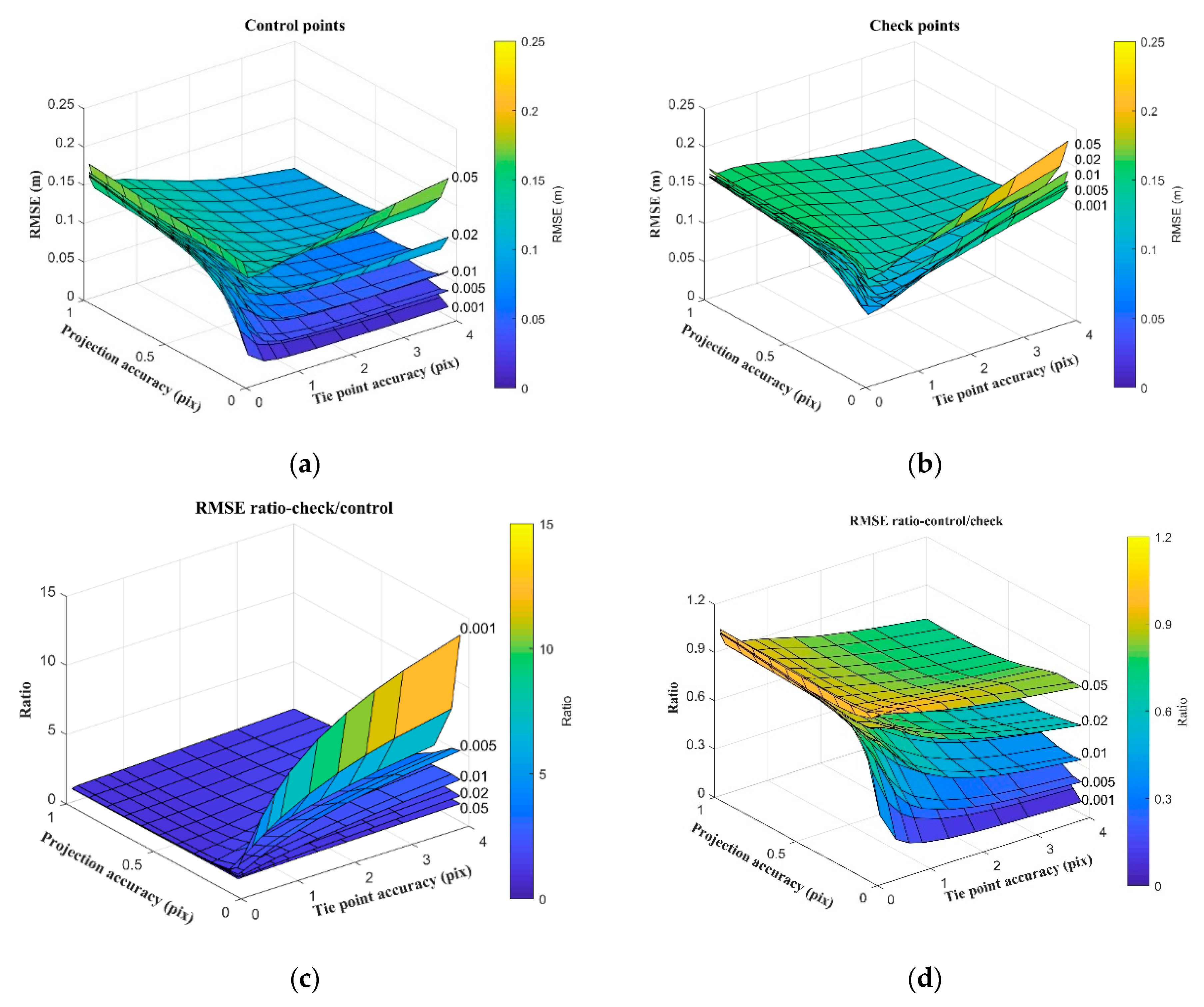
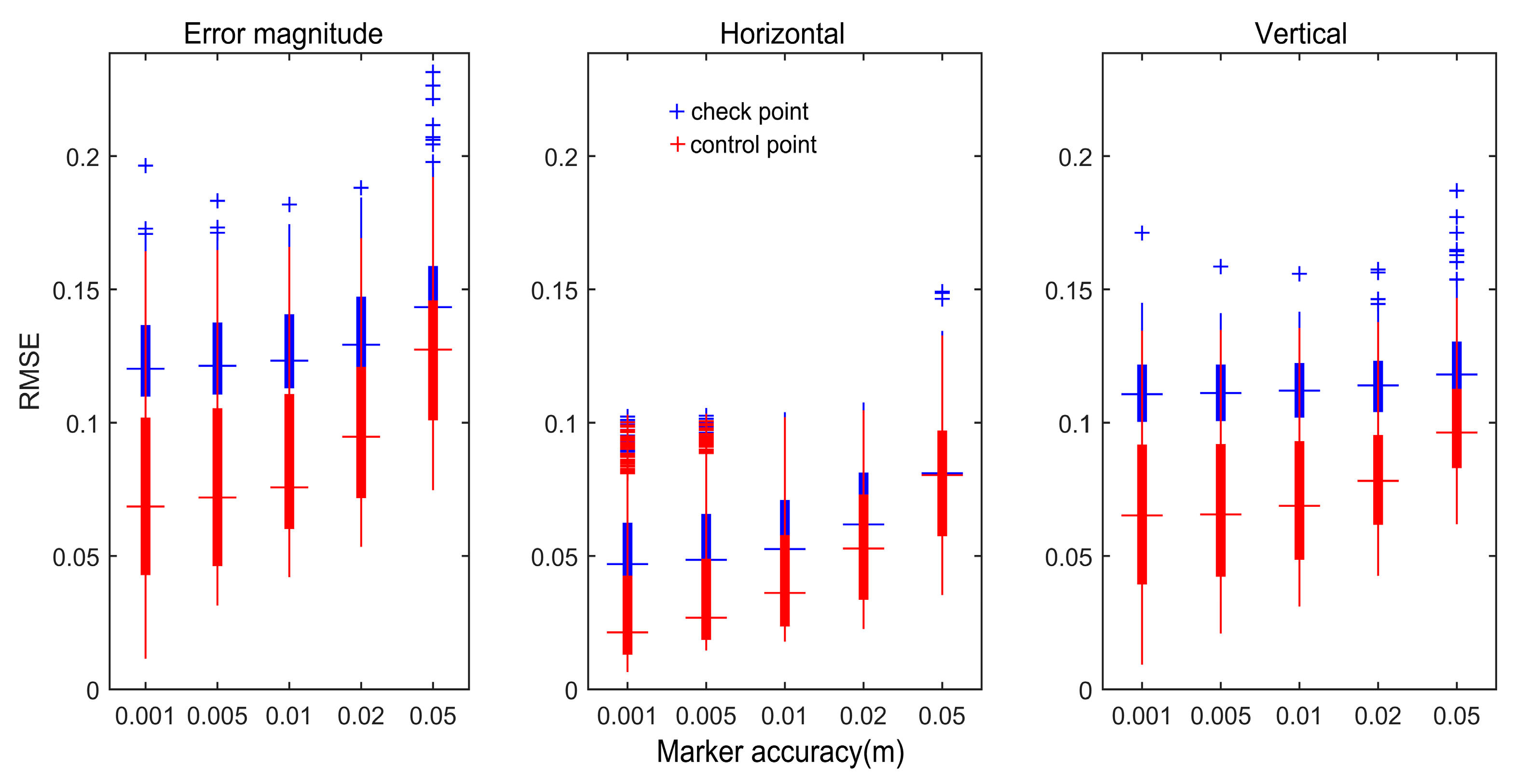
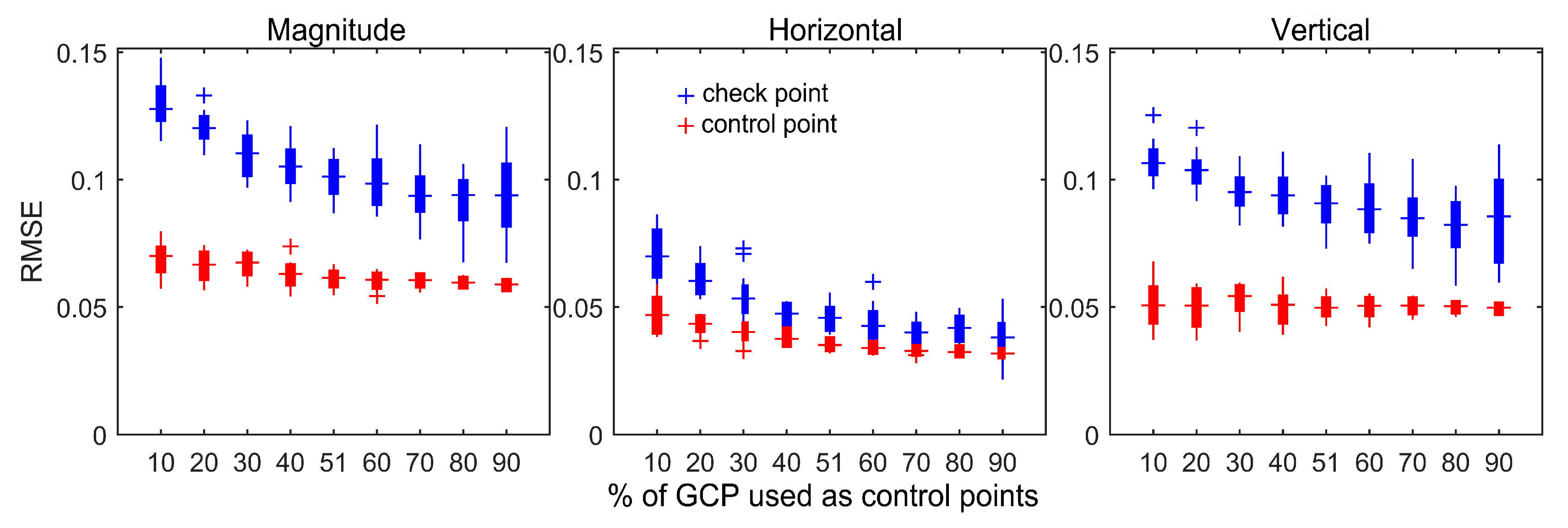
• For the generation of reference images, the different projection precision of control points and tie points applied to bundle adjustment were comprehensively compared based on the SFM method. The correlation between root means square error (RMSE) of control points and checkpoints, and the variability of spatial point precision was analyzed. Fifty percent of the ground control points (GCPs) were randomly selected as control points and 50% were used as checkpoints. The horizontal and vertical RMSEs of various GCPs and the overall RMSE were selected as control points for further analysis. Finally, the effect of the number and quality of control points on the bundle adjustment results was analyzed. These three methods were used to improve and optimize the accuracy of the DOM and DSM obtained by the UAV, and also to further improve the reliability and robustness of matching the UAV image and reference image under various complex conditions;
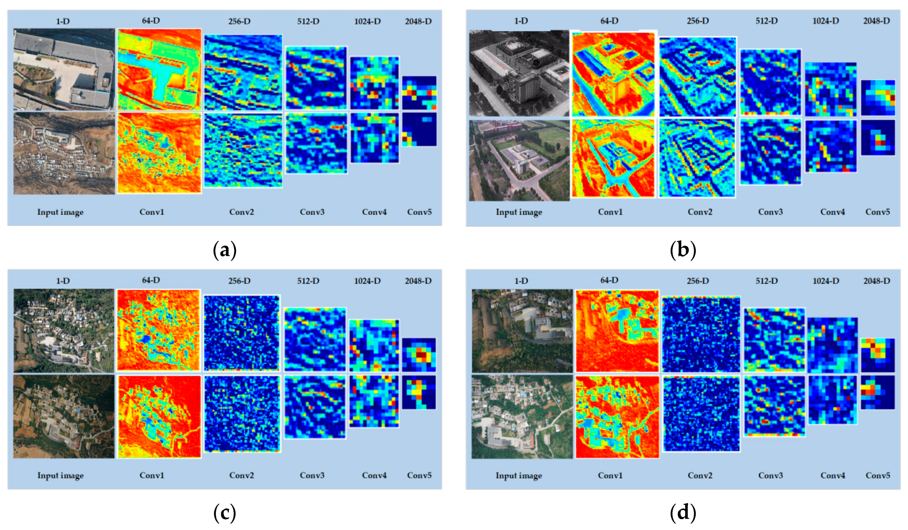
• We used transfer learning to fine-tune the pre-trained model to effectively represent deep features in air-ground multi-source images. Based on the pre-trained ResNet50 model and the high-precision experimental area reference image obtained using the SFM algorithm, a method was proposed to match UAV images and reference images by integrating multi-scale local deep features. Matching experiments were performed under various conditions, such as at various scales, viewpoints, lighting conditions, and seasons images to explore the difference in corresponding feature points between UAV images and the reference image under various complex conditions. Compared with some classic hand-crafted computer vision and deep learning methods, the proposed method provides a new solution for exploring the immediate and effective positioning of the UAV itself and ground target in GPS-denied environments.

2. Materials and Methods

2.1. Process Workflow

The accuracy of the reference image has an important impact on image geolocation. To improve the accuracy of the reference image generated from UAV sequence images, we use the stated Monte Carlo analysis and bundle adjustment algorithm to derive the reference image with higher positioning accuracy. Increasing the number of network layers is one of the methods used to improve the deep feature matching performance of CNNs. Based on previous studies, this study employed transfer learning to fine-tune the pre-trained residual neural network ResNet50 model for extracting deep features from multi-source UAV images and the reference image. The classification loss function of the output layer full CNN was used to train local deep features extracted from the UAV sequence images, and two times scale factor image pyramid was constructed to deal with scale changes. The image pyramid had a scale range from 0.125 to 2.0 with a total of 5 different levels used to obtain the regional features of images at different scales. A full CNN was applied to each level of the pyramid independently and the receptive field was configured through the convolutional layer and the pooling layer to locate the feature points. We used pixel center coordinates of the receptive field as the feature position. Local feature descriptors were obtained from feature maps which could be used to describe image local features at different scales through the use of image pyramids. Finally, we used the RANSAC algorithm to remove outliers to achieve coarse to fine image matching. The framework of our image matching workflow is illustrated in Figure 1.

2.2. Reference Image Generation

UAV images were initially processed through SFM and free network adjustment to define the network of tie points and the camera orientation. Camera self-calibration was predominantly used to adjust principal distance, image principal point, and camera radial distortion parameters [28]. The main function of the tie points between images was to identify feature point matching errors and to remove these from the free net adjustment. After the camera model was determined, photographic quality was mainly affected by the distribution density of control points, the layout method, and the accuracy of the control points. To represent the influence of control point density and distribution on the photographic quality, an appropriate number of GCPs were randomly selected as checkpoints, and then a bundle adjustment was performed [28]. Monte Carlo analysis was performed using different numbers of GCPs as control points to ascertain control point and check point error distributions. The results were used to evaluate the change in accuracy in different control density ranges. Alternatively, the error associated with any single GCP after multiple Monte Carlo iterations could be evaluated using bundle adjustment of a single control point or check point. We thus introduced the bundle adjustment (BA) model [29]. This model aimed to minimize reprojection error by adjusting the camera pose and position of spatial points [30].

For a set of control points $P_i$ in a photographic area that is continuously observed during camera movement, our goal was to calculate the pose transformation between the moving image reference frame and the fixed reference frame along with the position of all control points in the fixed reference frame. The observation equation was taken as $\mathit{z}=h\left(\mathit{x},\mathit{y}\right)$, where $\mathit{x}$ the target 3-D control point p and the observed data possess the pixel coordinates ${\left[u_s,v_2\right]}^T$ of the feature points on the image. The observation errors can then be expressed as:

$$e=z-h\left(\xi ,p\right)$$

(1)

Considering observations at other times, $z_{i,j}$ represented the data generated by observing the target point $p_j$ at pose ${\xi }_i$. The overall cost function can then be expressed as:

$$\frac{1}{2}{\displaystyle {\sum }_{i=1}^m{{\displaystyle {\sum }_{j=1}^n‖e_{ij}‖}}^2}={\displaystyle {\sum }_{i=1}^m{{\displaystyle {\sum }_{j=1}^n‖z_{ij}-h\left({\xi }_i,p_j\right)‖}}^2}$$

(2)

Minimizing this cost function requires adjustments to both the pose and the 3D target point to achieve better results.

For the overall objective function, the independent variables had to be defined as quantities to be optimized:

$$x=\left[{\xi }_1,{\xi }_2,\dots ,{\xi }_m,p_1,p_2,\dots ,p_n\right]$$

(3)

An increment of the independent variable yields the objective function:

$$\frac{1}{2}{‖f\left(x+\mathsf{\Delta }x\right)‖}^2\approx \frac{1}{2}{\displaystyle {\sum }_{i=1}^m{{\displaystyle {\sum }_{j=1}^n‖e_{ij}+F_{ij}\mathsf{\Delta }{\xi }_i+E_{ij}\mathsf{\Delta }{p}_j‖}}^2}$$

(4)

where ${\mathit{E}}_{ij}$ represents the partial derivative of the function for the target point position, and ${\mathit{F}}_{ij}$ represents the partial derivative of the function to the camera pose, linearizing the equation.

A simplified expression for the objective function can then be obtained as follows:

$$\frac{1}{2}{‖f\left(x+\mathsf{\Delta }x\right)‖}^2=\frac{1}{2}{‖e+F\mathsf{\Delta }{x}_c+E\mathsf{\Delta }{x}_p‖}^2$$

(5)

here, the Jacobian matrices $\mathit{E}$ and $\mathit{F}$ must be the derivatives of the global objective function to be global variables. They are large matrices composed of the derivatives ${\mathit{E}}_{ij}$ and ${\mathit{F}}_{ij}$ of each error term. Here, the Gauss–Newton method is used to iteratively solve the system of linear equations $\mathit{H}\mathsf{\Delta }\mathit{x}=\mathit{g}$ where:

$$H=J^{T}J=\left[\begin{array}{cc}{F}^{T}F& F^{T}E\\ E^{T}F& E^{T}E\end{array}\right]$$

(6)

The $\mathit{H}$ matrix was caused by the Jacobian matrix $\mathit{J}\left(\mathit{x}\right)$. One of cost functions ${\mathit{e}}_{ij}$ can be considered. Here it should be noted that the error term only describes an event in which the ${\mathit{T}}_i$ matrix sees ${\mathit{p}}_{\mathit{j}}$ landmark points, which involve the i-th camera pose and j-th landmark point, while the derivatives of the remaining variables are 0.

Thus, the Jacobian matrix form corresponding to this error term can thus be expressed as follows:

$$J_{ij}\left(x\right)=\left(0_{2\times 6},\dots ,0_{2\times 6},\frac{\partial e_{ij}}{\partial {\xi }_i},0_{2\times 6},\dots ,0_{2\times 3},\dots ,0_{2\times 3},\frac{\partial e_{ij}}{\partial p_i},0_{2\times 3},\dots ,0_{2\times 3}\right)$$

(7)

The specific derivation of this formula is given above, where the $0_{2\times 6}$ matrix represents a $0$ matrix with 2 × 6 dimensions. The error partial deviation $\partial {\mathit{e}}_{ij}/\partial {\xi }_i$ of the camera, the pose was 2 × 6, and the partial deviation $\partial {\mathit{e}}_{ij}/\partial {\mathit{p}}_{\mathit{j}}$ of the landmarks was 2 × 3. The Jacobian matrix of this error term was 0 except for two non-zero blocks.

Then, we used the Levenberg–Marquart iterative method for iterative optimization after obtaining $\mathsf{\Delta }x$. Here the sparseness was used to block the $\mathit{H}$ matrix to separate camera pose and landmarks, where:

$$\left[\begin{array}{cc}{H}_{11}& H_{12}\\ H_{12}^T& H_{22}\end{array}\right]\left[\begin{array}{c}\mathsf{\Delta }{x}_1\\ \mathsf{\Delta }{x}_2\end{array}\right]=\left[\begin{array}{c}{b}_1\\ b_2\end{array}\right]$$

(8)

After elimination, the first line of the equation becomes a term that has nothing to do with $\mathsf{\Delta }{x}_2$. This was taken out separately to yield the incremental equation associated with the pose as follows:

$$\left(H_{11}-H_{12}{H}_{22}^{-1}{H}_{12}^T\right)\mathsf{\Delta }{x}_1=b_1-H_{12}{H}_{22}^{-1}{b}_2$$

(9)

Finally, we took the solution of the linear equation $\mathsf{\Delta }{x}_1$ into the landmark partial incremental equation $H_{12}^T\mathsf{\Delta }{x}_1+H_{22}\mathsf{\Delta }{x}_2=b_2$, and solved for $\mathsf{\Delta }{x}_2$. Thus far, we optimized the camera pose and control points using bundle adjustment.

2.3. Image Deep Feature Extraction

In the image deep feature extraction process, the correlation between local features was measured by training a feature classifier with an attention mechanism. In [31], each feature learned a scoring function $\alpha \left(f_n;\theta \right)$, where $\theta$ was the parameter of the scoring function $\alpha \left(·\right)$. To achieve this training, weighted sum pooling was used to process features during training, where the pooling weights were obtained using the attention score network. The training process was described as continuously iterating $f_n\in R^d$, n = 1, …, N, where d represented the feature dimension, and learning together with the attention score model. The output y of the network was generated by weighted summation of feature vectors and given by:

$$y=W\left({\displaystyle {\sum }_{n}a\left(f_n;\theta \right)}·f_n\right)$$

(10)

where $W\in R^{M\times d}$ represents the final fully connected layer weight of the CNN used to train and predict the M class.

The training process used the cross-entropy loss method, which is expressed as:

$$\eta =-y^{\ast }·\log \left(\frac{\exp \left(y\right)}{1^T\exp \left(y\right)}\right)$$

(11)

where $y^{\ast }$ is the corresponding truth value, $1$ is a unit vector, and the parameters of the scoring function $\alpha \left(·\right)$ are trained using the backpropagation algorithm. Its gradient was calculated as follows:

$$\frac{\partial \eta }{\partial \theta }=\frac{\partial \eta }{\partial y}{\displaystyle {\sum }_n\frac{\partial y}{\partial a_n}\frac{\partial a_n}{\partial \theta }}=\frac{\partial \eta }{\partial y}{\displaystyle {\sum }_{n}W{f}_n\frac{\partial a_n}{\partial \theta }}$$

(12)

where the backpropagation parameter $\theta$ of the output function ${\alpha }_n=a\left(f_n;\theta \right)$ has the same meaning as the parameters of a standard multi-layer perceptron, both representing the weight $W_{\mathrm{n}+1}$ corresponding to the n + 1 node with an input of 1.

2.4. Image Matching Process

We extracted feature keypoints and descriptors from the image database, and the feature with the highest attention score in each image was selected. Based on the feature nearest-neighbor search method, the k-d tree bottom-up backtracking strategy was used to find the feature vector closest to the search target in the database. The distance between the search image feature vector and the database feature vector was the Euclidean distance between the vectors calculated from the symmetrical distance. The symmetrical distance $d\left(x;y\right)$ between the query vector x and the feature database vector y was expressed by the centroid distance between them. The equation used to calculate the symmetrical distance is as follows:

$$d\left(x;y\right)=d\left(q\left(x\right),q\left(y\right)\right)=\sqrt{{\displaystyle {\sum }_{j}d{\left(q_j\left(x\right),q_j\left(y\right)\right)}^2}}$$

(13)

where $d{\left(q_j\left(x\right),q_j\left(y\right)\right)}^2$ can be obtained by referencing the fast lookup table of the j-th sub-quantizer. Each lookup table contained the squared distance between all centroids in the sub-quantizer.

After the features to be matched were extracted from the search image, local feature descriptors that were automatically extracted from the search image were used to perform a nearest neighbor search. For the first K-nearest neighbor, local descriptors retrieved from the database, all matches for each database image were then summarized. Finally, an Affine transformation model was used to calculate the feature corresponding points in the search image and the reference image, and geometric verification based on RANSAC was performed to eliminate mismatches. The number of corresponding points in use as the final matching result was based on the image deep features.

3. Experiments and Analysis

In this section, experiments performed on several different UAV images and Google images are described to evaluate the number of correct matching points, matching precision, matching time, and robustness of our method. To evaluate the performance, camera calibration and UAV reference image data production were performed. Then, UAV images and reference image deep features were extracted and feature map visual results were presented. We also displayed the matching results for the different variations. Finally, we compared the proposed method with eight state-of-the-art image matching algorithms, including five classic hand-crafted computer vision image matching methods (SIFT [4], SURF [5], ORB [6], AKAZE [7], RIFT [32]), and three deep-learning image matching methods (LPM [33], R2D2 [34], SuperPoint [35]).

3.1. Data Source

The experimental data were obtained from the UAV platform and Google Earth, and the overall terrain in the experimental area was low hills with moderate elevation differences and rich ground object types, which were conducive to verification robustness of the UAV image and reference image matching algorithm. However, the UAV platform is limited by the sensor field of view, and when acquiring a wide range of terrain data, it needs to fly multiple routes to acquire all images in the survey to ensure the overlap of the image data. The data source of the experimental UAV reference image was obtained from UAV sequence images with 80% photographic course overlap and 60% lateral overlap. The sequence images include top views at 1:500 and 1:1000 scales, oblique views at different illumination and different seasons, and oblique views at different scales and different viewpoints. The Google reference image was obtained from the Google Earth platform.

3.2. Experiment Platform

The experiments were performed on a 2.6GHz Intel CPU with 32GB RAM, NVIDIA GTX 1660Ti, Win10 PC. The programming environment used was Anaconda3 5.2.0 (https://mirrors.tuna.tsinghua.edu.cn/anaconda/archive/) (accessed on 20 December 2021) with TensorFlow 1.2.0.

3.3. UAV Reference Image

Camera calibration is a key link in camera measurement applications. The accuracy of the calibration results affects the convenience and accuracy of the image [36]. In our experiment, the average and standard deviation of parameters in the camera were obtained based on the results of multiple self-calibrations using the Agisoft Metashape software. The purpose was to make an image network for self-calibration to perform the strict quality estimation. The results are shown in

Table 1. Camera calibration results.

Camera Parameter	Calibrate Values
Model	DSC-RX1RM2
Image size	7952 × 5304 pixels
Focal length	35 mm
Pixel size	4.53 μm
Principal distance	7507.03 ± 11.41 pixels
$f_x$ and $f_y$	7752.36 ± 17.65 mm
$\left(c_x, c_y\right)$	(7.05 ± 0.94, −43.71 ± 2.04) mm
$k_1$	−0.04 ± 0.05
$k_2$	−0.22 ± 0.57
$k_3$	0.33 ± 0.22

.

In the case of fixed camera calibration, the parameter size settings of the tie point accuracy, GCP projection accuracy, and marker accuracy during the UAV image processing have an important impact on the self-calibrated bundle adjustment results. To describe this effect and determine a better marker accuracy value, we selected 12 GCPs as checkpoints and 82 GCPs as control points. We then performed unified bundle adjustment and calculated the range of adjustment results. The setting range for tie point accuracy and projection accuracy was 0.1–4.0 and 0.1–1.0 pixels, respectively. Marker accuracy was set to 0.001, 0.005, 0.01, 0.02, and 0.05. As shown in Figure 2, the results showed that the RMSE value of the control points was between 0–0.25 m and the RMSE value of the checkpoints was concentrated in the range 0.10–0.15 m. It reflected the strong spatial variation of RMSE, and the uneven distribution of the observation weights of the GCPs. The RMSE ratio (check/control and control/check) between check points and control points was helpful in terms of confirming whether the error distribution was consistent during the bundle adjustment process because a larger RMSE value indicated an overfit to the control point measurement. In Figure 2, we show the ratio surface graph of an average checkpoint and control point RMSE value for each marker accuracy in detail.

Figure 3 shows the RMSE results of the bundle adjustment combined with the control points and checkpoints from the stated Monte Carlo analysis, where each box wireframe represents the results of the five self-calibration bundle adjustments performed with a specific marker accuracy. The horizontal line indicates the median RMSE. The boxes were distributed at 25% and 75% positions and the whiskers represent the full range of adjustment results. They are not regarded as outliers and are represented by the “+” sign.

The experimental results showed that as the marker accuracy value continued to increase, the box of the control point RMSE kept growing and its median value also increased. In particular, when the marker accuracy value was greater than 0.01, the RMSE value changed significantly. The marker accuracy value always kept the RMSE values in the horizontal direction low. There was not much of a difference between the control point and checkpoint values. The RMSE value in the vertical direction was significantly higher than in the horizontal direction. As the difference between the control point and check point increased, the “+” sign of whiskers value increased. In general, the RMSE values of the control points and check points remained relatively stable and the median showed no significant change. The marker accuracy value was 0.01 m as the boundary. When its accuracy was greater than 0.01 m, the RMSE values of the control points and check points were significantly increased, its accuracy was greater than 0.01 m, and the RMSE values of the control points and check points were significantly increased. When its accuracy was less than 0.01 m, the RMSE value remained stable. To reduce the marker accuracy constraint value and improve the RMSE accuracy of the bundle adjustment and remove the abnormal values, the marker accuracy value was set to 0.01 m in the experiment.

Based on the results of the stated Monte Carlo analysis, we obtained values for the projection accuracy, tie point accuracy, and marker accuracy that could be used to balance the bundle adjustment results. To further improve the bundle adjustment accuracy, a specific number of different, randomly selected GCPs were used as control points for each bundle adjustment and the remaining GCPs were used as checkpoints. The result was determined by performing 20 adjustment iterations per analysis procedure. In our experiment, a random selection of 10–90% of the GCPs was used as control points for each bundle adjustment analysis procedure. The results of the stated Monte Carlo box analysis are shown in Figure 4. As can be seen, the density of any specific control points and the distribution of the RMSE values reflected the changes caused by the specific selection of GCPs for control points or checkpoints. For regional network bundle adjustments involving any number of control points, the change in RMSE value reflected the change in results associated with selecting different control points. This figure also shows the inverse correlation between the RMSE value and the proportion of control points. This indicated that the overall error could be minimized by not allowing more control points to participate in the regional network bundle adjustment. A small number of control points participating in bundle adjustment will reduce the regional network constraints during the adjustment to make the control point RMSE value smaller, which will also cause the control point and checkpoint RMSE box to become more separated. Because fewer GCPs were used as control points, the margin of error between the control points and checkpoints varied. This constraint can be better adapted to bundle adjustment by reducing the number of control points, resulting in a small control point RMSE value. However, the use of only a few GCPs as control points increases the difficulty associated with providing effective constraints for the bundle adjustment of large areas, causing checkpoints to vary widely. Reducing the number of control points participating in adjustment gradually increases the checkpoint error. Additionally, horizontal and vertical errors are highly systematic, reflecting the fact that the positioning accuracy of UAV images depends on control point distribution. Therefore, we believe that adjustment using more than 80% of the GCPs as control points can effectively minimize the impact of any spatially weaker control point distribution based on the analysis results for each GCP.

Accuracy maps provide valuable insights into predicted photographic areas and highlight the impact of photogrammetry and georeferencing on overall photographic quality [37]. Therefore, the evaluation of the correlation between parameters can provide insight into any self-calibration problems. Experimentally, the control point position is measured using the global navigation satellite system (GNSS) to provide absolute position and accuracy (accuracy is better than 2 mm in the horizontal direction and better than 1cm in the vertical direction). Based on the Agisoft Metashape software used for UAV image data processing, other parameter values were set as follows: the accuracy of photo alignment was “medium”, and the limit to the number of tie points was set to 4000 to provide a tight distribution of tie points for accurate analysis. For accuracy, dense cloud generation was performed with “high quality”, and surface noise was minimized by “aggressive” depth filtering. The final experimental results are shown in

Table 2. Characteristics of the experimental area surveys.

Survey Parameters		Values
Flight plan	Altitude	350 m
	Image overlap	80% forward 60% side
Camera orientations	Position (X, Y, Z; m)	[0.029, 0.032, 0.025]
	Rotation (roll, pitch, yaw; mdeg.)	[0.005, 0.004, 0.002]
Processing	Number of images processed	327
	GCPs (as control, [as check])	82 [12]
	GCP image precision (pix)	0.1
	Tie point image precision (pix)	0.75
GCP RMS discrepancies	Control points (X, Y, Z; m)	[1.772, 1.603, 0.054]
	Check points (X, Y, Z; m)	[0.758, 0.186, 0.388]
Point coordinate RMS discrepancies	Mean for all points (X, Y, Z; mm)	0.72
	Std. deviation all points (X, Y, Z; mm)	0.57

.

Based on the above analysis, the final projection accuracy was set to 0.1 pixel, tie point accuracy was 0.75 pixel, marker accuracy was 0.01 m, 80% of the GCPs were selected as control points, and 20% of the GCPs were used as check points. The DOM and DSM of the study area are shown in Figure 5.

3.4. Deep Feature Visualization

This study aimed to improve the accuracy and robustness of collaborative matching between multi-source image deep features. An optical HD camera and infrared thermal imager were used for collecting experimental data. The purpose was to verify the performance of our algorithm for the collaborative matching of visible images and thermal infrared images with a reference image. For the bottom-up hierarchical CNN structure, different layers of neurons have learned different image feature types. The bottom layer of the hierarchy learns basic features, and the features that are extracted upward are closer to the current work. Based on the ResNet50 pre-trained model, the first 5 layers of features from the UAV sequence images and reference images were extracted after convolution. For the hierarchical CNN structure, different levels of neurons learned different types of image features, and the bottom-up features formed a hierarchical structure. The bottom layer of the hierarchy learned basic features, and the features that were extracted upward were more closely associated with the current task [16,38,39]. The image had 64-dimensional features after the first convolutional layer, 256-dimensional features after the second convolutional layer, 512-dimensional features after the third convolutional layer, 1024-dimensional features after the fourth convolutional layer, and 2048-dimensional features were obtained after the fifth convolutional layer. Figure 6 shows the feature maps of the first to the fifth layer after convolution for various matching cases.

Based on a comprehensive consideration and comparison of feature descriptor dimensions and feature complexity, we finally selected features of the fourth convolutional layer output. The input of this layer was a 28 × 28 × 512 feature map. The output feature map was upgraded by first reducing the input feature map to 28 × 28 × 256 through a 1 × 1 × 256 convolutional layer, then through a 3 × 3 × 256 convolutional layer, and finally through a 1 × 1 × 1024 convolutional layer.

3.5. Matching Results and Analysis

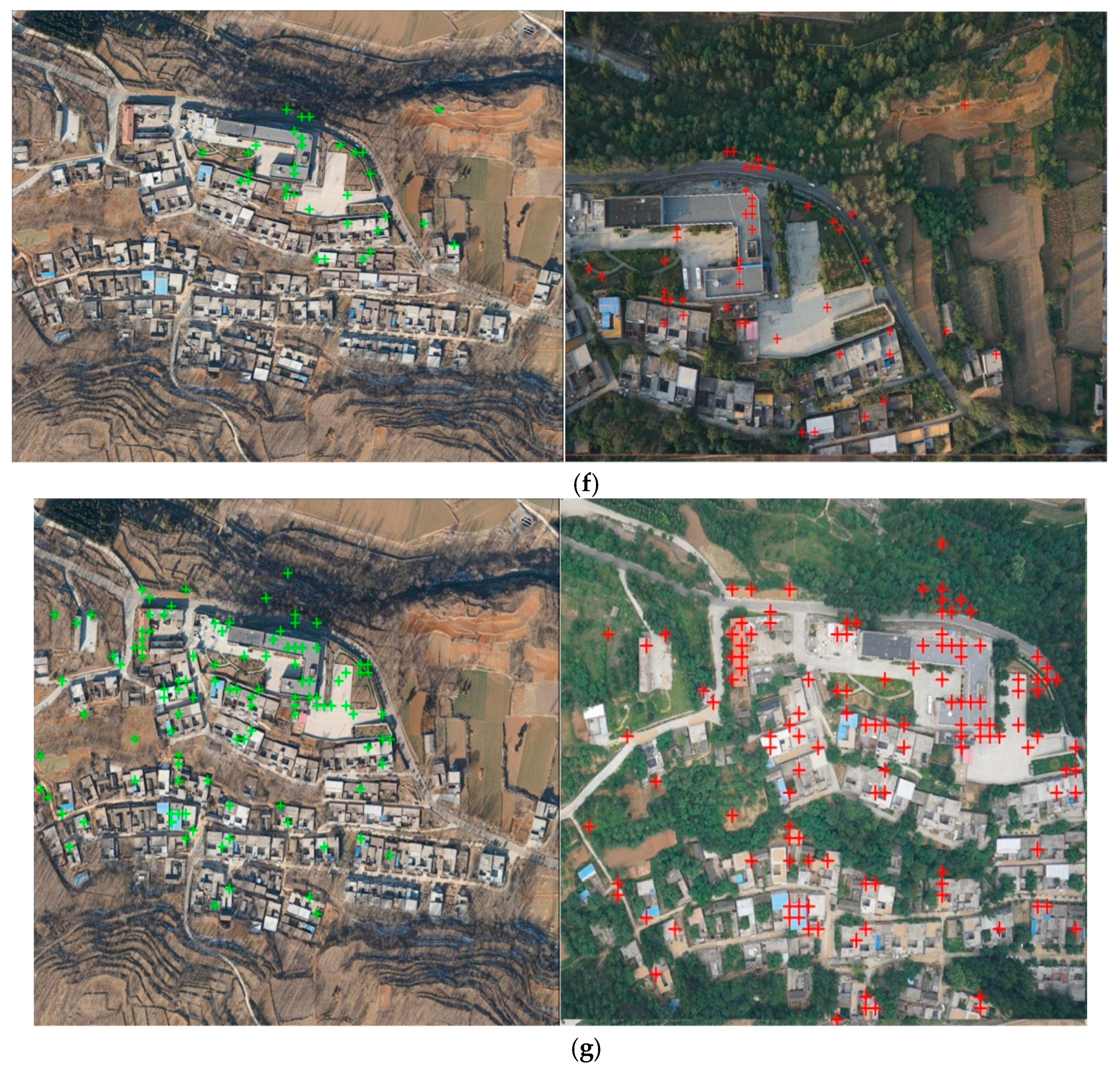
3.5.1. Matching Results Based on UAV Reference Image

In this section, experimental area DOM made using UAV images taken in winter was used as the reference image and its deep features were extracted. Experimental data were typical multi-source, multi-temporal, and multi-resolution images. We extracted local deep features from different types of UAV images and matched these with the reference image. Deep feature automatic recognition and matching system for complex conditions should be able to adapt to some environmental change and still detect natural features stably. This stability is termed repeatable detection capability, which indicates that significant feature detection capabilities are independent of environmental changes such as camera parameters, viewpoint changes, and changes in illumination. To verify the ability of the proposed method to repeatedly detect significant feature locations, deep feature matching experiments involving different scales, rotations, viewpoints, and changes in lighting conditions were performed.

Photographic images vary in scale due to changes in the camera altitude or focal length during the UAV image acquisition process. Viewpoint changes are typically divided into two types. One involves long-distance images, large tilt, and small scale to match the reference image. The other involves short distance images, small tilt, and large scale to match the reference image. Image matching feature points with large changes in viewpoint are concentrated in the central area of the image, with fewer matching points on the edges. There are two reasons for the small number of feature matching points at the edges. One is that the large tilt leads to longer distances. These greater distances lead to larger deformations, including features being hidden in some cases, making matching difficult. The second reason is that some features of an oblique image are not visible on the reference image. Illumination changes will have a great impact on the overall grayscale distribution of the image, the edge information, and the chromaticity space of the color image, which will affect the accuracy of the feature points-based scene matching methods.

In this experiment, the reference images with 10-cm resolution, along with UAV images taken at different resolutions, seasons, viewpoints, illuminations, and with different sensors were used as the images to be matched. Among these, we used some historical DOM at different periods as the target images to be matched. First, we performed scale, seasonal, viewpoint, and illumination change experiments to verify the performance of the deep feature matching, as shown in Figure 7.

Figure 7 shows the seven group images matched results based on UAV reference image in different conditions which included variations in scale, season, viewpoint, and illumination. The proposed method obtained a rich number of correct matching points, and the identified corresponding points are sufficient and evenly distributed, indicating that the proposed method has good robustness in matching multi-source images with different viewpoints, different illumination, and different scales.

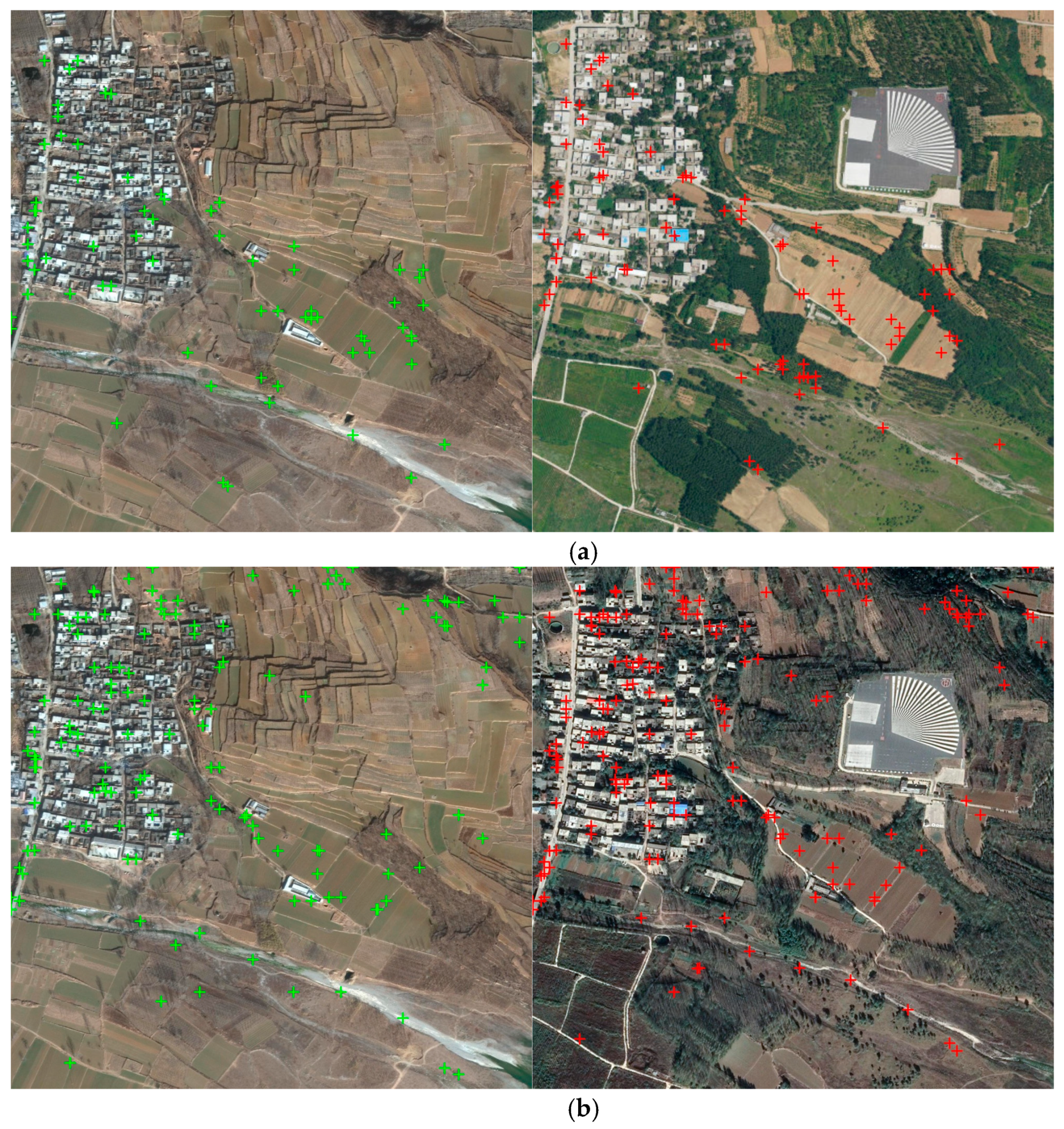
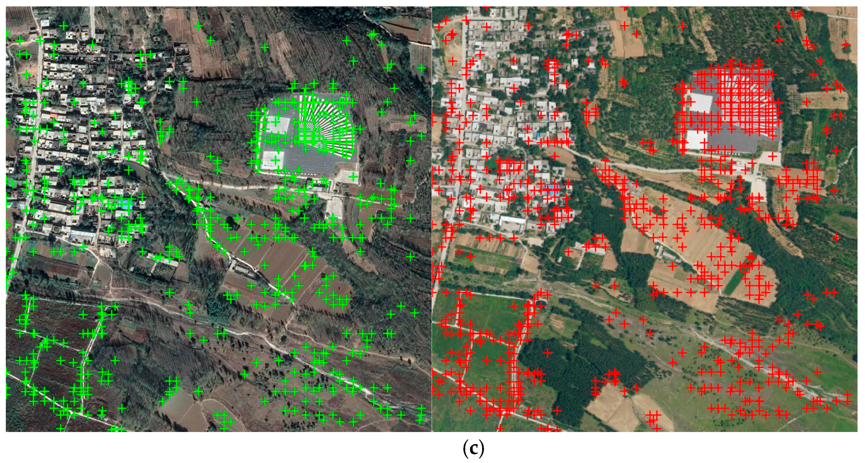
3.5.2. Matching Results Based on Google Reference Image

In this section, the reference image of the experimental area was obtained from the Google Earth platform. The experimental data had obvious multi-source and multi-temporal characteristics. We extracted local deep features from different types of images and matched these with the reference image. Image temporal changes can typically change the physical locations of matching feature points. It could cause textural differences, lighting differences, weather changes, object occlusion, and can increase or decrease the ground objects on the image. This has an important impact on the extraction of deep features. Therefore, the robustness of the image matching algorithm can be demonstrated by using images with large temporal variations to test.

Figure 8 presents the three group images matched results based on Google reference images in different conditions which included variations in season, texture, time, and season. The experimental results vividly describe the effects of image time, season, and texture changes on the performance of multi-source image matching, indicating that these features play an important role in multi-source image matching. However, the proposed method could obtain a large number of matched point pairs, and the corresponding points are evenly distributed, indicating that our algorithm has good robustness in multi-source image matching based on Google reference images with different seasons, different textures, and different times.

3.6. Matching Performance Analysis

The above experimental results showed that our method could obtain many features’ corresponding points, which all had a good distribution on the matched images. The matching was relatively dense on the search image. It displayed that the use of local deep features and transfer learning to fine-tune the ResNet50 convolutional neural network model imparted higher robustness in terms of changes in scale, season, viewpoint, and illumination. To evaluate the performance of our method more comprehensively, image matching precision and runtime are used as criteria in the evaluation. EC represented the number of coarse matching points, CC represented the number of fine matching points, and the precision criteria were defined as precision = CC/EC. The results are shown in

Table 3. Multi-source image matching results for ten cases.

Image Pair		Indicators
		EC	CC	Precision	Time(s)
Figure 7	case1	1060	215	20.3%	5.925
	case2	1040	199	19.1%	8.128
	case3	241	79	32.7%	8.281
	case4	471	141	29.9%	5.956
	case5	484	75	15.5%	7.163
	case6	383	50	13.1%	8.934
	case7	1178	138	11.7%	5.863
Figure 8	case8	1655	87	5.3%	7.371
	case9	2157	140	6.5%	6.301
	case10	2448	949	38.7%	7.359

. We found that the image matching had higher precision and a lower time cost, indicating that the proposed method can adapt more effectively to multi-source remote sensing image matching. In matching results based on UAV reference, the highest precision is viewpoint change in case 3, up to 32.7%, the lowest precision is rainy illumination in case 7, only 11.7%. In addition, the matching precisions of case 5 and case 6 with overcast and sunset illumination are also relatively low. In matching results based on Google reference image, case 10 with more significant similarity had the best matching result, showing that the higher the image similarity, the better the matching effect. It demonstrated that the light and the seasonal difference had a great impact on the coarse and fine matching pairs of multi-source images.

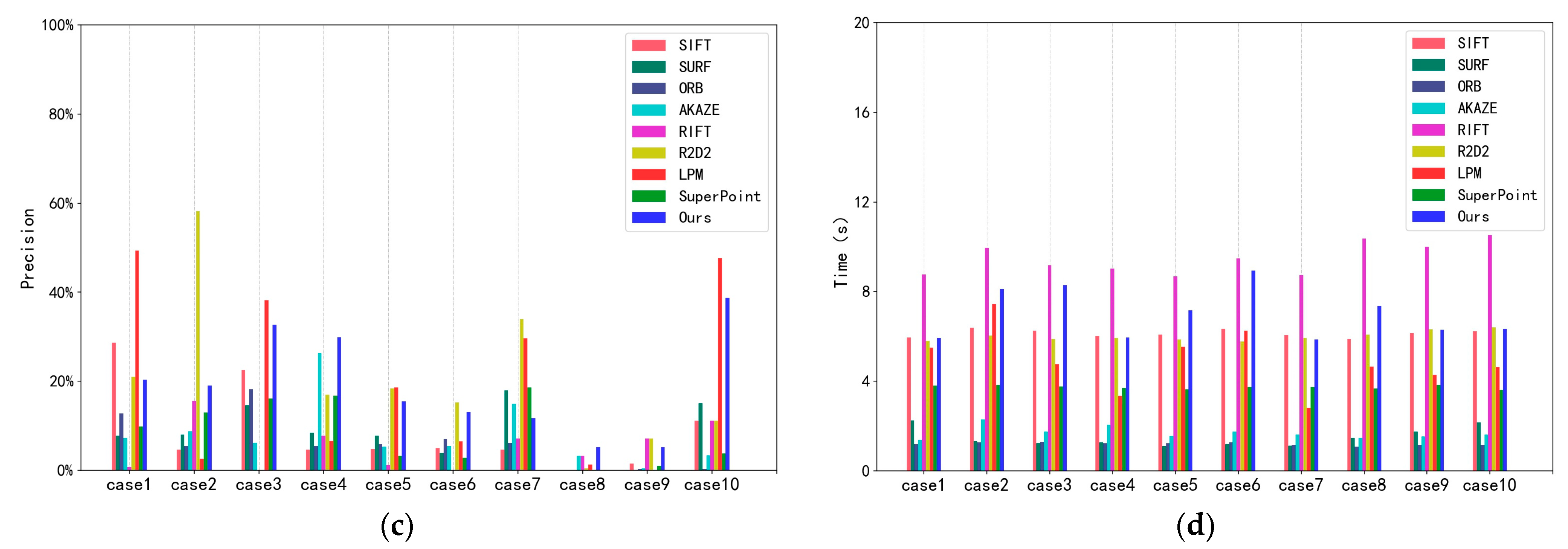
3.7. Matching Performance Comparison

To demonstrate the advantages of the proposed method, comparative experiments with some popular image matching methods were conducted, including five hand-crafted matching methods (SIFT, SURF, ORB, AKAZE, RIFT) and three deep learning matching methods (LPM, R2D2, SuperPoint). SIFT and SURF descriptors were searched using the fast approximately nearest neighbor method and the Euclidean distance was used for similarity measurements. The AKAZE descriptor was searched using a brute force search and similarity measurements were performed using the Euclidean distance. The ORB feature was searched using a brute force search, and the Hamming distance was used for similarity measurements. For these algorithms, we directly used the relevant functions provided by OpenCV version 3.4.2.16, and the feature detection value was set to 5000. The description and matching were left as default values. The parameters setting of RIFT, R2D2, LPM, and SuperPoint methods follow the original paper for a fair comparison. We performed a comparison with the above-mentioned hand-crafted and deep learning methods in terms of the number of coarse and fine matches, matching precision, and matching time. Experimental results are shown in Figure 9. From the experimental results, we found that the hand-crafted matching algorithms provided by OpenCV library are difficult to adapt to multi-source image matching, because the fine matching numbers and the matching precision are low. The performance of deep learning methods varies significantly in different cases. The proposed method could obtain a lot of fine matching corresponding points in all cases. It is a significant advantage of the proposed method. The fine matching number was always at a high level, and the stability was better than other algorithms. Therefore, the proposed method achieved good matching precision, which shows that it is suitable for multi-source image matching. In terms of matching time consumption, the runtime of our method was relatively low and it was slightly higher than other matching methods (SURF, ORB, AKAZE, SuperPoint) which are known for matching speed, but the fine matching numbers and matching precision were much higher than these methods. Comprehensive analysis shows that the proposed method has better robustness for multi-source image matching.

4. Discussion

This study involved the use of local deep features based on transfer learning to fine-tune a pre-trained ResNet50 convolutional neural network model matching framework. This was used to effectively find matches between the reference image and multi-source UAV images with complex background variations to solve the problem of UAV self- and target-positioning in GPS-denied environments. The experimental results showed that our method was effective. The following steps were included in the proposed method.

Firstly, we obtained search images from different sensors at different periods, such as oblique views at different seasons and illuminations, and oblique views at different scales and viewpoints. Then, we combined the best practice of the SFM algorithm and Monte Carlo analysis through free net adjustment and bundle adjustment. We found the optimal control point projection accuracy, tie point accuracy, and mark accuracy to improve the DSM and DOM accuracy of the study area.

Secondly, we fine-tuned the output feature vector of the pre-trained ResNet50 model to extract the deep features from multi-source UAV images and reference images. Then, a five-layer image pyramid model with two times scaling factor was used to solve the problem of image multi-scale deep feature extraction. The method was also used to perform multi-scale, multi-seasonal, multi-viewpoint matching of air-ground images.

Finally, a coarse-to-fine image matching strategy based on the RANSAC constraint algorithm for multi-source UAV images and reference images was applied.

The precision of the UAV reference image depends on the projection accuracy, tie point accuracy, marker accuracy, image texture, camera model, and camera geometry. In our experimental results, the large changes in control point RMSE and checkpoint RMSE were caused by changing the input control and tie point image observation accuracy setting for processing (Figure 2), which illustrated the importance of the settings. Therefore, appropriate observation accuracy values need to be used to avoid introducing processing errors into the DSM and DOM. Suitable values for tie and control points can be determined from the RMSE image residual magnitudes computed from the bundle adjustment. Through using appropriate values for the tie point and GCP image projection accuracy, the difference in DSM and DOM RMSE with different GCPs improved from 15.9 to 3 mm, which could be considered an improvement by a factor of 5.3 in precision. Appropriate setting values resulted in the check point RMSE decreasing from 17 to 8.8 mm, representing an improvement in accuracy of approximately 2 times. The Monte Carlo analysis suggested that the assessed performance would not be substantially degraded if 50% fewer GCPs had been deployed (Figure 4). This would also provide significant GCP redundancy in terms of using the Monte Carlo approach for validating the quality. Our approach highlights the utility of processing different GCPs and check point combinations to demonstrate a reduction in the error associated with the bundle adjustment and provides a more reliable reference image generation solution.

To acquire sufficient matches with good distribution, we used the transfer learning method to fine-tune the pre-trained ResNet50 model with Google’s landmark dataset and extracted the first 5 block layers of deep features from the convolutional layer module. We selected descriptors of the fourth block convolutional layer output result, which the 1024-dimension feature descriptors for initial image matching were used along with RANSAC to achieve coarse-to-fine matching. The image matching pairs covered diverse scenarios which included multi-scale, multi-season, and multi-viewpoint scene changes of the study area. The results indicated that the proposed method was more effective and stable in terms of multi-source remote sensing image matching than some state-of-the-art hand-crafted computer vision methods and deep learning matching methods.

However, the reference image was generated from UAV sequence images, which are still difficult to adapt in unfamiliar areas. Therefore, we supplemented it with Google image as the reference image and got good results. Experimental results showed that the proposed method could still obtain a good matching effect based on the Google reference image. To realize engineering application, based on the findings and explorations in this study, developing a real-time UAV pose estimation method using the deep feature of the satellite image is the next step of our research.

5. Conclusions

In this paper, a learning feature matching method was proposed based on the pre-trained ResNet50 model. The matching experiments were conducted under various conditions such as different scales, different views, different illumination, and different seasons. The results showed that the proposed method can obtain efficient and robust results in UAV image and reference image matching under various complex conditions, and has obvious advantages over some classical hand-crafted and deep learning methods. It is valuable to solve UAV self- and target-geolocation based on image feature matching in GPS-denied environments.

However, the pre-trained ResNet50 model is limited by the time cost, which makes it difficult to achieve real-time matching. Deep learning features are data-driven feature representations, and a large amount of training data is often required to obtain convolutional neural network models with powerful feature representation. In addition, the accuracy of deep learning feature recognition and detection significantly depends on the quality and variety of training datasets. Therefore, we can further exploit the idea of transfer learning to find a pre-trained lightweight network and some labeled data which is close to the target dataset, while using these models and data to build a model that would increase the labeling of target data to achieve real-time image matching. Our future work will focus on improving the efficiency of the matching algorithm of the proposed method to reduce time costs.

References

1. Kim, D.; Nam, W.; Lee, S. A Robust Matching Network for Gradually Estimating Geometric Transformation on Remote Sensing Imagery. In Proceedings of the 2019 IEEE International Conference on Systems, Man and Cybernetics (SMC), Bari, Italy, 6–9 October 2019; pp. 3889–3894. [Google Scholar]
2. Gruen, A. Development and Status of Image Matching in Photogrammetry. Photogramm. Rec. 2012, 27, 36–57. [Google Scholar] [CrossRef]
3. Liu, Y.; Mo, F.; Tao, P. Matching Multi-Source Optical Satellite Imagery Exploiting a Multi-Stage Approach. Remote Sens. 2017, 9, 1249. [Google Scholar] [CrossRef] [Green Version]
4. Lowe, D.G. Distinctive image features from scale-invariant keypoints. Int. J. Comput. Vis. 2004, 60, 91–110. [Google Scholar] [CrossRef]
5. Bay, H.; Tuytelaars, T.; van Gool, L. Surf: Speeded up robust features. In Proceedings of the European Conference on Computer Vision, Graz, Austria, 7–13 May 2006; pp. 404–417. [Google Scholar]
6. Rublee, E.; Rabaud, V.; Konolige, K.; Bradski, G.R. ORB: An efficient alternative to SIFT or SURF. In Proceedings of the International Conference on Computer Vision, Barcelona, Spain, 6–13 November 2011; pp. 2564–2571. [Google Scholar]
7. Alcantarilla, P.F.; Bartoli, A.; Davison, A.J. KAZE features. In Proceedings of the European Conference on Computer Vision, Florence, Italy, 7–13 October 2012; pp. 214–227. [Google Scholar]
8. Wu, Y.; Di, L.; Ming, Y.; Lv, H.; Tan, H. High-Resolution Optical Remote Sensing Image Registration via Reweighted Random Walk Based Hyper-Graph Matching. Remote Sens. 2019, 11, 2841. [Google Scholar] [CrossRef] [Green Version]
9. Bruce, L.M.; Koger, C.H.; Li, J. Dimensionality reduction of hyperspectral data using discrete wavelet transform feature extraction. IEEE Trans. Geosci. Remote Sens. 2002, 40, 2331–2338. [Google Scholar] [CrossRef]
10. Zabalza, J.; Ren, J.; Yang, M.; Zhang, Y.; Wang, J.; Marshall, S.; Han, J. Novel folded-PCA for improved feature extraction and data reduction with hyperspectral imaging and SAR in remote sensing. ISPRS J. Photogramm. Remote Sens. 2014, 93, 112–122. [Google Scholar] [CrossRef] [Green Version]
11. Cheng, G.; Han, J. A Survey on Object Detection in Optical Remote Sensing Images. ISPRS J. Photogramm. Remote Sens. 2016, 177, 11–28. [Google Scholar] [CrossRef] [Green Version]
12. Jégou, H.; Douze, M.; Schmid, C. Improving Bag-of-Features for Large Scale Image Search. Int. J. Comput. Vis. 2010, 87, 316–336. [Google Scholar] [CrossRef] [Green Version]
13. Fan, D.; Dong, Y.; Zhang, Y. Satellite Image Matching Method Based on Deep Convolutional Neural Network. J. Geod. Geoinf. Sci. 2019, 2, 90–100. [Google Scholar]
14. Xiao, X.; Guo, B.; Li, D.; Li, L.; Yang, N.; Liu, J.; Zhang, P.; Peng, Z. Multi-View Stereo Matching Based on Self-Adaptive Patch and Image Grouping for Multiple Unmanned Aerial Vehicle Imagery. Remote Sens. 2016, 8, 89. [Google Scholar] [CrossRef] [Green Version]
15. Yuan, W.; Yuan, X.; Xu, S.; Gong, J.; Shibasaki, R. Dense Image-Matching via Optical Flow Field Estimation and Fast-Guided Filter Refinement. Remote Sens. 2019, 11, 2410. [Google Scholar] [CrossRef] [Green Version]
16. Li, K.; Zhang, Y.; Zhang, Z.; Lai, G. A Coarse-to-Fine Registration Strategy for Multi-Sensor Images with Large Resolution Differences. Remote Sens. 2019, 11, 470. [Google Scholar] [CrossRef] [Green Version]
17. Ling, X.; Huang, X.; Zhang, Y.; Zhou, G. Matching Confidence Constrained Bundle Adjustment for Multi-View High-Resolution Satellite Images. Remote Sens. 2020, 12, 20. [Google Scholar] [CrossRef] [Green Version]
18. Swaroop, A.; Aman, A.R.; Giri, A.; Gothwal, H. Content-Based Image Retrieval: A Comprehensive Study. Int. J. Sci. Res. Comput. Sci. Eng. Inf. Technol. 2019, 5, 1073–1081. [Google Scholar]
19. Oquab, M.; Bottou, L.; Laptev, I.; Sivic, J. Learning and transferring mid-level image representations using convolutional neural networks. In Proceedings of the IEEE Conference on Computer Vision and Pattern Recognition, Columbus, OH, USA, 23–28 June 2014; pp. 1717–1724. [Google Scholar]
20. Guo, Y.; Shi, H.; Kumar, A.; Grauman, K.; Rosing, T.; Feris, R. SpotTune: Transfer learning through adaptive fine-tuning. In Proceedings of the IEEE Conference on Computer Vision and Pattern Recognition, Long Beach, CA, USA, 15–20 June 2019; pp. 4805–4814. [Google Scholar]
21. Al-Ruzaiqi, S.K.; Dawson, C.W. Optimizing Deep Learning Model for Neural Network Topology. In Intelligent Computing—Proceedings of the Computing Conference, London, UK, 16–17 July 2019; Arai, K., Bhatia, R., Kapoor, S., Eds.; Springer: Cham, Switzerland, 2019; pp. 785–795. [Google Scholar]
22. Tajbakhsh, N.; Shin, J.Y.; Gurudu, S.R.; Hurst, R.T.; Kendall, C.B.; Gotway, M.B.; Liang, J. Convolutional neural networks for medical image analysis: Full training or fine tuning? IEEE Trans. Med. Imaging 2016, 35, 1299–1312. [Google Scholar] [CrossRef] [Green Version]
23. Maggiori, E.; Tarabalka, Y.; Charpiat, G.; Alliez, P. Convolutional neural networks for large-scale remote-sensing image classification. IEEE Trans. Geosci. Remote Sens. 2016, 55, 645–657. [Google Scholar] [CrossRef] [Green Version]
24. Yosinski, J.; Clune, J.; Bengio, Y.; Lipson, H. How transferable are features in deep neural networks? Adv. Neural Inf. Process. Syst. (NIPS) 2014, 27, 3320–3328. [Google Scholar]
25. Lucey, S.; Goforth, H. GPS-Denied UAV Localization using Pre-existing Satellite Imagery. In Proceedings of the International Conference on Robotics and Automation (ICRA), Montreal, QC, Canada, 20–24 May 2019. [Google Scholar]
26. Nassar, A.; Amer, K.; ElHakim, R.; ElHelw, M. A Deep CNN-Based Framework For Enhanced Aerial Imagery Registration with Applications to UAV Geolocalization. In Proceedings of the Computer Vision & Pattern Recognition Workshops, Salt Lake City, UT, USA, 18–22 June 2018. [Google Scholar]
27. Ma, J.; Jiang, X.; Fan, A.; Jiang, J.; Yan, J. Image Matching from Handcrafted to Deep Features: A Survey. Int. J. Comput. Vis. 2021, 129, 23–79. [Google Scholar] [CrossRef]
28. James, M.R.; Robson, S.; d’Oleire-Oltmanns, S.; Niethammer, U. Optimising UAV topographic surveys processed with structure-from-motion: Ground control quality, quantity and bundle adjustment. Geomorphology 2017, 280, 51–66. [Google Scholar] [CrossRef] [Green Version]
29. Alismail, H.; Browning, B.; Lucey, S. Photometric bundle adjustment for vision-based slam. In Proceedings of the Asian Conference on Computer Vision, Taipei, Taiwan, 20–24 November 2016; pp. 324–341. [Google Scholar]
30. Hartley, R.; Zisserman, A. Multiple View Geometry in Computer Vision; Cambridge University Press: Cambridge, UK, 2003. [Google Scholar]
31. Noh, H.; Araujo, A.; Sim, J.; Weyand, T.; Han, B. Large-Scale Image Retrieval with Attentive Deep Local Features. In Proceedings of the 2017 International Conference on Computer Vision, Venice, Italy, 22–29 October 2017. [Google Scholar]
32. Li, J.; Hu, Q.; Ai, M. RIFT: Multi-Modal Image Matching Based on Radiation-Variation Insensitive Feature Transform. IEEE Trans. Image Process. 2020, 29, 3296–3310. [Google Scholar] [CrossRef]
33. Ma, J.; Jiang, J.; Zhou, H.; Zhao, J.; Guo, X. Guided locality preserving feature matching for remote sensing image registration. IEEE Trans. Geosci. Remote Sens. 2018, 56, 4435–4447. [Google Scholar] [CrossRef]
34. Revaud, J.; Weinzaepfel, P.; Souza, C.D.; Pion, N. R2D2: Repeatable and Reliable Detector and Descriptor. In Proceedings of the Thirty-third Conference on Neural Information Processing Systems, Vancouver, BC, Canada, 8–14 December 2019. [Google Scholar]
35. DeTone, D.; Malisiewicz, T.; Rabinovich, A. SuperPoint: Self-Supervised Interest Point Detection and Description. In Proceedings of the IEEE Conference on Computer Vision and Pattern Recognition (CVPR), Salt Lake City, UT, USA, 18–22 June 2018. [Google Scholar]
36. Nouwakpo, S.K.; James, M.R.; Weltz, M.A.; Huang, C.-H.; Chagas, I.; Lima, L. Evaluation of structure from motion for soil microtopography measurement. Photogramm. Rec. 2014, 29, 297–316. [Google Scholar] [CrossRef]
37. James, M.R.; Robson, S. Mitigating systematic error in topographic models derived from UAV and ground-based image networks. Earth Surf. Process. Landf. 2014, 39, 1413–1420. [Google Scholar] [CrossRef] [Green Version]
38. He, H.; Chen, M.; Chen, T.; Li, D. Matching of Remote Sensing Images with Complex Background Variations via Siamese Convolutional Neural Network. Remote Sens. 2018, 10, 355. [Google Scholar] [CrossRef] [Green Version]
39. Dong, Y.; Jiao, W.; Long, T.; Liu, L.; He, G.; Gong, C.; Guo, Y. Local Deep Descriptor for Remote Sensing Image Feature Matching. Remote Sens. 2019, 11, 430. [Google Scholar] [CrossRef] [Green Version]
Figure 1. The overall workflow of the multi-source image matching method.
Remotesensing 14 00588 g001
Figure 2. RMSE distribution results. (a) RMSE of the control points; (b) RMSE of the check points; (c) RMSE ratio of checkpoints to control points; (d) RMSE ratio of control points to checkpoints.
Remotesensing 14 00588 g002
Figure 3. Monte Carlo analysis of control points and check points.
Remotesensing 14 00588 g003
Figure 4. RMSE results for different numbers of control points.
Remotesensing 14 00588 g004
Figure 5. DOM and DSM of the study area.
Remotesensing 14 00588 g005
Figure 6. Several typical image deep feature visualizations. (a) Reference image deep features; (b) Heterogeneous image deep features; (c) Deep features of images varying in lighting; (d) Deep features of images varying in scale and season.
Remotesensing 14 00588 g006
Figure 7. Multi-source image matching based on UAV reference image. (a) Case 1: Image matching at different scales; (b) Case 2: Image matching with seasonal differences; (c) Case 3: Image matching with viewpoint changes; (d) Case 4: Image matching with sunny illumination; (e) Case 5: Image matching with overcast illumination; (f) Case 6: Image matching with sunset illumination; (g) Case 7: Image matching with rainy illumination.
Remotesensing 14 00588 g007aRemotesensing 14 00588 g007bRemotesensing 14 00588 g007c
Figure 8. Multi-source image matching based on the Google reference image. (a) Case 8: Image matching with significant ground object difference; (b) Case 9: Image matching with different sensors, seasons and times; (c) Case 10: Image matching with different sensors and times.
Remotesensing 14 00588 g008aRemotesensing 14 00588 g008b
Figure 9. Multi-source image matching (the x-axis expresses different matching cases). (a) Coarse matching numbers; (b) Fine matching numbers; (c) Matching precision; (d) Matching time.
Remotesensing 14 00588 g009aRemotesensing 14 00588 g009b