Article

Lidar Ratio Regional Transfer Method for Extinction Coefficient Accuracy Improvement in Lidar Networks

State Key Laboratory of Modern Optical Instrumentation, College of Optical Science and Engineering, International Research Center for Advanced Photonics, Zhejiang University, Hangzhou 310027, China
*
Author to whom correspondence should be addressed.
Remote Sens. 2022, 14(3), 626; https://doi.org/10.3390/rs14030626
Submission received: 7 January 2022 / Revised: 23 January 2022 / Accepted: 25 January 2022 / Published: 28 January 2022
(This article belongs to the Topic Recent Progress in Aerosol Remote Sensing and Products)

Abstract

:
Lidar networks are essential to study the three-dimensional distribution of aerosols on a regional scale. At present, both Mie-scattering lidar (ML) and advanced lidars are being used in lidar networks. The latter can retrieve extinction coefficients without strict assumptions of the lidar ratio, such as Raman lidar (RL) or high-spectral-resolution lidar (HSRL). In order to balance the data quality and instrument costs for the lidar network, the lidar ratio regional transfer method in a lidar network is proposed in this paper. We developed a Lidar Ratio and Aerosol Fraction Non-linear Regression (LR-AFNR) model between the lidar ratio and corresponding absorbing aerosol fraction (this paper studied two types of absorbing aerosols: dust and carbonaceous). The aerosol fraction of the sun photometer retrieval was used as a medium to transfer the lidar ratio of HSRL retrieval to a certain range of MLs. This lidar ratio can be the input parameter for ML retrieval and enables the improvement of the extinction coefficient accuracy. The results show that the LR-APNR model is applicable to atmospheric conditions with high mineral dust or carbonaceous aerosol loading, and the maximum relative error of the ML extinction coefficient can be reduced from 46% (dust) and 64% (carbonaceous aerosol) to 20%.

1. Introduction

Lidar is widely used in atmospheric aerosol detection because of its high temporal, spatial resolution, and continuous monitoring [1]. A lidar network can be used to observe atmospheric aerosols on a regional scale, which is significant in studying the temporal and spatial distributions of regional atmospheric aerosols and the atmospheric pollution control [2,3]. Over the years, several lidar networks have been established, such as the European Aerosol Research Lidar Network (EARLINET) [4], the Asian Dust and Aerosol Lidar Observation Network (AD-Net) [5], and the NASA Micro-Pulse Lidar Network (MPLNET) [6]. EARLINET mainly uses Raman lidar (RL) mainly, while Mie-scattering lidar (ML) and high-spectral-resolution lidar (HSRL) are applied in AD-Net [4,7]. Considering that HSRL and RL can independently retrieve aerosol backscattering and extinction coefficients, we also developed our HSRL system [8]. However, when establishing a lidar network, the HSRL instrument cost is high and difficult to be deployed on an extensive range. If lower-cost ML instruments are used, the aerosol extinction coefficient retrieval accuracy due to a priori assumption is limited [9,10]. Therefore, we considered whether the lidar ratio retrieved by HSRL can be transferred to ML and used as the input parameter of the Klett–Fernald method for retrieval. Then, the extinction coefficient accuracy of multiple MLs in the region will be improved [11,12]. In this way, this mode of single HSRL with multiple MLs can balance the problem of data quality and instrument cost at the same time.
Since HSRL and MLs are not observed at the same location, it is necessary to ensure that the aerosol detected by HSRL is transferred to the atmosphere above ML detection before directly using the lidar ratio retrieved by HSRL. This process can generally be studied by the Hybrid Single-Particle Lagrangian Integrated Trajectory Model (HYSPLIT) [13]. However, such an ideal situation hardly exists. Automation is essential in actual lidar network observation, and researchers cannot always manually study the processes mentioned above using HYSPLIT. It is not easy to directly transfer the lidar ratio retrieved by HSRL to the ML. Therefore, we considered an indirect transfer of the lidar ratio. The study found a mathematical relationship between the absorbing aerosol lidar ratio and corresponding fraction [14]. By processing the sun photometer data, the fraction of absorbing aerosol will be obtained [15]. In addition, the sun photometer is widely used, and a relatively complete Aerosol Robotic Network (AERONET) has been established by NASA at present [16]. We can place the lidar in the same location with a sun photometer for comparison and verification, which will not add to the cost of sun photometers. Thus, we can use the sun photometer as a medium to indirectly transfer the lidar ratio. It should be noted that the sun photometer retrieves the lidar ratio by applying Mie scattering theory, which is limited by the accuracy of the retrieved size distributions and indices of refraction [17]. Hence, this paper does not use the lidar ratio from the sun photometer retrieval.
In this paper, HSRL and the sun photometer at the same location (centered on this location) are selected to obtain multiple sets of aerosol lidar ratio data and corresponding fraction data. We study two types of absorbing aerosols, which are dust and carbonaceous aerosols (the carbonaceous aerosol here mainly refers to the sum of black carbon (BC) and brown carbon (BrC) [18]). According to the mathematical relationship between the lidar ratio and corresponding aerosol fraction, the Lidar Ratio and Aerosol Faction Non-linear Regression (LR-AFNR) model is developed. Then, this paper analyzes the reasonable aerosol percentage usage condition and distance usage condition of the model. Under both usage conditions, the aerosol percentage data obtained from another sun photometer (at a certain distance from HSRL) are converted to the lidar ratio by using LR-AFNR. This lidar ratio can be used as an input parameter to the MLs (at the same location as another sun photometer), and the range of improvement in the accuracy of the extinction coefficient of ML after using LR-AFNR is analyzed. This method implements the form of a lidar network consisting of a single HSRL with multiple MLs.
This paper is arranged as follows. In Section 2, the basic principle and implementation processes of the lidar ratio regional transfer method are introduced. The screening criteria for the aerosol (dust and carbonaceous) lidar ratio and corresponding fraction are presented. In Section 3, the LR-AFNR model is developed. The distribution fraction of dust and carbonaceous aerosols obtained from 63 sun photometer sites, as well as the relationship between the lidar ratio relative error and the sun photometer relative distance is studied. In addition, the most suitable distance usage range of the LR-AFNR is determined by analyzing the relative error of the extinction coefficient. In Section 4, we discuss the influence of using the LR-AFNR on the lidar ratio and the influence of different types of aerosols on the LR-AFNR. In Section 5, some concluding remarks are summarized.

2. Materials and Methods

2.1. Lidar Ratio Regional Transfer Method

The schematic diagram of the lidar ratio regional transfer method and the spatial distribution of the lidar network are as follows (Figure 1): the sun photometer (No. 0) with the HSRL at the same location is chosen as the center, and the LR-AFNR model is established by the mathematical relationship between the lidar ratio obtained by the HSRL and the corresponding aerosol fraction obtained by the sun photometer. The aerosol fraction data obtained from the sun photometers (No. 1~n) are converted into lidar ratio data using the LR-AFNR under certain distance and aerosol fraction usage conditions. The lidar ratio can be used as input parameters for ML (No. 1~n) at the same location, enabling the regional transfer of HSRL to the ML lidar ratio. Figure 1b represents the lidar network mode of HSRL combined with MLs mentioned in this paper. We show the spatial distribution of different instruments in the lidar network. The distance between the HSRL and MLs needs to be kept within a certain range to meet the basic error requirements, and the specific error analysis will be discussed below.
The main process of the lidar ratio regional transfer method includes six steps of data acquisition, data retrieval, data screening, developing the LR-AFNR model, determining the conditions for using the LR-AFNR, and completing the lidar ratio regional transfer (Figure 2). The specific steps are as follows: First, obtain the relevant data from the HSRL and sun photometer (HSRL and AERONET sites need to be selected in the same location). The data of different lidar ratios and the corresponding aerosol fractions are obtained by retrieving the above two data sources. Then, we proposed the data screening criteria for different lidar ratios and corresponding aerosol fractions and screened the relevant data. The lidar ratio with corresponding aerosol fraction data was selected for the same location and the same hour of observation, and the LR-AFNR model was developed. After that, the conditions of use of LR-AFNR (aerosol fraction and distance conditions) need to be determined. Finally, the aerosol fraction was converted to the lidar ratio based on the conditions of use of LR-AFNR. At the same time, it was used as an input parameter for ML using the Klett–Fernald retrieval method [11].

2.2. Screening of Different Lidar Ratio Data

Taking advantage of the broad spectrum of Cabannes–Brillouin scattering from atmospheric molecules, the HSRL technique employs a narrow spectral filter to reject the aerosol Mie-scattering component in the lidar return signals. Therefore, the HSRL can directly obtain the aerosol extinction coefficient and backscatter coefficient [19,20]. The lidar ratio can be calculated from these two parameters. Considering a mathematical relationship between the fraction of dust or carbonaceous aerosols with the lidar ratio [14], the lidar ratio obtained by HSRL is first screened. This paper selects the data of the University of Wisconsin HSRL (UW-HSRL) [21], and the three sites selected are shown in Table 1. The first site is named northern Great Plains (SGP) and is located on the northern plains of Oklahoma. This system (BagoHSRL) has ceased observation (belongs to the archived site). We downloaded observations data for this system from January 2015–October 2017. The second site is named KORUS and is located at Yonsei University in Seoul, Korea. This system (AHSRL) has ceased observation (belongs to the archived site). We downloaded observations data from this system from January 2016–December 2018. The third site is named Madison, WI, located at the University of Wisconsin–Madison in Wisconsin. This system (BagoHSRL) maintains routine observations (belongs to the active site). We downloaded the observation data of the system from November 2012–June 2019. The wavelength and altitude ranges of the data are 532 nm and 0–10 km, respectively. In addition, the spatial and temporal resolutions of the data are 7.5 m and 10 min, and the download formats and file modes of the data are NetCDF4 and day, respectively. Details can be found at http://hsrl.ssec.wisc.edu (last accessed on 26 April 2021).
In this paper, the parameter retrieval using the UW-HSRL included the aerosol depolarization ratio δ a , aerosol backscatter coefficient β a , aerosol extinction coefficient α a , and lidar ratio S a = α a / β a . In order to make a more reasonable comparison with the sun photometer data, this paper needs to make an assumption about column properties: the aerosol is well-mixed in the entire boundary layer [22]. Considering the existence of a near-surface layer of more than 4 km [23,24,25], the near-surface layer of this paper is selected to be 4 km, i.e., the altitude range of HSRL data selection is 0.5–4 km (removal of the part affected by the overlap factor below 0.5 km).
Based on [26], the authors found pure dust δ a = 0.3 and pure carbonaceous aerosol δ a = 0.05. When dust and carbonaceous aerosols are uniformly mixed, as well as the dust fraction of total backscatter (called the dust absorbing mixing ratio) in the range of 50–100%, dust is considered to be the primary absorbing aerosol with δ a values ranging from 0.15–0.3. It should be noted that the dust (carbonaceous aerosol) absorbing mixing ratio refers to the fraction of dust (carbonaceous aerosol) to the total sum of dust and carbonaceous aerosols. On the contrary, the carbonaceous aerosol is considered the main one with δ a values ranging from 0.05 to 0.15, while the carbonaceous aerosol absorbing mixing ratio range is 50–100%. In order to distinguish between dust and carbonaceous aerosols, we also need to use the lidar ratio. According to relevant historical documents, the polluted dust lidar ratio range is 30–60 Sr, and the polluted carbonaceous aerosol lidar ratio range is 40–100 Sr [27,28,29,30,31,32,33]. In addition, to eliminate the influence of cloud and low signal-to-noise data, the scattering ratio R = ( β m + β a ) / β m is set in the range of 1.2–10 [8,34]. β m is the backscatter coefficient of atmospheric molecules, which can be obtained through the 1976 U.S. Standard Atmosphere Model. Considering that aerosols may still occur above 4 km, this paper adopts the method of [8] to set a threshold value of the scattering ratio R to screen data with aerosols. We established the theoretical scattering ratio threshold T t and the practical scattering ratio threshold T p . The expressions are
T t = 1 ,
T p = σ β a + β m β m .
where σ β a represents the uncertainty of aerosol backscatter, and the specific calculation method can be found in Equations (3)–(5), (14) and (17)–(21) mentioned in the paper of [8]. When the altitude is greater than 4 km and R > T p , we consider the presence of aerosols and discard the lidar ratio profile data. Therefore, the lidar ratio screening criteria (Table 2) are proposed for dust and carbonaceous aerosols. The lidar ratio data outside the reasonable range of the criteria are set to the NaN value. It should be noted that the dust-dominated and carbonaceous aerosol-dominated screening criteria are only different in the aerosol depolarization ratio and lidar ratio.
This paper only takes the observation results of the KORUS site on 21 April 2017 as an example (Figure 3) to show the results of the lidar ratio screening.
The lidar ratio data retrieved from the three HSRL sites was screened with dust-dominated data and carbonaceous aerosol-dominated data through screening criteria. The data mentioned above were averaged at a spatial resolution of 0.5–4 km and a time period of one hour.

2.3. Retrieval Method of Aerosol Fraction and Data Screening

AERONET is a globally distributed network of automated sun and sky radiometers, which measure the aerosol optical depth (AOD) and absorption aerosol optical depth (AAOD) at four wavelengths (440, 675, 870, and 1020 nm), as well as other properties [35]. This paper uses the Level 1.5 and Version 3 data from AERONET. Details can be found at https://aeronet.gsfc.nasa.gov (last accessed on 23 March 2021) [36]. Since this paper needs to use single-scattering albedo (SSA) data with AOD < 0.4, and level 2.0 data only have SSA data when AOD > 0.4, the data of level 1.5 were used in this paper [35]. Three AERONET sites were selected that overlap with the HSRL sites (Table 3) in the previous section.
Based on [15], the authors proposed a method combining the absorption Angstrom Exponent (AAE) in visible and near-UV spectra to separate the total AAOD observed by the sun photometer into BC, BrC, and dust, where the AAE value of each absorbing component is assumed known and constant; the expression is
A A O D ( λ i ) = A A O D r e f , B C ( λ i λ r e f ) A A E B C , i + A A O D r e f , B r C ( λ i λ r e f ) A A E B r C , i + A A O D r e f , d u s t ( λ i λ r e f ) A A E d u s t , i
where there are two inherent assumptions in Equation (3): (1) The AAE value of each absorbing component is an intrinsic property that does not depend on the mixing state and (2) the measured AAOD value represents a well-mixed sample of these species. Based on the two assumptions mentioned above, the Equation (3) of A A O D for different absorbing components can be developed at three different wavelengths λ i (440, 675, and 870 nm). The Equation (3) can provide three equations with three unknowns. AAE values for λ 1 = 440 nm and λ 2 = 675 nm are denoted as AAE1, and AAE values for λ 1 = 675 nm and λ 2 = 870 nm are denoted as AAE2. Based on [15], the authors showed that AAE1 values of BC, BrC, and dust are calculated to be 0.55 ± 0.24, 4.55 ± 2.01, and 2.20 ± 0.50, respectively, and AAE2 values of BC and dust are calculated to be 0.85 ± 0.40 and 1.15 ± 0.50, respectively. It should be noted that the AAE2 of BrC is not defined because BrC has minimal absorption in near-infrared spectra, and it is assumed that BrC does not absorb at 870 nm. Since the wavelength of UW-HSRL data used in this paper is 532 nm, the data of this wavelength are not available in AERONET. Therefore, it is necessary to convert the extinction Angstrom Exponent (EAE), AAE, AOD, and AAOD between different wavelengths to calculate the correlation result for λ r e f = 532 nm. The conversion equation is as follows [15,22]:
A O D ( λ 1 ) = A O D ( λ 2 ) ( λ 1 λ 2 ) E A E
A A O D ( λ 1 ) = A A O D ( λ 2 ) ( λ 1 λ 2 ) A A E
where λ 1 and λ 2 represent different reference wavelengths ( λ 1 = 440 nm, λ 2 = 532 nm). Equations (4) and (5) can be used to convert A O D ( 440 ) and A A O D ( 440 ) into A O D ( 532 ) and A A O D ( 532 ) , respectively. The corresponding E A E and A A E values can be obtained directly from the AERONET Version 3 data product. In addition, the relationship between AOD, SSA, and AAOD is also satisfied
A O D = A A O D / ( 1 S S A ) .
Based on [15], SSA values of BC, BrC, and dust at 550 nm were found to be 0.225 ± 0.075, 0.9 ± 0.05, and 0.925 ± 0.025, respectively. For both AAE and SSA above, we chose the average value to be used in the Equation (6) for calculation. One-hour average AOD values of the three absorbing aerosols of BC, BrC, and dust in the corresponding observation period were calculated by the Equation (6). Then, the values were normalized to obtain the percentage of BC, BrC, dust, and other aerosols at each of the three sites at the corresponding observation period (take the sum of BC and BrC as carbonaceous aerosols). Since the South Korean region is greatly affected by the dust transfer from the Gobi in spring [37], the average monthly fraction of dust in March and April each year at the Yonsei University site was selected for the study. In the United States, a large number of carbonaceous aerosols are produced in the summer and autumn due to agricultural waste and wildfire burning [38]. Thus, the monthly average carbonaceous aerosol fraction from July to October at the Cart site was selected for the study (Figure 4).
The average dust fraction at the Yonsei University site in March and April of each year during the period selected in this paper was calculated as 21.1%. The average carbonaceous aerosol fraction at the Cart site from July to October was calculated as 16.1%. For convenience, the data of dust and carbonaceous aerosol fractions exceeding 20% and 15% were selected for the following study.

3. Results

3.1. Development of a Non-Linear Regression Model

A non-linear regression model of two lidar ratio and corresponding aerosol fractions was developed (Figure 5). It should be noted that the fraction of dust (carbonaceous aerosol) represented by the horizontal coordinate in Figure 5 refers to the proportion of dust (carbonaceous aerosol) in the total aerosols. In addition to dust and carbonaceous aerosols, total aerosols also include other absorbing and non-absorbing aerosols. The dust (carbonaceous aerosols) absorbing mixing ratio refers to the fraction of dust (carbonaceous aerosols) to the total sum of dust and carbonaceous aerosols. Referring to [14], the non-linear regression model is fitted using only simple quadratic polynomial functions (i.e., y = a x 2 + b x + c ).
Based on Figure 5, the R2 of fitting curves between the two absorbing lidar ratios retrieved by HSRL and the corresponding percentage retrieved by the sun photometer were both greater than 0.5, which can be considered to be highly correlated [39]. The fitting lidar ratio in Figure 5a–c decreased gradually with an increase in the dust fraction. Because the three sites selected in this paper are all located inland, with the lack of a mixture of aerosols with a low lidar ratio similar to sea salt aerosols, it can be considered that the dust studied in this paper is mainly polluted dust. With the increase in the dust fraction, the results approach the lidar ratio of pure dust, which is generally 35–50 Sr [30]. Further, the trends of the dust-dominated lidar ratio fitting curves are similar to the results of [14]. The fitting lidar ratio in Figure 5d–f increases gradually with the increase in the carbonaceous aerosol fraction. We consider that this part of the carbonaceous aerosol may contain a mixture of smoke with relatively high lidar ratio [31]. We used the average of the fitting curves in Figure 5a–c and Figure 5d–f as the LR-AFNR model for dust and carbonaceous aerosols, respectively.

3.2. Usage Conditions of the Model

3.2.1. Screening of AERONET Sites

After developing the LR-AFNR model, it is necessary to clarify the usage conditions of this model. This paper uses AERONET data from different sites to carry out the study on the usage conditions considering that dust in Asia and carbonaceous aerosols in Europe and the United States are more typical [7]. The AERONET sites in the regions mentioned above are relatively concentrated, and there are numerous downloadable data. Thus, this paper selected the data of 63 sites in six regions to carry out the study. The distribution of sites can be found in Figure A1 of Appendix A. In addition, the site name, location, and data selection period information can be found in Table A1 of Appendix A (the altitude of all selected sites was less than 0.5 km).
The six AERONET sites of the ① MD Science Center, ② Mainz, ③ Carpentras, ④ Beijing, ⑤ Taihu, and ⑥ Yonsei University were taken in the six regions mentioned above as the center, and the data of a total of 63 sites were selected within 500 km around the central sites to study the usage conditions of the LR-AFNR [36].

3.2.2. Distribution of the Aerosol Fraction and Distance Usage Conditions

According to Equations (3)–(6), the dust and the carbonaceous aerosol fraction of 63 sites with a time resolution of one hour were calculated. We compared the probability distribution of dust and carbonaceous aerosol fractions in the six regions in Figure 6. The fraction probability exceeded 0.4 concentrated in a range of 20–40% for dust. For carbonaceous aerosol (the horizontal coordinate (10–20% of the scale) actually included only 15–20% of the fraction), the fraction probability exceeded 0.4 concentrated in a range of 15–20%. According to the calculation results, it was found that the probability of the carbonaceous aerosol fraction exceeding 60% in all six regions was less than 0.02. Thus, the condition that the carbonaceous aerosol fraction exceeded 60% was not considered. This paper defines the dust fraction in the range of 20–40% as light dust and that in the range of 40–100% as heavy dust. At the same time, the carbonaceous aerosol fraction in the range of 15–20% or 20–60% is considered light carbonaceous aerosol or heavy carbonaceous aerosol, respectively.
Based on the four types of absorbing aerosol fractions mentioned above, the distribution of the lidar ratio relative error with distance was studied using data from different sun photometer sites. The fractions of dust and carbonaceous aerosols obtained by any two sun photometer sites (assumed names A and B) were used as input parameters into the LR-AFNR and converted into the lidar ratio. Then, the average lidar ratio for the same hour at sites A and B was calculated within the period selected in Table A1. The lidar ratio obtained in the atmosphere over site A was taken as the actual value of site A, and the lidar ratio obtained at site B was taken as the reference value of site A. The relative distance between sites of A and B, as well as the average of the lidar ratio relative error for a temporal resolution of one hour within the selected period was calculated (here, the relative error was taken as the absolute value). It should be noted that the relative distance between the selected two sites should be less than 500 km, and the total number of data points used to calculate the average lidar ratio relative error between the two sites should be greater than 50.
The data from any two sun photometer sites in the six regions mentioned above were compared to obtain a series of the relationship of the relative distance and average relative error of the lidar ratio for the four types of light/heavy dust, light/heavy carbonaceous aerosols (Figure 7). Based on the results shown in the scatter of Figure 7, we used the inverse tangent function (i.e., y = a arctan ( b x ) ) for the fit.
Through the screening conditions mentioned above, the final effective data points under the four different aerosol absorbing conditions are 100, 88, 70, and 98, respectively. Figure 7 illustrates that when the relative distance between AERONET sites increases, the relative error of the lidar ratio also becomes larger but finally tends to a stable value. Moreover, under the conditions of heavy dust and heavy carbonaceous aerosols, the final tendency of the lidar ratio relative error in the six regions is much larger than that under the conditions of light dust and light carbonaceous aerosols. The main reason is that the maximum absorbing aerosol fraction does not exceed 100%, limiting the relative error of the lidar ratio. Since the lidar ratio directly affects the retrieval accuracy of α a using the Klett–Fernald method, the effect of the LR-AFNR on the relative error of α a is used to study the range of usage distance. The results mentioned above will be discussed and analyzed in more detail in the next section (the selection of points A, B in Figure 7 are introduced in the next section).

3.3. Error Analysis

In the previous section, we analyzed the relationship between the lidar ratio relative error and the different relative distances of the instruments using the LR-AFNR under four different aerosol conditions (light/heavy dust, light/heavy carbonaceous aerosols). However, we did not obtain the most suitable range for using the LR-AFNR model. According to [40], the use of α a as a parameter for the retrieval of aerosol microphysical properties is meaningful only when its uncertainty is less than 20%. We therefore limited the maximum allowed relative uncertainty of the extinction coefficient to 20%. Next, the lidar ratio relative error was derived from the extinction coefficient relative error. Then, the corresponding relative distance was determined from the lidar ratio relative error. Based on [41], we performed a correlation error study using the lidar simulation signal. HSRL system parameters as well as basic parameters for lidar signal simulation were adopted from [42]. Specific information can be found in Table A2 of Appendix A. The aerosol loading was set to the bottom exponential aerosol type [43,44,45], and the boundary layer height was set at 3 km. In addition, the average values of AOD were calculated for 63 sites with a dust fraction greater than 20% and carbonaceous aerosol fraction greater than 15%, which were 0.36 and 0.31, respectively. Therefore, the simulation set AOD = 0.36 for the dust-dominated condition and AOD = 0.31 for the carbonaceous aerosol-dominated condition. The actual lidar ratio was calculated by LR-AFNR, ranging from 42.4–56.8 Sr and 54.3–87.9 Sr under dust and carbonaceous aerosol conditions, respectively. Furthermore, the reference lidar ratio was the initial lidar ratio when the Klett–Fernald method was used, set in the range of 30–60 Sr and 40–100 Sr for dust and carbonaceous aerosol conditions, respectively. The values of β m , α m (atmospheric molecular extinction coefficient) were calculated by the 1976 U.S. Standard Atmosphere Model. The background aerosol scattering ratio was set to 1.02 [46]. In this study, Poisson noise was added as the main error source [47,48]. Through the above-mentioned basic parameter setting, a lidar simulation signal was simulated.
It should be noted that the lidar ratio was set to a constant, and each simulated signal was averaged 500 times. The retrieval used the Klett–Fernald method [11] and started from the boundary layer at 3 km, and the initial reference β a used the actual value of the simulation. The results (Figure 8) were retrieved using 50 simulated signal profiles.
Based on Figure 8, the larger the relative error of the lidar ratio, the larger the relative error of the α a retrieval. The simulated signal had a relative error greater than 40% for the extinction coefficient due to the lidar ratio relative error.
The aerosol actual lidar ratio and the reference lidar ratio were taken as the horizontal and vertical coordinates, respectively, and each corresponding coordinate calculated a relative error profile of α a , similar to Figure 8b. The average value of this profile was calculated (as the absolute value). At the same time, the relative error of the lidar ratio was calculated (as the absolute value). The above-mentioned two average values were used as the third coordinate to obtain the results (Figure 9).
Combined with Figure 7, the relative error of α a varied with the distance between the two AERONET sites. Since the horizontal and vertical coordinates of the relative error of α a and the lidar ratio had the same value, the relative error of the dust and carbonaceous aerosol lidar ratio was calculated according to the limit of α a , i.e., a relative error of 20%. As shown by the black dotted lines in Figure 9b,d, the relative error of the two aerosol lidar ratios was limited to 23.7% and 22.9% (the average of the values of the upper and lower black solid lines). Based on a comparison with the results of Figure 7, the above-mentioned relative error in Figure 7a,c corresponded to 108 km (point A) and 85 km (point B), respectively. In other words, after using LR-AFNR to obtain the lidar ratio, the range of the relative error of dust α a and carbonaceous aerosol α a was 4–20% when the distance between ML and HSRL was within 108 km and 85 km (4% was the minimum relative error of the signal simulation). According to the calculated results, the range of the dust α a relative error in Figure 9a was 4–43% (including the grey part), and the range of the carbonaceous aerosol α a relative error in Figure 9c was 4–64% (including the grey part), which indicated that after using the LR-AFNR, HSRL had a significant improvement in the accuracy of ML retrieving α a for the same range, and the maximum relative error of dust and carbonaceous α a decreased from 43% and 64% to 20%.
Nevertheless, the relative error of the lidar ratio in Figure 7b,d was smaller, and the relative error of α a did not exceed 20%. The relative error of α a was not caused primarily by the relative error of the aerosol fraction under the condition of light dust and light carbonaceous aerosols.

4. Discussion

4.1. The Influence of the LR-AFNR Model on the Lidar Ratio

This section will discuss the influence of different aerosol fractions on the lidar ratio after using LR-AFNR. Here, only dust is taken as an example. Assuming that the actual value of the dust fraction of site A is X %, the reference value of site B should be 20–100%, and the absolute error of the dust fraction can be in the range of ( 20 X   % ) ( 100 X   % ) . The above-mentioned actual value of site A and the reference value of site B were input parameters into the LR-AFNR, and the relative error of the corresponding lidar ratio was calculated. According to this calculation method, the actual value of the dust fraction was the horizontal coordinate, and the absolute error range of the dust fraction was the vertical coordinate. The relative error of the lidar ratio was the third coordinate. After changing the value of X from 20–100%, we obtained the results shown in Figure 10a.
In Figure 10a, under the condition of heavy dust, the range of the dust fraction was 40–100%. When two AERONET sites were relatively close to each other, the difference between the actual value of the dust fraction and the reference value was small, and the relative error of the lidar ratio value fell in the area within 20% of the dotted line of Figure 10a. However, due to the upper limit of the dust fraction, the relative error of the lidar ratio did not continue to increase with the relative distance and eventually stabilized. Thus, the value fell in the dotted line area between 20–30% in Figure 10a. Under the condition of light dust, the range of the dust fraction was 20–40% because the fraction itself was relatively small. Therefore, the relative error value of the lidar ratio basically fell within the dark blue area in Figure 10a, and the relative error of the lidar ratio did not continue increasing with the relative distance and eventually stabilized. The above-mentioned analysis also explains the scatter plot distribution of the lidar ratio relative error and the relative distance in Figure 7.

4.2. The Influence of Different Types of Aerosols on the LR-AFNR Model

When we used Equations (3)–(6) to calculate the BC, BrC, and dust fraction, the AAE and SSA values used were the average of the reference values. However, in fact, the AAE and SSA values of different types of carbonaceous aerosols are also different [49,50]. According to [51], we found that the AAE and SSA of fresh smoke in carbonaceous aerosol was lower than the corresponding value of aged smoke (where fresh refers to smoke formed within 5 min and aged refers to smoke from one hour to several days old). To facilitate comparing the influence of different aerosol types (i.e., different AAE and SSA values) on the LR-AFNR, we assumed that the lower AAE and SSA values were for carbonaceous aerosols dominated by fresh smoke. On the contrary, they are carbonaceous aerosols dominated by aged smoke. We set 0.9 and 1.1 times the average value of AAE in Section 2.3 (both within the range of reference values given by [15]) under the condition of fresh smoke and aged smoke, respectively, and the lower and upper limits of the SSA reference values were set under the condition of fresh smoke and aged smoke, respectively (Table 4). In addition, the AAE and SSA values of dust remained unchanged.
We chose Figure 5b,f, which were dominated by dust and carbonaceous aerosols, as examples for our study. Moreover, we still used the HSRL and sun photometer data corresponding to the scattered points in Figure 5. The different values of AAE and SSA in Table 4 were reused for the corresponding observational data, and a comparison curve (Figure 11) with Figure 5b,f (the original fitting curve) was obtained.
A comparison of Figure 11a,b, indicated that under the dust-dominated condition, the fitting curve obtained from fresh smoke with lower AAE and SSA values has smaller values than the original fitting curve. Moreover, the fitting curve obtained from aged smoke with larger AAE and SSA values had larger values than the original fitting curve because the dust fraction calculated by the lower AAE and SSA values was also smaller. A comparison of Figure 5b and Figure 11a showed that the dust fraction of the scatter points in Figure 11a was concentrated in the range of 10–20%, which led to the fitting curve being smaller than the original fitting curve. For the aged smoke of carbonaceous aerosols, by comparing Figure 5b and Figure 11b, it was found that the dust fraction of the scatter points in Figure 11b was concentrated in the range of 80–100%, which led to the fitting curve being larger than the original fitting curve. However, under the carbonaceous aerosol-dominated condition, since the lidar ratio increased with increasing aerosol fraction, Figure 11c,d yielded almost opposite conclusions to Figure 11a,b. Through the above comparison, we found that different types of aerosols affect the accuracy of the LR-AFNR, but at present, we have not further analyzed the influence of different types of aerosols on the LR-AFNR. We believe that a more refined classification of aerosol types is needed in the future to obtain a more credible LR-AFNR model, which is a worthy direction to work on.

5. Conclusions

Based on the data of AERONET sites and University of Wisconsin HSRL sites in the same location, this paper developed a non-linear regression relationship between the absorbing aerosol (dust and carbonaceous aerosols) lidar ratio and corresponding fraction. The results show that the R2 values were all higher than 0.5, which can be considered highly correlated. Then, the paper compared the fitting relationship of the two absorbing aerosols at each of the three sites and found similarities, and the LR-AFNR model was developed in this paper. A total of 63 AERONET sites in six regions were selected to study the model usage conditions. It was found that the model can control the relative error of α a within 20% under the conditions of heavy dust and heavy carbonaceous aerosols when the usage range does not exceed 108 km and 85 km, and the maximum relative error of dust and carbonaceous α a were reduced from 43% and 64% to 20%. According to the study results, this paper proposes a lidar network composed of HSRL and ML: put the HSRL in the center and deploy multiple MLs around it. All lidars are deployed in locations where sun photometers exist, such as in meteorological bureaus and universities. When the relative distance between the HSRL and the ML is within 85 km, the HSRL can be transferred to the lidar ratio as the input parameters of the Klett–Fernald method retrieval for the ML through the sun photometer as the medium. In this way, this method implements the indirect transfer of the lidar ratio from HSRL to MLs.
However, this paper only discusses the model for dust and carbonaceous aerosols, and there is a lack of more in-depth research on the classification of refined aerosols. Through our research, we found that different types of aerosols would cause different AAE and SSA values, which would influence the accuracy of the LR-AFNR model. In addition, the accuracy of the LR-AFNR model was also affected by the different regions and other constraints. Therefore, it is necessary to promote the HSRL system in the future. More of the above-mentioned lidar networks should be deployed. Moreover, we should continuously improve the LR-AFNR model by using the lidar ratio obtained by HSRL and the relevant data obtained by sun photometers (or other relevant instruments) to develop the relationship between the relevant aerosol fraction and lidar ratio in different regions. This lidar network mode can also improve the detection accuracy of the internal MLs while controlling the cost. Combining the advantages of both lidars is of great significance for accurate monitoring research of the three-dimensional distribution of aerosols on a regional scale.

Author Contributions

The contribution of each author to this research article is specified as follows: Conceptualization, D.L.; Methodology Y.T., S.C. and D.L.; Validation, S.C. and D.L.; Data curation, D.X. and K.Z.; Writing—original draft preparation, Y.T. and S.C.; Writing—review and editing, Y.T., S.C., D.X., K.Z., J.F., C.L., Y.S. and D.L. All authors have read and agreed to the published version of the manuscript.

Funding

This research was funded by the National Key Research and Development Program of China (2016YFC0200700); the National Natural Science Foundation of China (NSFC) (41775023); the Excellent Young Scientist Program of the Zhejiang Provincial Natural Science Foundation of China (LR19D050001); the Public Welfare Project of Zhejiang Province (2016C33004); Fundamental Research Funds for the Central Universities (2019FZJD011); and the State Key Laboratory of Modern Optical Instrumentation Innovation Program.

Institutional Review Board Statement

Not applicable.

Informed Consent Statement

Not applicable.

Data Availability Statement

Not applicable.

Acknowledgments

The authors are grateful to the University of Wisconsin Lidar Group for making the HSRL data products publicly accessible. The lidar data used in work are available from http://hsrl.ssec.wisc.edu (5 January 2022). Moreover, we also are grateful to NASA’s team for making the AERONET data products publicly accessible. The data used in work regarding aerosol fraction calculations are available from https://aeronet.gsfc.nasa.gov (5 January 2022).

Conflicts of Interest

The authors declare no conflict of interest.

Appendix A

This paper selected data from 63 sites in six regions for research. The location information can be found in Figure A1, and the specific site name, location, and data selection period time information can be found in Table A1.
Figure A1. The six regional sites of AERONET are marked on the map. The regions ①–⑥ represent eastern U.S., northern Europe, northern Europe, northern China, eastern China, and South Korea, respectively. The six figures around the world map represent the detailed distribution map of the selected AERONET site locations in each region. The numbers in the figure correspond to the information of each corresponding numbered site in Table A1; where the color bar represents altitude, it should be noted that the figure omits six detailed figures of the color bar with an altitude range of 0~2 km.
Remotesensing 14 00626 g0a1
Table A1. The information of the AERONET sites.
NumberSite NameLatitude (°)Longitude (°)Altitude (m)Selection Period
① Eastern U.S.1MD Science Center39.28N76.61W15January 2001–March 2021
2UMBC39.25N76.71W79July 2009–June 2016
3GSFC38.99N76.84W87January 2001–March 2021
4SERC38.89N76.56W36.5May 2001–March 2021
5Easton-MDE38.80N76.08W4.5August 2014–September 2020
6NEON_SCBI38.89N78.14W354December 2014–March 2021
7Wallops37.93N75.47W13.5June 2001–January 2021
8NASA LaRC37.11N76.38W5November 2004–March 2021
9COVE SEAPRISM36.90N75.71W24April 2005–January 2016
10CCNY40.82N73.95W100December 2001–March 2021
11LISCO40.95N73.34W12October 2009–March 2021
12Brookhaven40.87N72.88W37September 2002–March 2021
13EPA-Res_Triangle_Pk35.88N78.87W109June 2013–March 2021
② Central Europe1Mainz50.00N8.30E150November 2003–March 2021
2Karlsruhe49.09N8.43E140March 2005–March 2021
3FZJ-JOYCE50.91N6.41E111July 2012–February 2021
4Bure OPE48.56N5.51E393February 2021–March 2021
5Brussels50.78N4.35E120July 2006–March 2021
6Cabauw51.97N4.93E-0.7February 2005–November 2020
7Leipzig51.35N12.44E125May 2005–March 2021
8The_Hague52.11N4.33E18February 2003–April 2006
9Lille50.61N3.14E60May 2005–March 2021
10Zeebrugge-MOW151.36N3.12E15February 2014–September 2019
11Oostende51.23N2.93E23February 2005–June 2015
12Thornton C-power51.53N2.96E30April 2015–November 2018
13Hamburg53.57N9.97E120March 2005–September 2019
14Dunkerque51.04N2.37E5May 2005–March 2021
15Berlin FUB52.46N13.31E80July 2014–March 2021
16Fontainebleau48.41N2.68E85February 2003–September 2008
17Paris48.85N2.36E50January 2005–March 2021
18Palaiseau48.71N2.22E156February 2005–March 2021
19Helgoland54.18N7.89E33August 2005–June 2015
20MetObs Lindenberg52.21N14.12E120September 2013–March 2021
③ Northern Europe1Carpentras44.08N5.06E107February 2003–November 2018
2Avignon43.93N4.88E32December 2009–February 2013
3Salon de Provence43.61N5.12E60January 2003–October 2012
4La Crau43.58N4.82E32July 2010–January 2017
5Frioul43.27N5.29E40June 2006–August 2019
6Toulon43.14N6.01E50September 2003–March 2021
7Porquerolles43.00N6.16E22May 2007–November 2014
④ Northern China1Beijing39.98N116.38E92January 2010–March 2021
2Beijing RADI40.00N116.38E59January 2010–March 2021
3Beijing PKU39.99N116.31E53June 2016–October 2019
4Beijing CAMS39.93N116.32E106August 2012–March 2021
⑤ Eastern China1Taihu31.42N120.22E20September 2005–October 2018
2Shanghi Minhang31.13N121.40E49March 2008–March 2010
3Hangzhou City30.29N120.16E30April 2008–February 2012
4Hangzhou-ZFU30.26N119.73E42August 2007–August 2009
5NUIST32.21N118.72E62September 2007–December 2009
6Ningbo29.86N121.55E37August 2007–September 2009
7Hefei31.90N117.16E36December 2007–2009November
8Shouxian32.56N116.78E22.7May 2007–December 2009
⑥ South Korea1Yonsei University37.56N126.93E97February 2011–February 2021
2Seoul SNU37.46N126.95E116February 2009–March 2021
3Hankuk UFS37.34N127.27E167June 2012–March 2021
4Anmyon36.54N126.33E47January 2014–March 2021
5Gangneung WNU37.77N128.87E60June 2012–March 2021
6DRAGON_Kunsan NU35.94N126.68E32March 2016–February 2017
7Socheongcho37.42N124.74E28October 2015–March 2021
8Gwangju GIST35.23N126.84E67April 2011–March 2021
9KORUS Mokpo NU34.91N126.44E26March 2016–January 2017
10KORUS UNIST Ulsan35.58N129.19E106March 2016–March 2021
11Pusan NU35.24N129.08E78June 2012–February 2017
Table A2. The simulation parameter information of ZJU-HSRL.
SpecificationValue
Transmitter Laser   energy   E 0 (mJ)15
Laser wavelength λ (nm)532
Spot   diameter   ϕ r (mm)2
Beam   divergence   θ r (mrad)0.3
Optical axis spacing L (m)0.2
ReceiverFocal length (mm) 2800
Primary   mirror   diameter   ϕ 1 (mm)280
Sec ond   mirror   diameter   ϕ 2 (mm)95
Field   of   view   θ t (mrad)0.5
Filter   bandwidth   Δ λ (nm)1
Photoelectric Detection Quantum   efficiency   η Q (unit)0.15
Radiant (mA/W)75
Gain (unit)5 × 10⁴
Wide bandwidth AmplifierBandwidth (MHz)150
Conversion Factor (mV/mA)4000
Data Acquisition Sampling   frequency   Δ t (MHz)20
Resolution (bit)16
Other parametersPlanck’s constant h (J·s)6.626 × 1034
Speed of light c (m/s)3 × 108
solar   spectral   radiance   reflected   I b (Wm−2Sr−1nm−1)0.46 × 10⁶

References

  1. Weitkamp, C. Introduction to lidar. In Lidar, Range-Resolved Optical Remote Sensing of the Atmosphere; Springer: Berlin/Heidelberg, Germany, 2005; Volume 102, pp. 1–18. [Google Scholar]
  2. Sugimoto, N.; Matsui, I.; Shimizu, A.; Nishizawa, T.; Hara, Y.; Uno, I. Lidar network observation of tropospheric aerosols. Proc. SPIE-Int. Soc. Opt. Eng. 2010, 7860, 78600J. [Google Scholar]
  3. Bösenberg, J.; Hoff, R.; Ansmann, A.; Müller, D.; Freudenthaler, V. Plan for the implementation of the GAW Aerosol Lidar Observation Network GALION. In Proceedings of the GAW Programme Reports, Hamburg, Germany, 27–29 March 2007. [Google Scholar]
  4. Pappalardo, G.; Amodeo, A.; Apituley, A.; Comeron, A.; Freudenthaler, V.; Linné, H.; Ansmann, A.; Boesenberg, J.; D’Amico, G.; Mattis, I.; et al. EARLINET: Towards an advanced sustainable European aerosol lidar network. Atmos. Meas. Tech. 2014, 7, 2929–2980. [Google Scholar] [CrossRef] [Green Version]
  5. Shimizu, A.; Nishizawa, T.; Jin, Y.; Kim, S.W.; Wang, Z.; Batdorj, D.; Sugimoto, N. Evolution of a lidar network for tropospheric aerosol detection in East Asia. Opt. Eng. 2016, 56, 031219. [Google Scholar] [CrossRef]
  6. Welton, E.J.; Campbell, J.R.; Berkoff, T.A.; Valencia, S.; Spinhirne, J.D.; Holben, B.; Tsay, S.C.; Schmid, B. The NASA Micro-Pulse Lidar Network (MPLNET): An overview and recent results. Opt. Pura Apl. 2006, 39, 67–72. [Google Scholar]
  7. Nishizawa, T.; Sugimoto, N.; Matsui, I.; Shimizu, A.; Higurashi, A.; Jin, Y. The Asian Dust and Aerosol Lidar Observation Network (AD-NET): Strategy and progress. EPJ Web Conf. 2016, 119, 19001. [Google Scholar] [CrossRef] [Green Version]
  8. Wang, N.; Shen, X.; Xiao, D.; Veselovskii, I.; Zhao, C.; Chen, F.; Liu, C.; Rong, Y.; Ke, J.; Wang, B.; et al. Development of ZJU high-spectral-resolution lidar for aerosol and cloud: Feature detection and classification. J. Quant. Spectrosc. Radiat. Transf. 2021, 261, 107513. [Google Scholar] [CrossRef]
  9. Böckmann, C.; Wandinger, U.; Ansmann, A.; Bösenberg, J.; Wiegner, M. Aerosol lidar intercomparison in the framework of the EARLINET project. 2. Aerosol backscatter algorithms. Appl. Opt. 2004, 43, 977–989. [Google Scholar] [CrossRef]
  10. Cheng, Z.; Liu, D.; Luo, J.; Yang, Y.; Su, L.; Yang, L.; Huang, H.; Shen, Y. Effects of spectral discrimination in high-spectral-resolution lidar on the retrieval errors for atmospheric aerosol optical properties. Appl. Opt. 2014, 53, 4386. [Google Scholar] [CrossRef]
  11. Fernald, F.G. Analysis of atmospheric lidar observations: Some comments. Appl. Opt. 1984, 23, 652. [Google Scholar] [CrossRef]
  12. Cheng, Z.; Liu, D.; Luo, J.; Yang, Y.; Zhou, Y.; Zhang, Y.; Duan, L.; Su, L.; Yang, L.; Shen, Y. Field-widened Michelson interferometer for spectral discrimination in high-spectral-resolution lidar: Theoretical framework. Opt. Express 2015, 23, 12117–12134. [Google Scholar] [CrossRef]
  13. Siomos, N.; Balis, D.S.; Poupkou, A.; Liora, N.; Dimopoulos, S.; Melas, D.; Giannakaki, E.; Filioglou, M.; Basart, S.; Chaikovsky, A. Investigating the quality of modeled aerosol profiles based on combined lidar and sunphotometer data. Atmos. Chem. Phys. 2017, 17, 7003–7023. [Google Scholar] [CrossRef] [Green Version]
  14. Groß, S.; Tesche, M.; Freudenthaler, V.; Toledano, C.; Wiegner, M.; Ansmann, A.; Althausen, D.; Seefeldner, M. Characterization of Saharan dust, marine aerosols and mixtures of biomass-burning aerosols and dust by means of multi-wavelength depolarization and Raman lidar measurements during SAMUM 2. Tellus B 2011, 63, 706–724. [Google Scholar] [CrossRef]
  15. Bahadur, R.; Praveen, P.S.; Xu, Y.; Ramanathan, V. Solar absorption by elemental and brown carbon determined from spectral observations. Proc. Natl. Acad. Sci. USA. 2012, 109, 17366–17371. [Google Scholar] [CrossRef] [PubMed] [Green Version]
  16. Goloub, P.; Li, Z.; Dubovik, O.; Blarel, L.; Ramos, R. PHOTONS/AERONET sunphotometer network overview. Description—Activities—Results. Proc. SPIE-Int. Soc. Opt. Eng. 2008, 6935, 69360V. [Google Scholar]
  17. Lopes, F.J.S.; Landulfo, E.; Vaughan, M.A. Evaluating CALIPSO’s 532 nm lidar ratio selection algorithm using AERONET sun photometers in Brazil. Atmos. Meas. Tech. 2013, 6, 3281–3299. [Google Scholar] [CrossRef] [Green Version]
  18. Hoffer, A.; Gelencsér, A.; Guyon, P.; Kiss, G.; Schmid, O.; Frank, G.P.; Artaxo, P.; Andreae, M.O. Optical properties of humic-like substances (HULIS) in biomass-burning aerosols. Atmos. Chem. Phys. 2006, 5, 3563–3570. [Google Scholar] [CrossRef] [Green Version]
  19. Liu, D.; Yang, Y.; Cheng, Z.; Huang, H.; Zhang, B.; Ling, T.; Shen, Y. Retrieval and analysis of a polarized high-spectral-resolution lidar for profiling aerosol optical properties. Opt. Express 2013, 21, 13084–13093. [Google Scholar] [CrossRef]
  20. Xiao, D.; Wang, N.; Shen, X.; Landulfo, E.; Zhong, T.; Liu, D. Development of ZJU High-Spectral-Resolution Lidar for Aerosol and Cloud: Extinction Retrieval. Remote Sens. 2020, 12, 3047. [Google Scholar] [CrossRef]
  21. Grund, C.J. University of Wisconsin High Spectral Resolution Lidar. Opt. Eng. 1991, 30, 6–12. [Google Scholar] [CrossRef]
  22. Chen, S.; Russell, L.; Cappa, C.; Zhang, X.; Kleeman, M.; Kumar, A.; Liu, D.; Ramanathan, V. Comparing black and brown carbon absorption from AERONET and surface measurements at wintertime Fresno. Atmos. Environ. 2018, 199, 164–176. [Google Scholar] [CrossRef]
  23. Chen, X.; Añel, J.; Su, Z.; Torre, L.; Kelder, H.; Peet, J.V.; Ma, Y. The deep atmospheric boundary layer and its significance to the stratosphere and troposphere exchange over the Tibetan Plateau. PLoS ONE 2013, 8, e56909. [Google Scholar] [CrossRef] [PubMed]
  24. Messager, C.; Parker, D.J.; Reitebuch, O.; Agusti-Panareda, A.; Taylor, C.M.; Cuesta, J. Structure and dynamics of the Saharan atmospheric boundary layer during the West African monsoon onset: Observations and analyses from the research flights of 14 and 17 July 2006. Q. J. R. Meteorol. Soc. 2010, 136, 107–124. [Google Scholar] [CrossRef] [Green Version]
  25. Zhong, T.; Wang, N.; Shen, X.; Xiao, D.; Liu, D. Determination of planetary boundary layer height with lidar signals using maximum limited height initialization and range restriction (MLHI-RR). Remote Sens. 2020, 12, 2272. [Google Scholar] [CrossRef]
  26. Tesche, M.; Müller, D.; Groß, S.; Ansmann, A.; Althausen, D.; Freudenthaler, V.; Weinzierl, B.; Lambert, A.; Petzold, A. Optical and microphysical properties of smoke over Cape Verde inferred from multiwavelength lidar measurements. Tellus B 2011, 63, 677–694. [Google Scholar] [CrossRef] [Green Version]
  27. Tesche, M.; Ansmann, A.; Mueller, D.; Althausen, D.; Engelmann, R.; Hu, M.; Zhang, Y. Particle backscatter, extinction, and lidar ratio profiling with Raman lidar in south and north China. Appl. Opt. 2007, 46, 6302–6308. [Google Scholar] [CrossRef] [PubMed]
  28. Wang, W.; Gong, W.; Mao, F.; Pan, Z.; Liu, B. Measurement and Study of Lidar Ratio by Using a Raman Lidar in Central China. Int. J. Environ. Res. Public Health 2016, 13, 508. [Google Scholar] [CrossRef] [PubMed] [Green Version]
  29. Noh, Y.M.; Kim, Y.J.; Müller, D. Seasonal characteristics of lidar ratios measured with a Raman lidar at Gwangju, Korea in spring and autumn. Atmos. Environ. 2008, 42, 2208–2224. [Google Scholar] [CrossRef]
  30. Jin, Y.; Krishnamurti, T.N.; Kim, J.; Kai, K.; Shibata, T.; Moriyama, T.; Zhang, K.; Zhou, H. Validation of the dust layer structure over the Taklimakan Desert, China by the CALIOP space-borne lidar using ground-based lidar. Proc. SPIE-Int. Soc. Opt. Eng. 2010, 6, 121–124. [Google Scholar] [CrossRef] [Green Version]
  31. Burton, S.P.; Ferrare, R.A.; Hostetler, C.A.; Hair, J.W.; Rogers, R.R.; Obland, M.; Butler, C.F.; Cook, A.L.; Harper, D.B.; Froyd, K.D. Aerosol classification using airborne High Spectral Resolution Lidar measurements—Methodology and examples. Atmos. Meas. Tech. 2011, 5, 73–98. [Google Scholar] [CrossRef] [Green Version]
  32. Sicard, M.; Mallet, M.; Vizcaíno, D.; Comeron, A.; Rocadenbosch, F.; Dubuisson, P.; Muñoz-Porcar, C. Intense dust and extremely fresh biomass burning outbreak in Barcelona, Spain: Characterization of their optical properties and estimation of their direct radiative forcing. Environ. Res. Lett. 2012, 7, 34016–34021. [Google Scholar] [CrossRef] [Green Version]
  33. Chen, S.; Cheng, C.; Zhang, X.; Su, L.; Tong, B.; Dong, C.; Wang, F.; Chen, B.; Chen, W.; Liu, D. Construction of nighttime cloud layer height and classification of cloud types. Remote Sens. 2020, 12, 668. [Google Scholar] [CrossRef] [Green Version]
  34. Hair, J.; Hostetler, C.; Cook, A.; Harper, D.; Ferrare, R.; Mack, T.; Welch, W.; Isquierdo, L.; Hovis, F. Airborne high spectral resolution lidar for profiling aerosol optical properties. Appl. Opt. 2009, 47, 6734–6752. [Google Scholar] [CrossRef] [PubMed]
  35. Dubovik, O.; Smirnov, A.; Holben, B.N.; King, M.; Kaufman, Y.J.; Eck, T.F.; Slutsker, I. Accuracy assessments of aerosol optical properties retrieved from Aerosol Robotic Network (AERONET) Sun and sky radiance measurements. J. Geophys. Res. 2000, 105, 9791–9806. [Google Scholar] [CrossRef] [Green Version]
  36. Holben, B.N.; Eck, T.F.; Slutsker, I.; Tanré, D.; Buis, J.P.; Setzer, A.; Vermote, E.; Reagan, J.A.; Kaufman, Y.J.; Nakajima, T. AERONET—A Federated Instrument Network and Data Archive for Aerosol Characterization. Remote Sens. Environ. 1998, 66, 1–16. [Google Scholar] [CrossRef]
  37. Tan, S.C.; Li, J.; Che, H.; Chen, B.; Wang, H. Transport of East Asian dust storms to the marginal seas of China and the southern North Pacific in spring 2010. Atmos. Environ. 2016, 148, 316–328. [Google Scholar] [CrossRef]
  38. Theodoritsi, G.N.; Posner, L.N.; Robinson, A.L.; Yarwood, G.; Pandis, S.N. Biomass burning organic aerosol from prescribed burning and other activities in the United States. Atmos. Environ. 2020, 241, 117753. [Google Scholar] [CrossRef]
  39. Taylor, R. Interpretation of the Correlation Coefficient: A Basic Review. J. Diagn. Med. Sonogr. 1990, 6, 35–39. [Google Scholar] [CrossRef]
  40. Veselovskii, I.; Kolgotin, A.; Griaznov, V.; Müller, D.; Wandinger, U.; Whiteman, D.N. Inversion with regularization for the retrieval of tropospheric aerosol parameters from multiwavelength lidar sounding. Appl. Opt. 2002, 41, 3685–3699. [Google Scholar] [CrossRef] [Green Version]
  41. Liu, Z.; Voelger, P.; Sugimoto, N. Simulations of the observation of clouds and aerosols with the Experimental Lidar in Space Equipment system. Appl. Opt. 2000, 39, 3120–3137. [Google Scholar] [CrossRef]
  42. Shen, X.; Wang, N.; Veselovskii, I.; Xiao, D.; Liu, D. Development of ZJU high-spectral-resolution lidar for aerosol and cloud: Calibration of overlap function. J. Quant. Spectrosc. Radiat. Transfer 2021, 257, 107338. [Google Scholar] [CrossRef]
  43. Wu, Y.; Graaf, M.; Menenti, M. The sensitivity of AOD retrieval to aerosol type and vertical distribution over land with MODIS data. Remote Sens. 2016, 8, 765. [Google Scholar] [CrossRef] [Green Version]
  44. Qiao, Z.; Wan, Z.; Xie, G.; Wang, J.; Qian, L.; Fan, D. Multi-vortex laser enabling spatial and temporal encoding. PhotoniX 2020, 1, 13. [Google Scholar] [CrossRef]
  45. Gu, C.; Zuo, Z.; Luo, D.; Deng, Z.; Liu, Y.; Hu, M.; Li, W. Passive coherent dual-comb spectroscopy based on optical-optical modulation with free running lasers. PhotoniX 2020, 1, 7. [Google Scholar] [CrossRef]
  46. Ji, H.; Chen, S.; Zhang, Y.; Chen, H.; Guo, P.; Chen, H. Calibration method for the reference parameter in Fernald and Klett inversion combining Raman and Elastic return. J. Quant. Spectrosc. Radiat. Transfer 2016, 188. [Google Scholar] [CrossRef]
  47. Liu, Z.; Hunt, W.; Vaughan, M.; Hostetler, C.; Hu, Y. Estimating random errors due to shot noise in backscatter lidar observations. Appl. Opt. 2006, 45, 4437–4447. [Google Scholar] [CrossRef] [PubMed]
  48. Stihler, C.; Jauregui, C.; Kholaif, S.E.; Limpert, J. Intensity noise as a driver for transverse mode instability in fiber amplifiers. PhotoniX 2020, 1, 8. [Google Scholar] [CrossRef]
  49. Bian, Q.; Ford, B.; Pierce, J.R.; Kreidenweis, S.M. A decadal climatology of chemical, physical, and optical properties of ambient smoke in the western and southeastern U.S. J. Geophys. Res. Atmos. 2019, 125, e2019JD031372. [Google Scholar]
  50. Russell, P.B.; Bergstrom, R.W.; Shinozuka, Y.; Clarke, A.D.; Decarlo, P.F.; Jimenez, J.L.; Livingston, J.M.; Redemann, J.; Dubovik, O.; Strawa, A. Absorption Angstrom Exponent in AERONET and related data as an indicator of aerosol composition. Atmos. Chem. Phys. 2010, 10, 1155–1169. [Google Scholar] [CrossRef] [Green Version]
  51. Reid, J.S.; Eck, T.F.; Christopher, S.A.; Koppmann, R.; Zhang, J. A review of biomass burning emissions part III: Intensive optical properties of biomass burning particles. Atmos. Chem. Phys. 2004, 5, 827–849. [Google Scholar] [CrossRef] [Green Version]
Figure 1. The schematic diagram of the lidar ratio regional transfer method and the spatial distribution of the lidar network. (a) The schematic diagram of the lidar ratio regional transfer method. The blue circle in the figure represents the combination of HSRL and the sun photometer (SP) at the same position, and the orange circle represents the combination of ML and the sun photometer (SP) at the same position. The direction of the arrow represents the lidar ratio transfer from HSRL to different MLs using the LR-AFNR. No. 0-n represents the instrument number (n ≥ 1); (b) Schematic of the spatial distribution of the lidar network of HSRL combined with MLs. The blue and orange pentagons correspond to the two combinations of the lidar and sun photometer mentioned in figure (a).
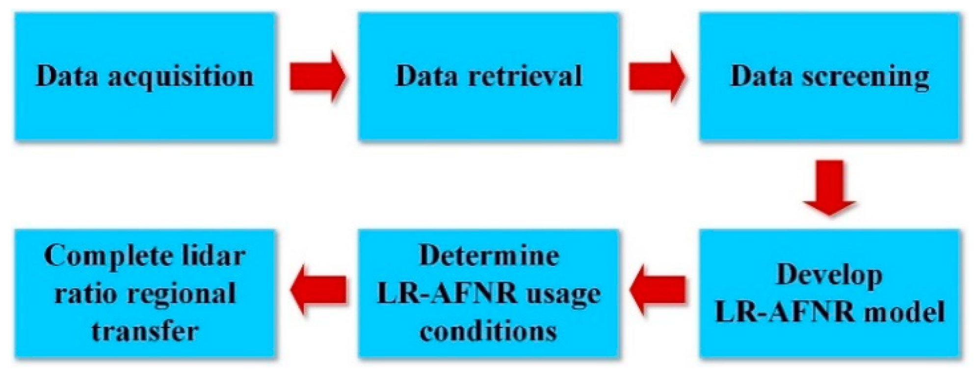
Remotesensing 14 00626 g001
Figure 2. Flowchart of the lidar ratio regional transfer method. The flowchart consists of six steps: data acquisition, data retrieval, data screening, developing the LR-AFNR model, determining the conditions for using the LR-AFNR, and completing the lidar ratio regional transfer.
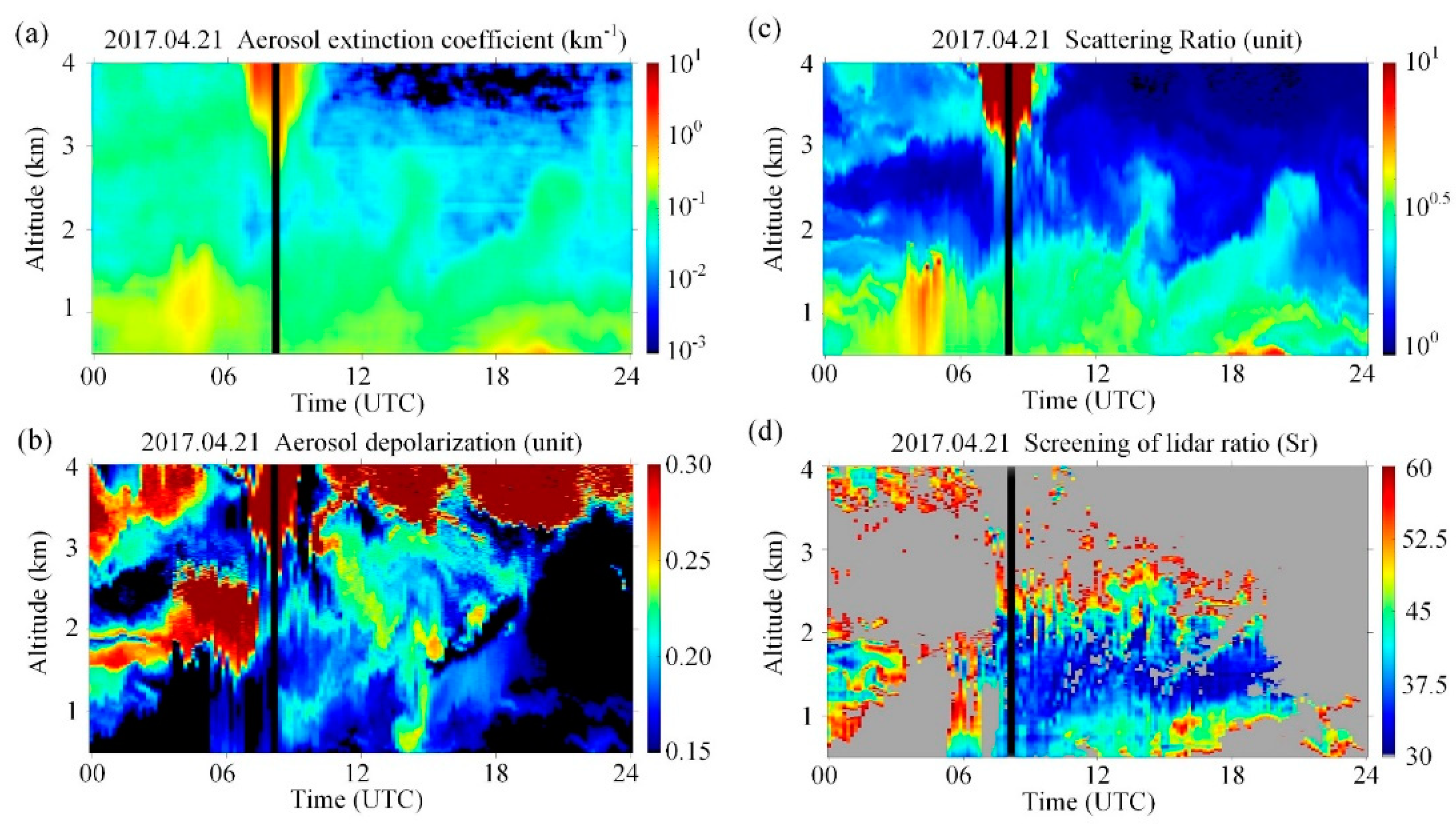
Remotesensing 14 00626 g002
Figure 3. The screening results of dust-dominated observations with the lidar ratio at the KORUS site based on HSRL on 21 April 2017. (a) Aerosol extinction coefficient; (b) Scattering ratio; (c) Aerosol depolarization ratio; (d) Selection of dust-dominated lidar ratio result by screening criteria (grey represents the screened part).
Remotesensing 14 00626 g003
Figure 4. Statistics of the monthly average fraction of relevant absorbing aerosols at the three sites in the selected period. (a) The monthly average fraction distribution of dust, carbonaceous aerosol, and other aerosols at the Yonsei University site in March and April each year from 2016 to 2018; (b) The monthly average fraction distribution of dust, carbonaceous aerosol, and other aerosols at the Cart site from July to October of each year from 2016 to 2018.
Remotesensing 14 00626 g004
Figure 5. Scatter plot of the absorbing aerosol lidar ratio retrieved by HSRL and fraction retrieval by the sun photometer. N and R2 represent the number of fitting points and coefficient of determination, respectively. (ac) represent the fitting relationship of the lidar ratio and dust fraction at the SGP, KORUS, and Madison sites, respectively. The solid red line represents the fitting results, and the color bar represents the dust absorbing mixing ratio; (df) represent the fitting relationship of the lidar ratio and carbonaceous aerosol fraction at the SGP, KORUS, and Madison site, respectively. The solid black line represents the fitting results, and the color bar represents the carbonaceous aerosol absorbing mixing ratio. The top of the subplot represents the equation of the fitted curve.
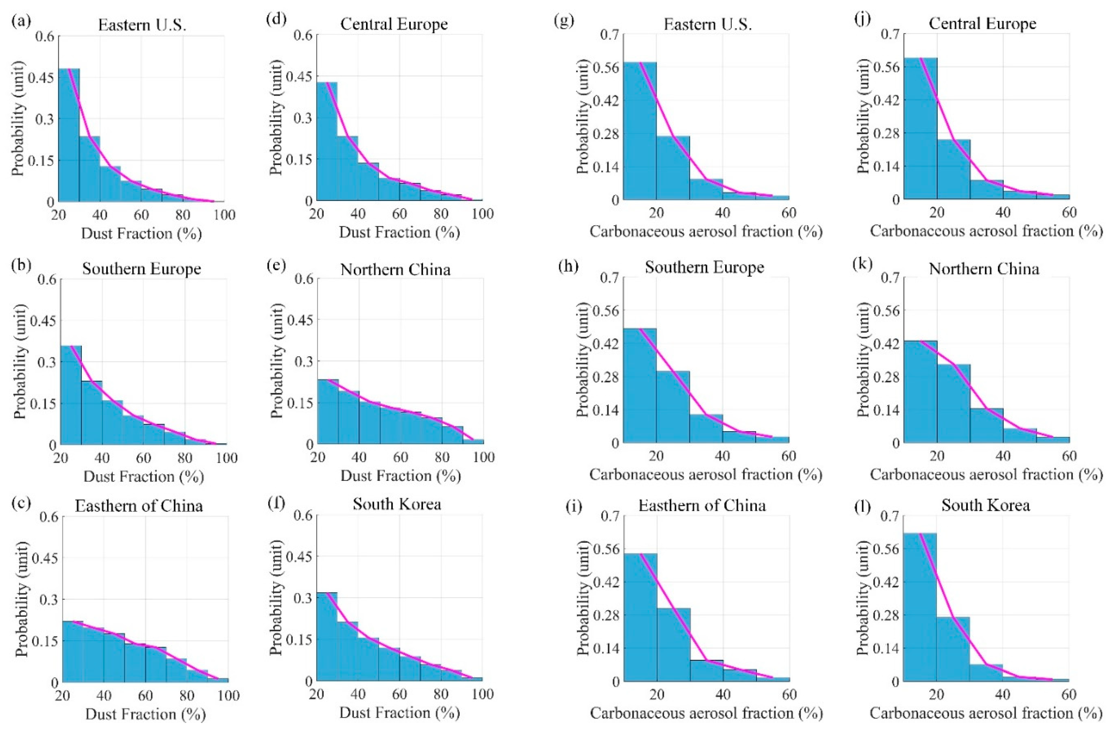
Remotesensing 14 00626 g005
Figure 6. The probability distribution of dust and carbonaceous aerosol fractions in six regions (eastern U.S., central Europe, southern Europe, northern China, eastern China, and South Korea). (af) represent the probability distribution of the dust fraction in the six respective regions; (gl) represent the probability distribution of the carbonaceous aerosol fraction in the six respective regions, where the horizontal coordinate (10–20% of the scale) actually includes only 15–20% of the fraction.
Remotesensing 14 00626 g006
Figure 7. The scatter-fitting relationship between the relative distance and the relative error of the lidar ratio under different aerosol absorbing conditions. The six different scatter colors represent the lidar ratio average relative error between any two sites in the six regions of the eastern US, northern Europe, northern Europe, northern China, eastern China, and South Korea. The solid black line represents the fitting curve, and N and R2 represent the total number of fitting points and the coefficient of determination for the six regions, respectively. (a) Under the condition of heavy dust, point A represents the intersection of the lidar ratio relative error of 23.7% and the relative distance of 108 km; (b) Under the condition of light dust; (c) Under the condition of heavy carbonaceous aerosols, point B represents the intersection of the lidar ratio relative error of 22.9% and the relative distance of 85 km; (d) Under the condition of light carbonaceous aerosols. The dashed line in the subplot points to the equation of the fitted curve.
Remotesensing 14 00626 g007
Figure 8. Take dust as an example, the Klett–Fernald method was used to retrieve the α a , as well as the relative error distribution of α a . (a) The results of α a retrieval using 50 simulated signal profiles in the 3 km boundary layer. The dotted black line (①), the solid blue line (②), the solid purple line (③), and the solid orange line (④) represent the simulated actual α a (the lidar ratio was 56.8 Sr) and the average of α a retrieval after substituting three reference lidar ratios (lidar ratios of 60, 45, and 30 Sr). The three error bars represent the standard deviation of α a retrieval using the three reference lidar ratios (b) Relative error profile of α a retrieval using three reference lidar ratios.
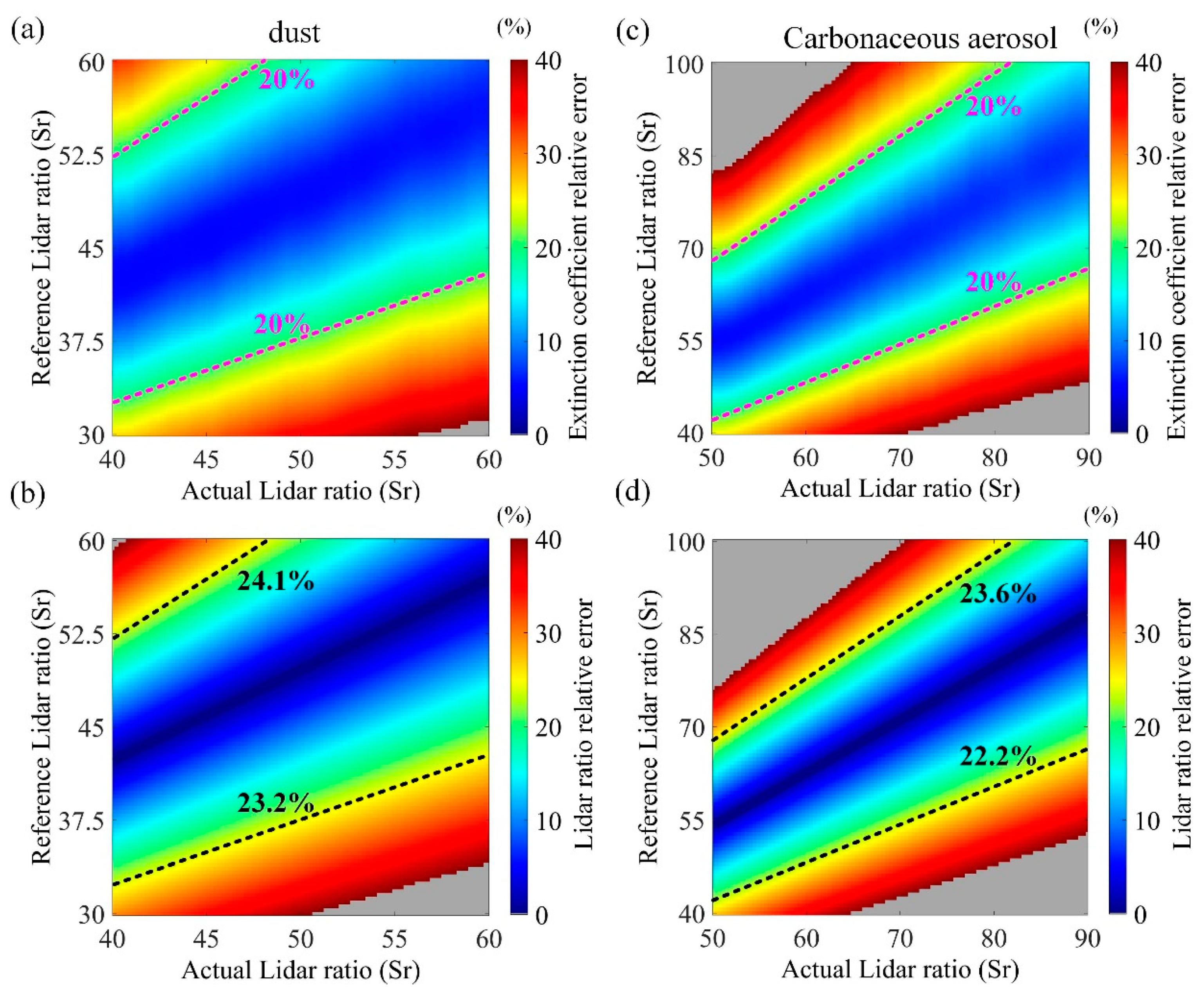
Remotesensing 14 00626 g008
Figure 9. The relationship between the relative error of α a and the lidar ratio, as well as the actual lidar ratio and the reference lidar ratio. (a,b) represent the relative error of α a and the lidar ratio under the dust condition; (c,d) represent the relative error of α a and the lidar ratio under the carbonaceous aerosol condition. The pink dotted line represents the position where the relative error of α a was 20%, and the black dotted line represents the relative error of the lidar ratio at the same position (same horizontal and vertical coordinates) as the pink dotted line in the figure. The grey area represents the part that exceeded the upper limit of the color bar.
Remotesensing 14 00626 g009
Figure 10. 
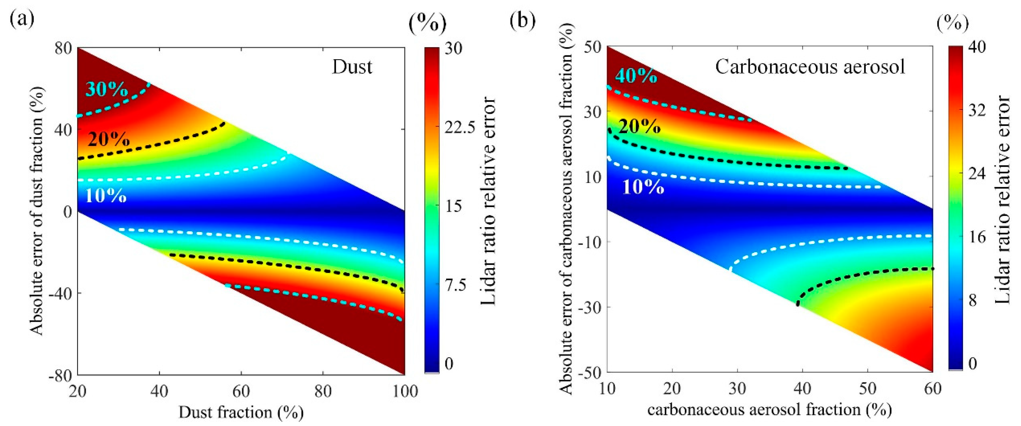
The relationship between the two absorbing aerosol fractions and the lidar ratio relative error. The horizontal and vertical coordinates represent the actual value of the two absorbing aerosol fractions and the absolute error of the reference value, respectively. The color bar represents the relative error of the lidar ratio calculated after the two absorbing aerosol fractions were input into the LR-AFNR. The white part in the figure represents no data. (a) Under the condition of dust, the sky blue, black, and white dotted lines represent the positions where the relative error of the lidar ratio was 30%, 20%, and 10%, respectively; (b) Under the condition of carbonaceous aerosol, the sky blue, black and white dotted lines represent the positions where the relative error of the lidar ratio was 40%, 20%, and 10%, respectively.
Remotesensing 14 00626 g010
Figure 11. The influence of different types of carbonaceous aerosols (different AAEs and SSAs) on the fitting results of the LR-AFNR model. (a,b) represent the results of the fitting curves for different types of carbonaceous aerosols (fresh and aged) under dust-dominated conditions compared with the original fitting curve in Figure 5b. The solid red line represents the original fitting curve, and the black dotted lines represent the fitting curves of fresh and aged smoke; (c,d) represent the results of the fitting curves for different types of carbonaceous aerosols (fresh and aged) under carbonaceous aerosol-dominated conditions compared with the original fitting curve in Figure 5f. The solid black line represents the original fitting curve, and the blue dotted lines represent the fitting curves of fresh and aged smoke. N and R2 represent the number of fitting points and the coefficient of determination, respectively. It should be noted that the solid red line corresponds to the dust fraction range of 20–100% in Figure 5b, and the solid black line corresponds to the carbonaceous aerosol fraction range of 15–60% in Figure 5f, so only part of the curve is shown in this Figure.
Remotesensing 14 00626 g011
Table 1. The information of UW-HSRL sites, which includes the site name, system name, longitude, latitude, and data selection period.
Site NameSystem NameLatitude (°)Longitude (°)Selection Period
SGPBagoHSRL36.62 N97.49 WJanuary 2015–October 2017
KORUSAHSRL37.56 N126.95 EJanuary 2016–December 2018
MadisonBagoHSRL43.01 N89.41 WNovember 2012–June 2019
Table 2. The screening criteria for the lidar ratio data when dust or carbonaceous aerosols are the dominant type.
Dust-Dominated DataCarbonaceous Aerosol-Dominated Data
Height (km)0.5–40.5–4
Aerosol depolarization ratio (unit)0.15–0.30.05–0.15
Scattering ratio (unit)1.2–101.2–10
Lidar ratio (Sr)30–6040–100
Absorbing mixing ratio (%)50–100 (dust)50–100 (carbonaceous aerosol)
Scattering ratio above 4 km (unit) T t   <   R   <   T p T t   <   R   <   T p
Table 3. The information of AERONET sites, which includes the site name, location, longitude, latitude, and data selection period.
Site NameLocationLatitude (°)Longitude (°)Selection Period
CartOklahoma, United States36.61 N97.49 WJanuary 2015–December 2018
Yonsei UniversitySeoul, South Korea37.56 N126.94 EJanuary 2016–December 2018
U of Wisconsin SSECWisconsin, United States43.01 N89.41 WNovember 2012–June 2019
Table 4. The values of AAE and SSA used for fresh and aged smoke conditions for BC and BrC.
BCBrC
Fresh smoke dominated
AAE10.4954.095
AAE20.7650
SSA0.150.85
Aged smoke dominated
AAE10.6055.005
AAE20.9350
SSA0.30.95
Publisher’s Note: MDPI stays neutral with regard to jurisdictional claims in published maps and institutional affiliations.

