Evaluating the Potential of Different Evapotranspiration Datasets for Distributed Hydrological Model Calibration

Abstract

Evapotranspiration (ET), a key component of the hydrological cycle, has a direct impact on runoff and water balance. Various global satellite-based and numerical datasets provide continuous and high spatiotemporal resolution data, which makes it possible to calibrate hydrological parameters against ET. However, the accuracy of ET datasets varies with region and algorithm, introducing uncertainties in hydrological parameter calibration. This study focused on evaluating the potential of different ET datasets in the calibration of distributed hydrological model parameters. Five different ET datasets (PML, SEBAL, EB-ET, GLASS, REA-ET) were evaluated using the water balance method to explore the effect of intrinsic dataset accuracy on applications. The benchmark calibration scheme calibrated parameters by using observed streamflow data from the outlet. Two calibration schemes were proposed to take advantage of the temporal dynamics and spatial patterns of the raw ET datasets. The results show that the model parameters calibrated by all selected ET datasets produced satisfactory results in streamflow simulations. These results were dependent on the calibration schemes and accuracy of ET datasets. Overall, the scheme calibrated by using temporal dynamics of ET at the grid scale provided better streamflow simulations at the basin outlet than the scheme calibrated by using spatial patterns of ET at the basin scale. Three metrics (bias, root mean square error [RMSE], and correlation coefficient [R]) showed that there is a high potential for selected ET datasets to improve soil moisture simulations, as compared to the benchmark scheme. Parameters calibrated by EB-ET and PML datasets provided the best performance in the simulation of streamflow at the outlet and the sub-basin scale. The calibration case with the SEBAL dataset showed the highest potential to improve soil moisture simulation. The annual average ET estimates of these three datasets were closest to the water balance-based ET values.

1. Introduction

Distributed hydrological models, which provide spatial variations in catchment characteristics, are important tools for hydrological forecasting and water resource management [1,2,3]. Accurate forcing data and appropriate parameterization are key factors that enable hydrological models to produce reliable simulations [4]. Traditionally, easy access and high-quality observed streamflow datasets from basin outlets have been used to constrain parameters for hydrological model calibration [5,6]. This method may be reliable in small watersheds with available datasets, but not for large and heterogeneous basins, especially in ungauged basins [6,7,8,9].

In the past 10 years, satellite remote-sensing observations and reanalysis datasets have been frequently applied in model calibrations [10,11,12]. They can provide valuable information about hydrology-relevant variables at increasingly finer spatial and temporal resolutions, including precipitation, total water storage, evapotranspiration (ET), snow cover, and surface soil moisture [13,14,15,16]. Compared with in situ observations at a point scale, remote-sensing observations complement the data at a large regional scale, especially in poorly gauged or ungauged basins.

Evapotranspiration, which entails vegetation transpiration, soil evaporation, and canopy rainfall interception, is a link among water, energy, and carbon cycles and plays an important part in agriculture, water resource management, and climate change [17,18]. As one of the critical components of the hydrological cycle, the accuracy of ET simulations in hydrological models is also a key factor in determining the performance of soil moisture and runoff estimates [19]. Recently, several global ET datasets have been generated by remote-sensing models, and they differ in algorithms, inputs, and parameters [20]. Merging multiple single datasets is also a popular method for generating long-term and large-scale ET datasets [21]. With increasing spatiotemporal resolution and accuracy, gridded satellite-based and merged datasets can provide global and long time series ET estimations, which makes their utilization in hydrological applications possible, especially in poorly gauged regions [22,23,24,25].

Many previous studies have used ET datasets in model calibration and obtained satisfactory results from hydrological simulations. Zhang, et al. [19] used parameters calibrated solely against remote-sensing ET data to estimate runoff series and obtain encouraging monthly and mean annual runoff results in the wetter catchments. Demirel, et al. [26] proposed a novel bias-insensitive spatial pattern metric to utilize satellite observed spatial patterns of ET for model calibration. Dembele, et al. [27] improved the performance of terrestrial water storage and spatial patterns of soil moisture simulations by using multi-variable calibration strategies. However, recent studies have focused more on improving the calibration strategies and frameworks through multi-variable or multi-objective calibration that combines multiple satellite datasets [28,29,30]. Most of the studies use only one dataset and with different calibration schemes to achieve accurate simulation performance. They rarely compare the potential of different ET datasets in model parameter calibration [27], which is important for selecting appropriate ET datasets for hydrological model parameter calibration and algorithms to improve the accuracy of ET datasets. Furthermore, current research mainly concentrates on whether parameters calibrated by ET datasets are suitable for streamflow simulation but rarely evaluate their performance in soil moisture simulations. As an important hydro-meteorological variable and output of the distributed hydrological model [31,32], accurate simulation of soil moisture is also critical in hydrological models for applications, but there is no consistent conclusion as to which parameter calibration method (parameters calibrated by streamflow or calibrated by ET) is more suitable for soil moisture simulation. Thus, the potential of different ET datasets in distributed hydrological model calibrations requires further evaluation with a large amount of observed data.

The overall goal of this study was to investigate the potential of ET datasets, which are generated by different remote-sensing models and algorithms, in model parameter calibration to simulate streamflow and soil moisture. Two calibration schemes considering the temporal dynamics and spatial patterns of ET were proposed in this paper to make full use of information from the raw datasets. The accuracy of ET datasets was quantified by the water balance method [33], and the influence of the relative error of ET datasets on parameter calibration was analyzed. The observed streamflow data were also used to calibrate the parameters as a benchmark to compare with the calibration strategies against ET datasets. The research was conducted in the Ganjiang River Basin (GRB), located in the southern part of China, with sufficient in situ observations, using the variable infiltration capacity (VIC) model during 2003–2014.

2. Study Area and Datasets

2.1. Study Area

The GRB is the seventh-largest branch of the Yangtze River and the largest river in Jiangxi Province in China (Figure 1e). The drainage area is approximately 80,860 km² above the Waizhou hydrological station. The elevation of the GRB (Figure 1a) ranges from 31 to 1183 m above sea level. The GRB has a subtropical humid monsoon climate, with an average annual air temperature of 17.8 °C and approximately 1400–1800 mm of precipitation per year. The heaviest rainfall occurs during the plum rain season between April and June, while monsoon and typhoon rainstorms frequently occur between July and September [34]. Land cover (Figure 1b) is dominated by woodland and wooded grassland, covering approximately 52% and 36% of the GRB, respectively. Approximately 8% of the basin area is cropland concentrated downstream.

2.2. Datasets

2.2.1. Meteorological Data

The meteorological data used to set up the VIC hydrological model included precipitation, air temperature, shortwave radiation, longwave radiation, vapor pressure, wind speed, and atmospheric pressure. The meteorological data from meteorological stations (Figure 1b) within and around the GRB were provided by the National Meteorological Science Data Center (http://data.cma.cn, accessed on 8 October 2021). All meteorological data used in this study are available for the period of 2003 to 2014. They were interpolated into 0.05° grid cells using the inverse distance weighted interpolation algorithm.

2.2.2. Observed Streamflow and Soil Moisture Data

The daily streamflow and in situ soil moisture data are available from the Information Center (Hydrological Monitor and Forecast Center), Ministry of Water Resources of the People’s Republic of China. Figure 1a shows the distribution of 26 hydrological stations, the numbers of which are sorted according to drainage areas of sub-basins (the drainage area of hydrological station No.1 is the largest in the GRB). More details about the hydrological stations are presented in

Table 1. Summary of 26 hydrological stations.

ID	Name	Lat (°)	Lon (°)	Drainage Area (km2)	Timespan
1	Waizhou	28.63	115.83	80,860	1980–2014
2	Zhangshu	28.07	115.53	71,190	1998–2014
3	Xiajiang	27.55	115.15	62,690	1980–2014
4	Ji’an	27.10	114.98	56,180	1980–2014
5	Dongbei	26.57	114.70	40,190	1980–2014
6	Xiashan	25.92	115.22	15,940	1980–2014
7	Julongtan	25.82	115.12	7742	1980–2014
8	Bashang	25.82	114.85	7457	1980–2014
9	Fenkeng	26.13	115.67	6358	1980–2014
10	Gan’an	28.42	115.37	6062	1991–2014
11	Shangshalan	26.93	114.80	5258	1980–2014
12	Shanggao	28.23	114.92	3706	1986–2014
13	Xintian	27.20	115.28	3546	1980–2014
14	Tiantou	25.78	114.65	3196	1980–2014
15	Saikuang	27.18	114.77	3071	1980–2014
16	Hanlinqiao	26.05	115.20	2659	1980–2014
17	Ningdu	26.48	116.02	2286	1980–2014
18	Mazhou	25.52	115.78	1742	1980–2014
19	Linkeng	26.67	114.60	993	1980–2014
20	Weifang	28.13	114.40	975	1980–2014
21	Shicheng	26.37	116.37	659	1980–2014
22	Yangxinjiang	25.32	115.38	561	1980–2014
23	Junmenling	25.23	115.75	455	1984–2014
24	Dutou	24.78	114.63	434	1980–2014
25	Luxi	27.63	114.03	330	1980–2014
26	Chuzhou	26.35	114.13	287	1980–2014

. Figure 1c shows the distribution of 28 soil moisture stations in the GRB, and

Table 2. Summary of 28 soil moisture stations.

ID	Name	Lat (°N)	Lon (°E)	Land Use	Soil Texture of the First Layer	Soil Texture of the Second Layer	Timespan
1	57992	25.68	114.78	Wooded grassland	Clay loam	Clay loam	2013–2014
2	623A1600	27.83	115.03	Cropland	Clay	Clay	2011–2014
3	623A1700	25.73	114.73	Wooded grassland	Clay loam	Clay loam	2011–2014
4	623A1800	25.28	114.93	Wooded grassland	Clay loam	Clay	2011–2014
5	623A1900	25.83	115.13	Wooded grassland	Clay loam	Clay loam	2011–2012
6	623A2100	26.58	115.38	Woodland	Clay loam	Clay	2011–2012
7	623A2200	24.78	114.48	Woodland	Clay loam	Clay	2011–2012
8	623A2500	26.13	116.18	Woodland	Clay loam	Clay	2011–2012
9	623A2600	26.08	115.58	Grassland	Clay loam	Clay loam	2011–2012
10	623A2700	25.53	115.78	Cropland	Clay loam	Clay loam	2011–2014
11	623A2800	27.33	115.13	Grassland	Clay	Clay	2011–2013
12	623A2900	26.58	114.73	Woodland	Clay	Clay	2011–2012
13	623A3100	26.38	114.58	Cropland	Clay	Clay	2012–2013
14	623A3200	27.08	115.63	Wooded grassland	Clay loam	Clay	2011–2014
15	623A3300	26.68	114.68	Cropland	Clay	Clay	2012–2014
16	623A3500	27.38	114.58	Woodland	Clay	Clay	2011–2013
17	623A3600	27.03	114.33	Wooded grassland	Clay loam	Clay	2011–2013
18	623A3900	27.13	114.93	Cropland	Clay	Clay	2011–2012
19	623A4000	28.13	114.48	Wooded grassland	Clay loam	Clay	2011–2014
20	623A4300	27.33	114.48	Woodland	Clay loam	Clay	2011–2012
21	623A5100	28.18	115.63	Cropland	Clay	Clay	2011–2012
22	623A5300	28.38	115.43	Cropland	Clay	Clay	2011–2014
23	623A5700	28.08	115.33	Cropland	Clay loam	Clay	2012–2014
24	623A5900	27.88	114.78	Wooded grassland	Clay	Clay	2012–2013
25	623A6100	27.33	115.73	Grassland	Clay loam	Clay	2011–2014
26	J7258	27.13	113.98	Woodland	Clay loam	Clay	2013–2014
27	J8248	26.83	114.93	Wooded grassland	Clay	Clay	2013–2014
28	J9901	26.43	115.98	Wooded grassland	Clay loam	Clay loam	2013–2014

shows the details of each station. The in situ soil moisture datasets represent three different depths of soil layers (10, 20, and 40 cm). For a better comparison with the simulated soil moisture of the VIC model, the in situ soil moisture was integrated to 0–40 cm and converted to volumetric water content. Sufficient in situ datasets are helpful for evaluating the performance of calibration schemes against ET datasets in hydrological models. Figure 1c,d show the soil texture of two layers (0–30 cm and 30–100 cm). Soil parameters of the VIC model were defined from a soil texture map provided by Reynolds, et al. [35].

2.2.3. Gridded Evapotranspiration (ET) Datasets

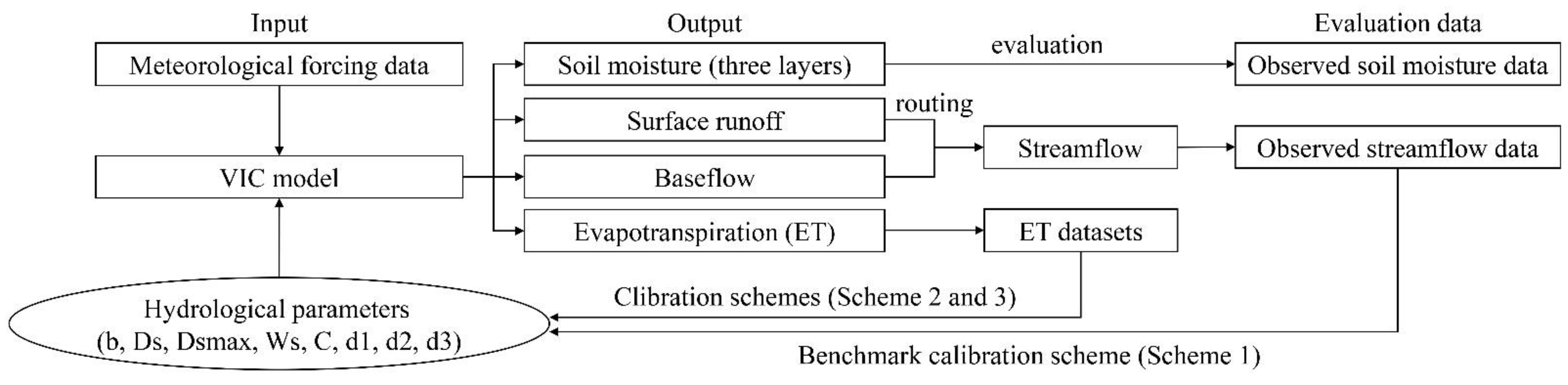
A total of five gridded ET datasets were used in this study, including four satellite-based ET datasets (PML, SEBAL, EB-ET, and GLASS) and one merged dataset (REA-ET). The algorithms used in each of these ET datasets were different, including the Penman–Monteith–Leuning (PML) model, models based on surface energy balance (SEBAL and EB-ET), and multi-model ensemble method (GLASS). Furthermore, the REA-ET dataset differs from other models in that it uses the reliability ensemble averaging (REA) method to merge three reanalysis datasets (ERA5, GLDAS2, and MERRA2). The merged dataset was found to be significantly improved compared with the three individual selected datasets [21]. A summary of five gridded ET datasets is provided in

Table 3. Summary of ET datasets.

Dataset	Method	Resolution		Reference/Data Portal	Timespan	Spatial Coverage
		Spatial	Temporal
PML	PML	0.05°	8d	Zhang, et al. [36] https://data.tpdc.ac.cn/en/data/48c16a8d-d307-4973-abab-972e9449627c/, accessed on 25 October 2021.	2002–2019	Global
SEBAL	SEBAL	1km	daily	Cheng, et al. [37] https://zenodo.org/record/4243988, accessed on 25 October 2021.	2001–2018	China
EB-ET	SEBS	5km	daily	Chen, et al. [38] https://data.tpdc.ac.cn/en/data/df4005fb-9449-4760-8e8a-09727df9fe36, accessed on 25 October 2021.	2000–2017	Global
GLASS	MOD16, RRS-PM, P-T, MS-PT, UMD-SEMI	1km	8d	Liang, et al. [39] http://www.glass.umd.edu/, accessed on 25 October 2021.	2000–present	Global
REA-ET	Merged dataset (ERA5, MERRA2, GLDAS)	0.25°	daily	Lu, Wang, Chen, Li, Hagan, Kattel, Peng, Jiang and Su [21] https://zenodo.org/record/4595941, accessed on 25 October 2021.	1980–2017	Global

Note: PML: Penman–Monteith–Leuning; SEBAL: Surface Energy Balance Algorithm of Land; SEBS: Surface Energy Balance System; EB-ET: the surface energy balance based global land evapotranspiration; GLASS: the global land surface satellite product; REA: the reliability ensemble averaging; MOD16: MODIS ET dataset algorithm; RRS-PM: revised remote sensing-based Penman-Monteith ET algorithm; MS-PT: modified satellite-based Priestley-Taylor ET algorithm; UMD-SEMI: semi-empirical Penman ET algorithm of the University of Maryland; ERA5: the fifth-generation ECMWF Re-Analysis [40]; MERRA2: the second Modern-Era Retrospective analysis for Research and Applications [41]; GLDAS: Global Land Data Assimilation System ET [42].

, and more information on each dataset can be found in the corresponding references.

For a fair comparison, all gridded ET datasets were calculated on an 8-day timescale and rescaled to a 0.05° spatial scale to maintain consistent spatiotemporal resolution. Spatial patterns of annual average ET for the five selected ET datasets are shown in Figure 2. SEBAL and EB-ET had similar spatial distributions of annual average ET. It is likely that they are based on the surface energy balance algorithm. PML and GLASS show that ET is higher in the upstream region of GRB, while ET from REA-ET dataset is higher in the downstream and middle regions of the GRB.

3. Methodology

3.1. Hydrological Model

The VIC model [43,44] is a large-scale distributed hydrological model based on soil vegetation atmospheric transfer schemes, which can simulate the land surface energy and water balance in each grid cell. The VIC model has been widely applied to simulate surface runoff, baseflow, ET, and soil moisture dynamics for further data construction, evaluation, assimilation, and forecasting studies [45,46,47]. The VIC model estimates ET as the sum of three components: canopy layer evaporation (Ec), vegetation transpiration (Et), and evaporation from the bare soil surface (Es). Soil moisture was estimated using three distinct soil layer schemes. The Rosenbrock algorithm [48] was used in this study to calibrate eight hydrological parameters, which needed to be optimized in the VIC model. The introduction of calibrated parameters is provided in

Table 4. Hydrological parameters in the VIC model for calibration.

Parameter	Unit	Description	Feasible Range
			Minimum	Maximum
b	-	variable infiltration curve parameter	0.0001	0.35
Ds	-	fraction of Dsmax where non-linear baseflow begins	0.0001	0.4
Dsmax	mm	maximum velocity of baseflow	0.0	40.0
Ws	-	fraction of maximum soil moisture where non-linear baseflow occurs	0.4	1.0
C	-	exponent of the nonlinear part of the baseflow curve	2.0	2.0
d1	m	thickness of first soil moisture layer	0.1	0.1
d2	m	thickness of second soil moisture layer	0.1	1.5
d3	m	thickness of third soil moisture layer	0.1	1.5

. More details on the VIC model setup and the feasible range of parameters can be found in the previous work of Wu, et al. [49]. A large-scale routing model developed by Lu, et al. [50] was used for routing the total grid-generated runoff through the river network. In this study, a daily VIC model with a spatial resolution of 0.05° was used for the GRB. A flow chart of the VIC model and calibration schemes is shown in Figure 3.

3.2. Model Calibration and Evaluation

The modeling period extended from 2003 to 2014 with 2 years of model warm-up (2003–2004), 6 years for calibration (2005–2010), and 4 years for evaluation (2011–2014). The daily streamflow data from the outlet of the GRB were used for model calibration and evaluation. The streamflow datasets from the other 25 hydrological stations and in situ soil moisture datasets were used for model evaluation.

3.2.1. Calibration on Streamflow Data—Benchmark Scheme

The benchmark calibration scheme (Scheme 1) constrained parameters by using observed streamflow data from the outlet of the GRB. The objective function Equation (1) for Scheme 1 is obtained by maximizing the widely used Nash–Sutcliffe coefficient of efficiency (NSE) between the observed and simulated streamflow.

$$\mathrm{NSE}=1-\frac{{\displaystyle \sum _{i=1}^n{\left(Q_{sim}{}_{,i}-Q_{obs}{}_{,i}\right)}^2}}{{\displaystyle \sum _{i=1}^n{\left(Q_{obs}{}_{,i}-\overline{Q_{obs}}\right)}^2}}$$

(1)

where $Q_{sim}{}_{,i}$ and $Q_{obs}{}_{,i}$ are the simulated and observed streamflow at time step i respectively; $\overline{Q_{obs}}$ is the time-averaged observed streamflow, and n is the number of samples. Moriasi, et al. [51] suggested that model performance for streamflow can be categorized into four classes according to the NSE values: very good (0.75 < NSE ≤ 1.00); good (0.65 < NSE ≤ 0.75); satisfactory (0.50 < NSE ≤ 0.65); and unsatisfactory (NSE ≤ 0.50).

3.2.2. Calibration on ET Dataset

Two calibration schemes for ET (Schemes 2 and 3), each with a different objective function, were proposed in this study. Different schemes were calibrated at different spatial scales; gridded and catchment scales were used for Schemes 2 and 3, respectively. For grid calibration, each grid cell had its own set of hydrological parameter values. For catchment calibration, all grid cells in the GRB had the same set of hydrological parameter values. As the scale increased from the grid to the catchment, the model became more lumped.

Scheme 2 focused on the temporal dynamics of ET and used raw ET datasets for model calibration. The modeled ET was matched with the ET datasets on the time series of each grid cell in the basin, and the objective function Equation (2) was obtained by maximizing the NSE of each grid cell. The gridded ET datasets make it possible for the distributed hydrological model to optimize the parameters at a grid scale.

$${\mathrm{NSE}}_i=1-\frac{{\displaystyle \sum _{j=1}^t{\left(E{T}_{sim}{}_{,j}-E{T}_{obs}{}_{,j}\right)}^2}}{{\displaystyle \sum _{j=1}^t{\left(E{T}_{obs}{}_{,j}-\overline{E{T}_{obs,i}}\right)}^2}}$$

(2)

where $E{T}_{sim}{}_{,j}$ and $E{T}_{obs}{}_{,j}$ are the simulated ET from the VIC model and the observed ET from selected datasets at time step j, respectively; i is the number of each grid cell in the basin, and $\overline{E{T}_{obs,i}}$ is the time-averaged observed ET of one grid cell.

Scheme 3 focused on the spatial patterns of ET because different datasets may give very different absolute values of a specific variable but have fewer uncertainties in the spatial patterns. To eliminate the effects of the magnitude of ET values, a new bias-insensitive metric for spatial pattern representation, called spatial pattern efficiency (SPE), was proposed in our study. The SPE adopted from the efficiency metric of spatial patterns (E_sp) [22] and the spatial efficiency metric (SPAEF) [26] is a multi-component metric that matches with existing metrics. However, the existing metrics E_sp and SPAEF have some limitations in terms of application. When E_sp is applied to a large basin, the mismatching of ET in some grids will cause an abnormally large r_s value in the equation. The number of bins in the SPAEF is defined by users, which may increase human errors. The SPE proposed in this study is defined by Equations (3)–(7), and the optimal value is 1.

$$\mathrm{SPE}=1-\sqrt{{(R-1)}^2+{(\beta -1)}^2+{(\alpha -1)}^2}$$

(3)

$$R=\rho (E{T}_{sim},E{T}_{obs})$$

(4)

$$\beta =\left(\frac{{\sigma }_{sim}}{{\mu }_{sim}}\right)/\left(\frac{{\sigma }_{obs}}{{\mu }_{obs}}\right)$$

(5)

$$\alpha =\mathrm{RMSE}(Z_{E{T}_{sim}},Z_{E{T}_{obs}})$$

(6)

$$\mathrm{RMSE}=\sqrt{\frac{1}{n}{\displaystyle \sum _{i=1}^n{(X_i-Y_i)}^2}}$$

(7)

where R is the Pearson correlation coefficient between the simulated ET ($E{T}_{sim}$) and the observed ET from selected datasets ($E{T}_{obs}$), $\beta$ is the fraction of the coefficient of variations representing spatial variability, $\mu$ and $\sigma$ represent the average and the standard deviation, respectively, and $\alpha$ is the spatial location matching term calculated as the root mean square error (RMSE) of the z-score standardized values of $E{T}_{sim}$ and $E{T}_{obs}$. Each component in the SPE contains different information about spatial patterns, and all these three terms are bias-insensitive. The correlation term R expresses the spatial correlation of ET values, while the coefficient of variation term $\beta$ assesses the similarity in the dispersion of the probability distributions. The spatial location matching term $\alpha$ accounts for correlation or variation.

3.2.3. Model Evaluation Metrics

In this study, five indices including NSE, Kling-Gupta efficiency (KGE) [52], relative error (RE), bias, RMSE, and correlation coefficients (R) were chosen to evaluate the uncertainties and errors in the streamflow and soil moisture simulations. The temporal dynamics of streamflow were evaluated using NSE, KGE, and RE. KGE from Equations (8)–(10) was used to comprehensively evaluate model performance by incorporating correlation, variability, and bias error into a multi-objective criterion in a balanced manner. Compared with KGE, NSE provides a higher streamflow weight and indicates an ability to reproduce middle and high flows.

Bias, RMSE, and R were used to discuss the accuracy of the average, temporal dynamics, and relevance between the simulated and observed soil moisture. R observes the degree of linear correlation, and RMSE is used for the bias evaluation of the temporal dynamics of soil moisture. Additionally, RE (Equation (11)) and bias (Equation (12)) express the comparative values of the two sets of data. Soil moisture has a strong variability owing to the effects of heterogeneous surface conditions and atmospheric forcings [53], which causes a spatial mismatch between the grid-scale simulations and the point-scale observations. Since a station can represent the surrounding area at a small spatial scale [54] and representative errors have no effect on the relative accuracy assessment of different gridded simulations [55], in situ soil moisture observations at a point scale can be used to evaluate simulated results at a grid scale directly.

$$\mathrm{KGE}=1-\sqrt{{(R-1)}^2+{(\beta -1)}^2+{(\gamma -1)}^2}$$

(8)

$$\beta =\frac{{\mu }_{sim}}{{\mu }_{obs}}$$

(9)

$$\gamma =\left(\frac{{\sigma }_{sim}}{{\mu }_{sim}}\right)/\left(\frac{{\sigma }_{obs}}{{\mu }_{obs}}\right)$$

(10)

$$\mathrm{RE}=\frac{{\mu }_{sim}-{\mu }_{obs}}{{\mu }_{obs}}\times 100\%$$

(11)

$$\mathrm{Bias}=\overline{S{M}_{sim}}-\overline{S{M}_{obs}}$$

(12)

where $\beta$ is the fraction of the coefficient of variation representing spatial variability. The $\mu$ and $\sigma$ represent the average and standard deviation, respectively.

3.3. Evaluation Method of ET Datasets

In this study, the water balance method was used to assess different ET datasets at the basin and sub-basin scales. The evaluation was performed over 25 sub-basins and the entire basin on a multi-year (2005–2010) average scale. The water balance-based ET estimates were calculated using the observed precipitation (P), streamflow (Q), and total water storage change (ΔS) in Equation (13). On a multi-year timescale, ΔS can be neglected. The evaluation metric RE was used to compare the annual average ET from various datasets with the water balance-based ET.

$$\mathrm{ET}=P-Q-\Delta S$$

(13)

4. Results

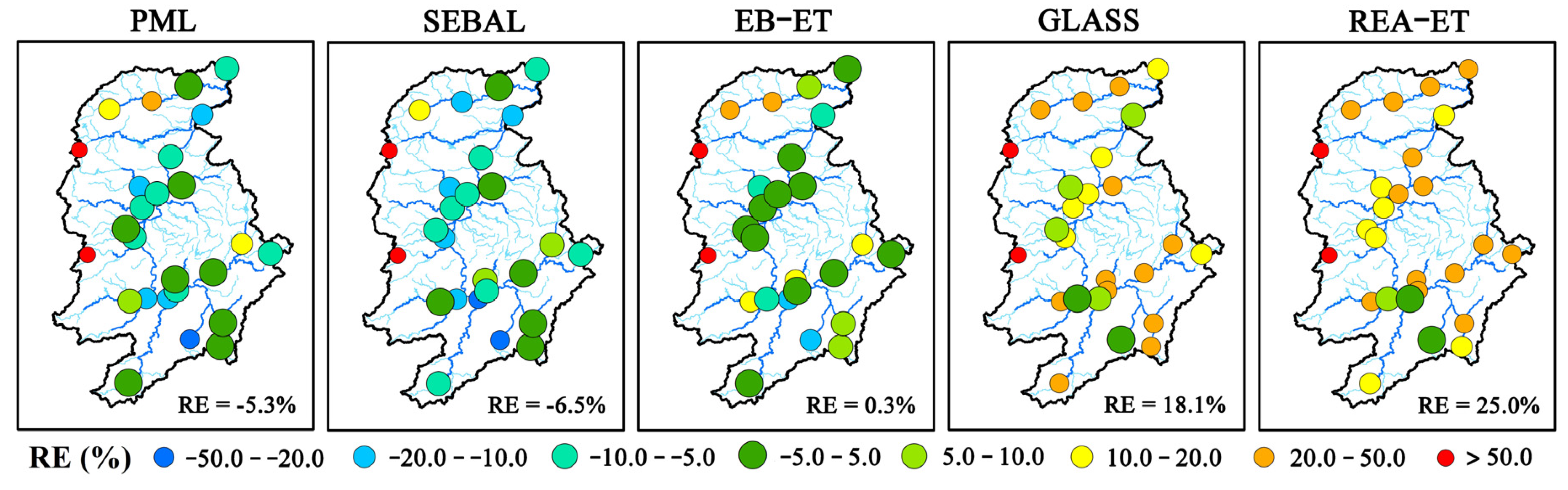
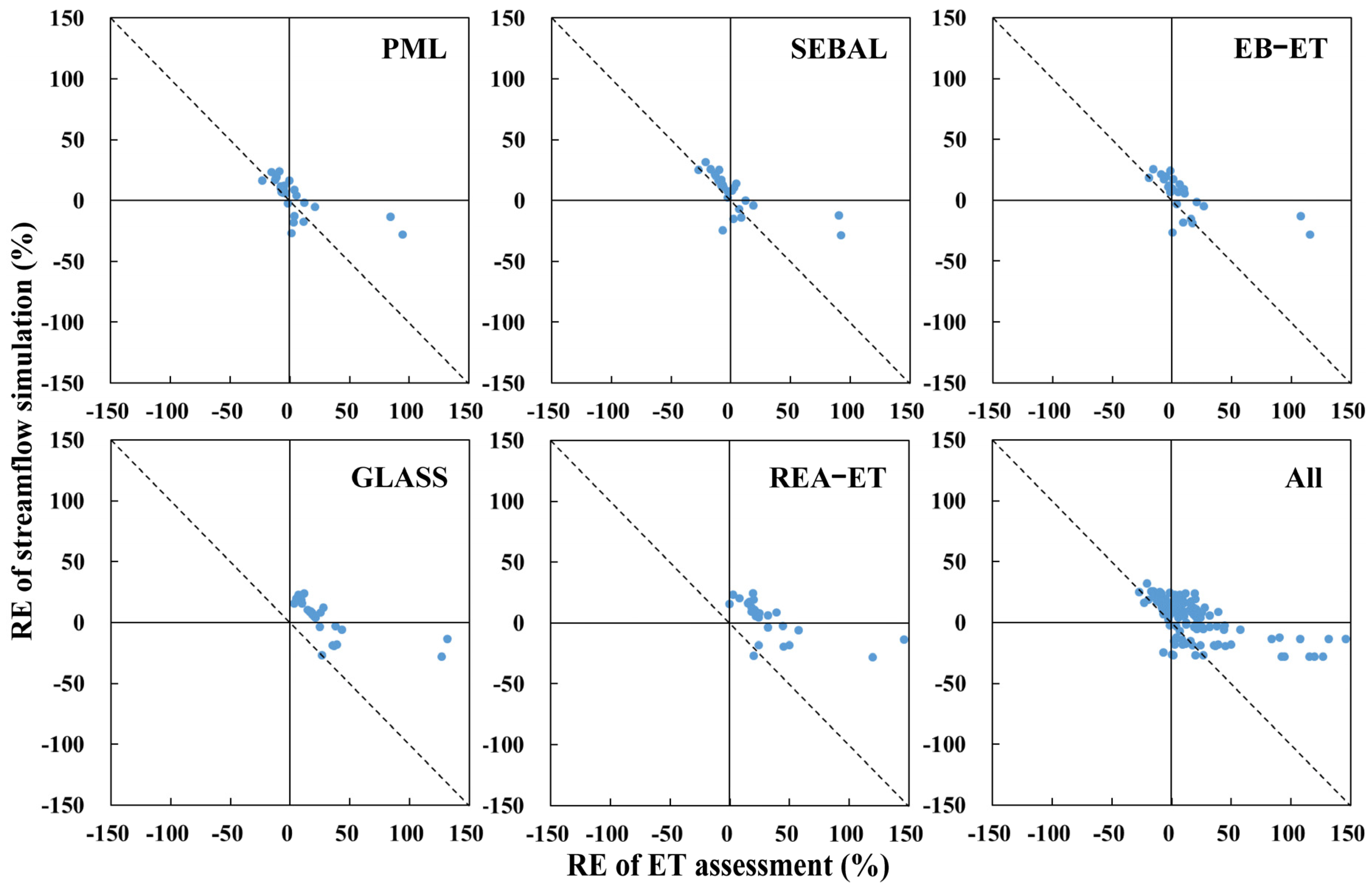
4.1. Assessment of ET Datasets

ET datasets were evaluated using the water balance method with available precipitation and streamflow observations. The distribution of RE between ET datasets and the annual average water balance-based ET is shown in Figure 4. Compared with the water balance-based ET, three datasets (EB-ET, PML, and SEBAL) performed well on annual basin-average ET estimates (the absolute RE was less than 10.0%), while two datasets (GLASS and REA-ET) overestimated the annual basin-average ET with an RE more than 18.0%. EB-ET had the best performance in terms of the annual basin-average ET estimates with minimum absolute RE values (RE = 0.3%).

On the sub-basin scale, three datasets (PML, SEBAL, and EB-ET) had a similar error distribution in the GRB and generally captured the spatial patterns of the annual average ET in large sub-basin regions. Although EB-ET performed well on the basin-average ET estimates, the annual average ET in small sub-basin regions (the drainage area is less than 3000 km²) was unsatisfactory (the absolute RE in 55% of small sub-basins was over 10.0%). Comparatively, REA-ET had the highest ET estimates among the five datasets, with RE in 60% of sub-basins over 20.0%. Similarly, GLASS tended to overestimate ET estimates, with RE in 56% of sub-basins over 20.0%. All datasets overestimated the annual average ET in the two sub-basins above Chuzhou (No. 26) and Luxi (No. 25) hydrological stations, respectively (RE > 50%). The possible reason for ET overestimation is that rescaling ET or precipitation datasets to 0.05° grids in smaller sub-basins (the drainage areas above Chuzhou and Luxi stations are less than 300 km²) will bring more errors [56].

Limited by the number of hydrological stations and evaluation methods, assessment results from the water balance method can only reflect the validity of annual average ET at the basin or sub-basin scales. The accuracy of fine spatial distribution and temporal dynamics of ET datasets cannot be measured in the GRB using existing methods.

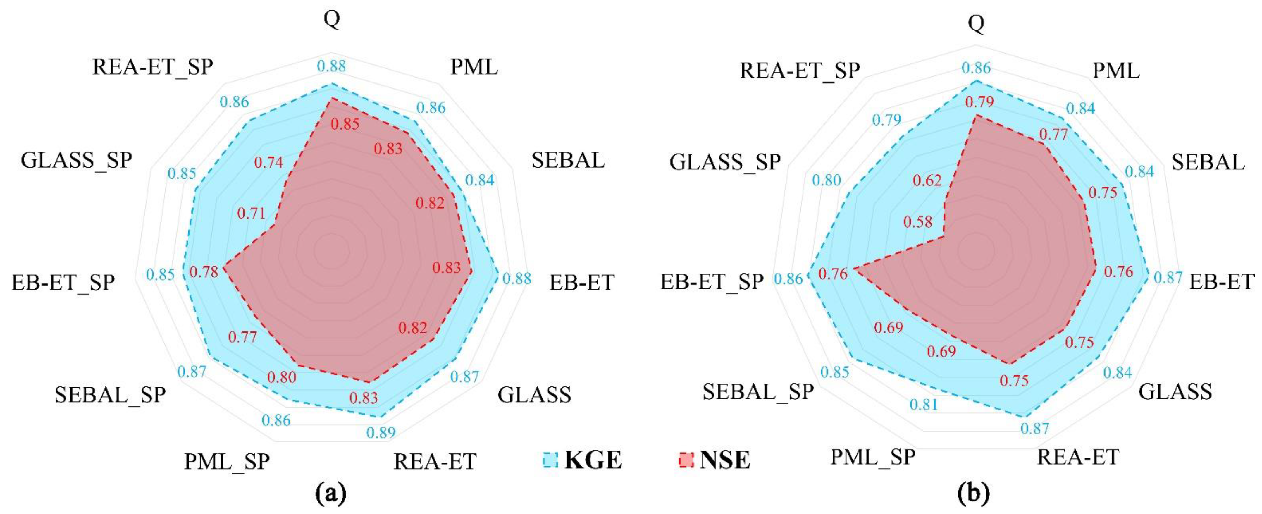
4.2. Model Performance for Streamflow at the Outlet of the Ganjiang River Basin (GRB)

For streamflow at the outlet of the GRB, the model performance for the benchmark calibration scheme (Scheme 1) is shown in Figure 5. The NSE was 0.85 (KGE = 0.88, RE = 9.3%) in the calibration period and 0.79 (KGE = 0.86, RE = 4.3%) during the evaluation period. The benchmark scheme produced “very good” results in terms of the NSE metric (NSE > 0.75), reproducing the temporal dynamics of streamflow during the entire simulation period. The results of Scheme 1 verify that the VIC model can provide a reliable and stable prediction of streamflow in the GRB.

The performance of the two calibration schemes with the five ET datasets is shown in Figure 6. The NSE of each calibration strategy with ET datasets ranged from 0.71 to 0.83 in the calibration period and 0.58 to 0.77 in the evaluation period, corresponding to a decrease compared to that of Scheme 1. As for the KGE, comprehensively evaluating the temporal dynamics of streamflow, the top two best evaporation datasets for the calibration strategy of Scheme 2 were REA-ET (0.89 and 0.87 in the calibration and evaluation periods, respectively) and EB-ET (0.88 and 0.87 in the calibration and evaluation periods, respectively), which performed better than Scheme 1 in the calibration and evaluation periods. EB-ET performed better in Scheme 3 (the KGE was 0.85 and 0.86 in the calibration and evaluation periods, respectively), and was more stable, especially during the evaluation period, followed by the PML and SEBAL datasets.

All datasets used in Scheme 2 had a good effect on streamflow simulation with all cases having an NSE over 0.75 and KGE over 0.84 in the calibration and evaluation periods. The streamflow simulation performance of Scheme 3 was not as good as that of Scheme 2, and the performances of most ET datasets used in Scheme 3 worsened during the evaluation period. Overall, the calibration strategy of Scheme 2 (average NSE = 0.79; average KGE = 0.86) provided better simulated streamflow at the outlet than Scheme 3 (average NSE = 0.64; average KGE = 0.75). Particularly in the evaluation period, Scheme 2 provided a more reliable and stable prediction of streamflow than Scheme 3.

The results of RE in Figure 7 show that most ET datasets performed well in model calibrations, with small relative errors in streamflow simulations as compared with that of the benchmark Scheme 1. The maximum RE was obtained with SEBAL, with the RE approximately 4% higher than that of Scheme 1 in both the calibration and evaluation periods. The PML and EB-ET datasets also provided similar results to Scheme 1, with the RE slightly higher than that of Scheme 1 in the evaluation period. Calibration cases using GLASS and REA-ET datasets had the minimum RE of the streamflow simulations.

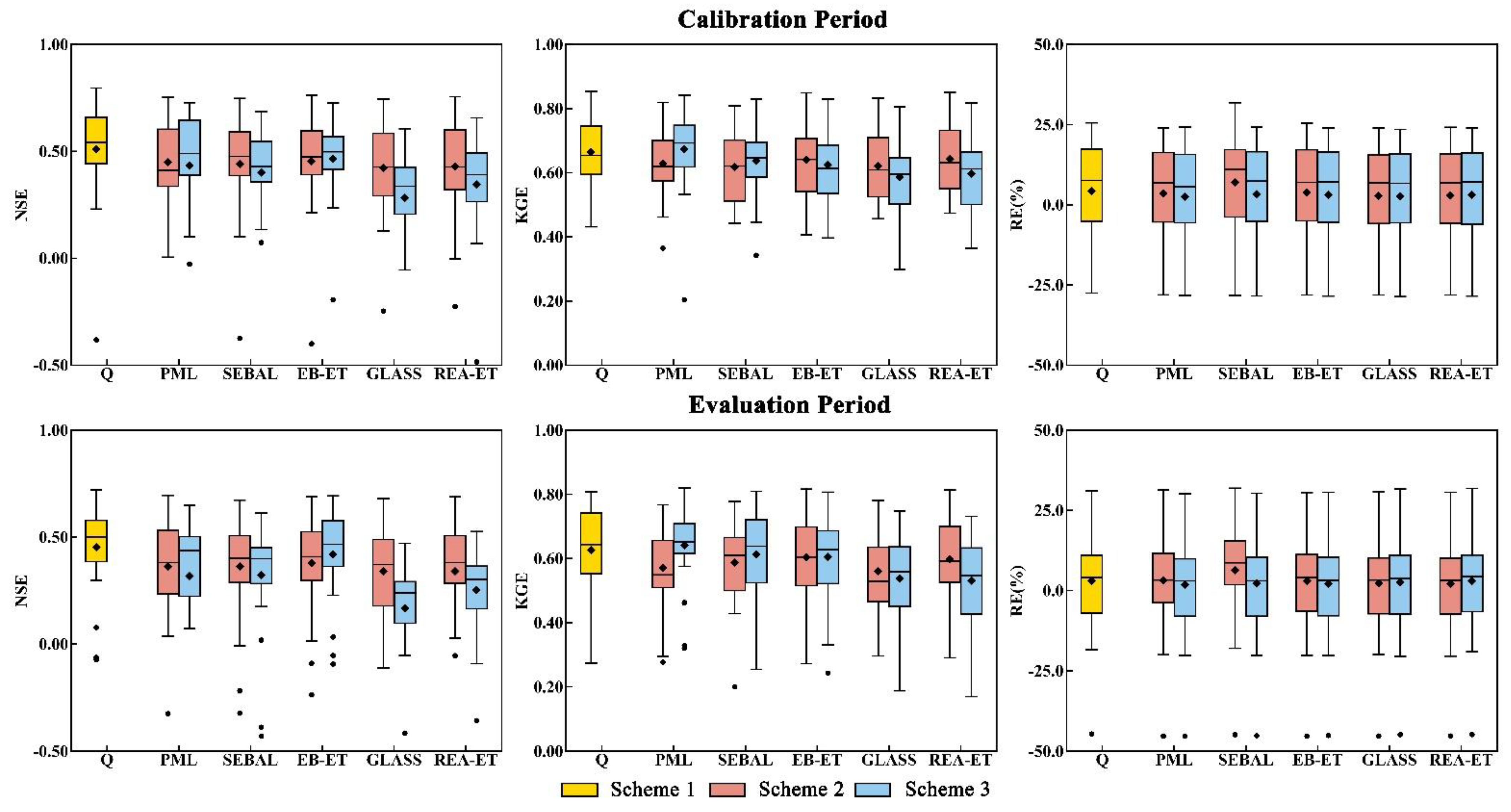
4.3. Model Performance for Streamflow in Sub-Basins

Twenty-five hydrological stations in the GRB were helpful in evaluating the model performance of calibration schemes against different ET datasets at a sub-basin scale. The results of the calibration cases are shown in Figure 8. The performances of schemes calibrated on ET datasets for streamflow in sub-basins are consistent with the results of streamflow at the outlet. The ET datasets used in model calibration, which show a high potential to simulate streamflow at the outlet, can also provide a good performance for sub-basin scale streamflow simulations. For Scheme 2, the highest performances of average NSE and average KGE were obtained with EB-ET (average NSE = 0.45 and 0.38 and average KGE = 0.64 and 0.60 in the calibration and evaluation periods, respectively) and REA-ET (average NSE = 0.43 and 0.34 and average KGE = 0.64 and 0.60 in the calibration and evaluation periods, respectively). EB-ET and PML were the two best evaporation datasets in calibration Scheme 3 for the evaluation metrics of NSE and KGE. EB-ET produced the highest average NSE (average NSE = 0.46 and 0.42 in the calibration and evaluation periods, respectively) of sub-basin scale streamflow simulations, while PML performed better on the average KGE (average KGE = 0.67 and 0.64 in the calibration and evaluation periods, respectively), which was also higher than that of Scheme 1.

The calibration strategy of Scheme 2 had fewer advantages in streamflow simulations at the sub-basin scale than that of Scheme 3, which is different from the results in Section 4.2. For example, the three evaluation metrics of Scheme 3 with PML performed better than those of Scheme 2 in the calibration and evaluation periods. The KGE of Scheme 3 with SEBAL (the average KGE = 0.64 and 0.61 in the calibration and evaluation periods, respectively) was higher than that of Scheme 2 (the average KGE = 0.62 and 0.59 in the calibration and evaluation periods, respectively). The calibrated parameters of Scheme 3 against EB-ET were more stable during the evaluation period than those of Scheme 2. Scheme 2 with GLASS and REA-ET datasets provided better streamflow simulations than Scheme 3, with the average NSE and KGE of Scheme 2 being higher than those of Scheme 3.

The RE of each sub-basin between simulated and observed streamflow, shown in Figure 8, did not show any clear differences in each calibration case; thus, the distribution of RE is shown in Figure 9. The results show that the distribution of RE from different calibration cases is consistent in the GRB, with the simulations tending to underestimate streamflow in the west and overestimate streamflow in the large sub-basins. The GLASS and REA-ET datasets, which had higher annual average ET compared with the water balance-based ET, provided lower simulated streamflow in the large sub-basins compared with the results produced by other ET datasets. The parameters calibrated by the GLASS and REA-ET datasets tend to produce less streamflow in simulations by increasing ET estimations to match the datasets.

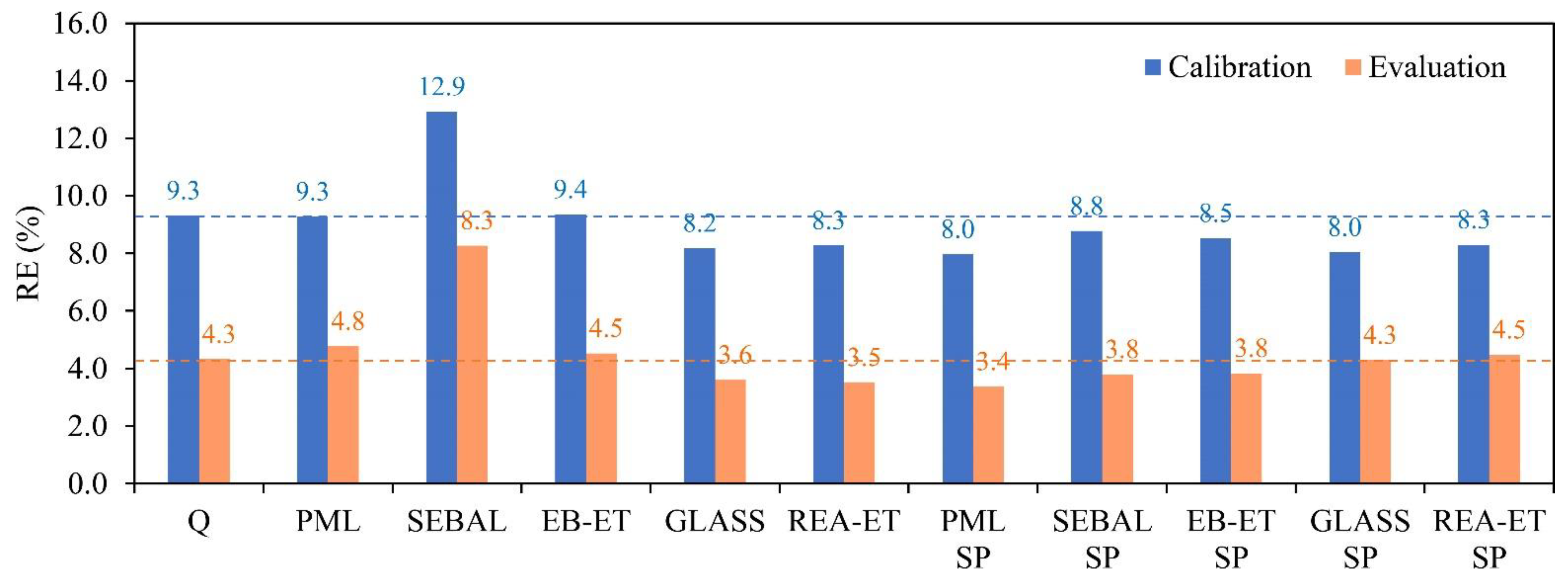
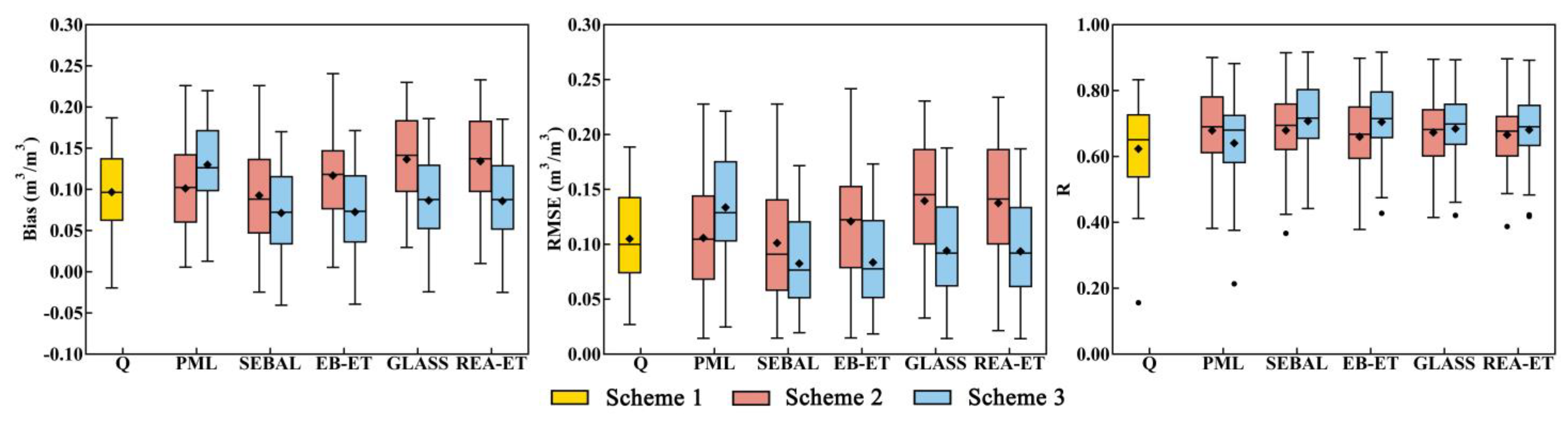
4.4. Model Performance for Soil Moisture

The comparison between the in situ observed soil moisture from 28 stations and the modeled soil moisture is depicted in Figure 10. The time series of soil moisture observations from each station were slightly different, while the overall timespan was 2011–2014. The ET datasets showed a high potential to improve the temporal dynamics of modeled soil moisture with all calibration schemes (the average R of 0–40 cm depth soil moisture simulations from all calibration cases ranged from 0.64 to 0.71), outperforming the benchmark Scheme 1 (average R = 0.62). The evaluation metrics bias and RMSE showed that except PML, the other four datasets used in calibration Scheme 3 can reduce errors in 0–40 cm depth soil moisture simulations from the perspective of average value and temporal dynamics. SEBAL (average bias = 0.08, R = 0.71, and RMSE = 0.08) and EB-ET (average bias = 0.08, R = 0.70, and RMSE = 0.08) were the two best ET datasets among all calibration cases, performing better in 0–40 cm depth soil moisture simulations than Scheme 1 (average bias = 0.10, R = 0.62, and RMSE = 0.10). The overall worst performance was obtained by calibration strategies using GLASS (average bias = 0.14, R = 0.67, and RMSE = 0.14) and REA-ET (average bias = 0.13, R = 0.67, and RMSE = 0.14) datasets. The results of the soil moisture simulations are consistent with the results of ET datasets assessment in Section 4.1.

Using the No. 14 soil moisture station as an example, in which the results from different calibration cases were consistent with the overall outcome, we explored the potential of different calibration schemes using different ET datasets. The temporal dynamics of the 0–40 cm depth soil moisture observations and simulations are shown in Figure 11. All calibration cases, including the benchmark scheme, overestimated the soil moisture compared with in situ observations. SEBAL provided the best performance (with bias = 0.03 and R = 0.84 shown in Scheme 2, and bias = 0.03 and R = 0.82 shown in Scheme 3), followed by EB-ET and PML datasets. GLASS and REA-ET with Scheme 2 had similar results and produced the highest soil moisture content among the cases. To be consistent with high ET values, the parameters calibrated by GLASS and REA-ET datasets will reproduce high soil moisture simulations to provide more water. However, the soil moisture will not increase all the time as there is a saturation threshold to limit the parameter range [43].

5. Discussion

This study serves as a follow-up to several recent studies on the use of ET datasets in hydrological modeling using various calibration strategies [26,57,58]. We focused on the influence of the accuracy of ET datasets used in model calibration and how to make full use of the information from different datasets. The results are encouraging, indicating that the parameters calibrated solely against ET datasets have great potential for estimating hydrological processes, which is consistent with previous studies [19,27,59]. The results of all selected ET datasets are satisfactory for streamflow simulation in the GRB, and some of them performed as well as the benchmark scheme calibrated by streamflow only. The results from soil moisture simulations are particularly promising, with significant improvement in 0–40 cm soil moisture compared to benchmark traditional calibration by streamflow, which provides a higher chance of different ET datasets constraining parameters and improving hydrological simulations.

Compared to the performances of three schemes on streamflow simulation, the benchmark Scheme 1 performs the best, followed by Schemes 2 and 3. The decrease in the model performance for temporal dynamics of streamflow estimations at the outlet may be predictable, because the benchmark Scheme 1 is calibrated by the streamflow with the best NSE, representing the best possible model simulation on streamflow. Other schemes paid more attention to the values or spatial patterns of ET. One of the reasons for different performances between Schemes 2 and 3 is the calibration strategies at different spatial scales. Scheme 2 calibrated parameters at a grid scale, providing each grid cell with a set of hydrological parameter values, and Scheme 3 provided lumped hydrological parameters. Schemes 2 and 3 both calibrated parameters by using ET only, while they distributed parameters considered within-catchment heterogeneity in landscape and climate [60], giving a chance for Scheme 2 to provide more reasonable ET values and distribution simulations to match the datasets, which leads to satisfactory performance of streamflow simulations at the outlet. These results are consistent with previous research [27,61], highlighting the value of calibrating distributed hydrological models on the extent of gridded ET datasets. It should also be noted that not all ET datasets used in Scheme 2 always perform better than that in Scheme 3, especially for the performance of streamflow at the sub-basin scale. On the one hand, it depends on the accuracy of ET datasets. On the other hand, as the calibration strategy at the grid scale cannot reduce the equifinality (i.e., non-uniqueness of hydrological parameters) [27], the distributed parameters have a larger variability than lumped parameters [62].

As the accuracy of ET datasets is known to vary with regions and algorithms [63,64], the influence of ET datasets on parameter calibration and hydrological simulations needs to be further discussed. Although different ET datasets vary greatly in absolute values and spatial patterns, the results of calibration schemes with them are acceptable (with the NSE and KGE above 0.50). The relationship between assessment results of ET datasets and the RE of streamflow in sub-basins is shown in Figure 12. It is obvious that an overestimation of ET results in lower streamflow simulations, which confirms that the accuracy of ET datasets determines the performance of the model. The abnormal points far away from the diagonal indicate that when ET estimations are very high, the parameters calibrated by ET datasets will not reproduce such abnormal low streamflow simulations. To further explore its possible cause, the response of two sensitive parameters to Scheme 2 with different ET datasets is shown in Figure 13. According to the research of Jiang, et al. [24], the parameters Ws and Ds of the VIC model show the most significant influence on ET. The Ws and Ds provided by Scheme 2 with GLASS and REA-ET datasets are higher and lower than those with other ET datasets, respectively. The within-catchment heterogeneity of distributed parameters is much larger than lumped parameters. However, with ET overestimated, the distribution of parameters becomes similar and will not change much under the limitation of parameter feasible range. Therefore, owing to the reasonable parameter feasible ranges, the uncertainties brought by ET products are controlled within a certain range, which also contributes to the further promotion of ET products in parameter calibrations for poorly gauged or ungauged basins.

Finally, the calibration strategies and framework can be further developed. Multi-objective or multi-variable calibration strategies are promising methods for improving hydrological modeling, and some studies have been conducted recently on these strategies [22,32,65]. The combination of different metrics can help to comprehensively take advantage of valuable information, and more hydrological variable observation datasets can help to provide more reasonable hydrological parameter feasible ranges. In addition to streamflow observations, topographic, vegetation, and soil moisture data also have the potential to be used together with ET datasets for hydrological modeling in poorly gauged basins [65,66,67]. Therefore, it is an encouraging domain with the potential for development for hydrologists to improve hydrological simulations, with an increasing amount of remote-sensing data and reanalysis datasets providing valuable information.

6. Conclusions

In this study, five different ET datasets were used to calibrate parameters in the VIC model and evaluate the simulation performance of streamflow and soil moisture under two model calibration schemes where the temporal dynamics and spatial patterns were taken into account in the objective function. The experiment was conducted in the GRB, located in China, over the period of 2003–2014. The key findings are summarized as follows:

• There is great potential for using different ET datasets to calibrate hydrological model parameters. Directly using optimized parameters for streamflow and soil moisture simulations can obtain satisfactory results.
• Compared to the benchmark Scheme 1 calibrated by observed streamflow only, most simulation performances of streamflow at the outlet and in sub-basins decreased, but some were as good as Scheme 1 when the ET datasets were used to calibrate parameters. A better soil moisture simulation was obtained by calibration schemes for different ET datasets.
• The accuracy of ET datasets has an important impact on model performance. The performance of streamflow simulations was consistent with the results of ET assessment performed using the water balance method.
• Overall, the model calibration cases with EB-ET and PML datasets produced the best performance on streamflow simulations, and the calibration case with the SEBAL dataset provided the highest contribution in improving soil moisture simulation. These three datasets also performed well in the evaluation of dataset accuracy using the water balance method.

These findings contribute to improving soil moisture simulations in distributed hydrological models and show great potential for parameter calibration using accessible ET datasets, especially in poorly gauged or ungauged basins. Choosing appropriate datasets, reducing dataset errors, and making full use of information regarding datasets in calibration strategies are the key considerations in using parameters calibrated by gridded datasets to improve hydrological simulations. Therefore, more efforts should be made to generate more reliable gridded datasets and improve the potential of ET datasets in hydrological model parameter calibrations.

References

1. Abbaspour, K.C.; Rouholahnejad, E.; Vaghefi, S.; Srinivasan, R.; Yang, H.; Kløve, B. A continental-scale hydrology and water quality model for Europe: Calibration and uncertainty of a high-resolution large-scale SWAT model. J. Hydrol. 2015, 524, 733–752. [Google Scholar] [CrossRef] [Green Version]
2. Refsgaard, J.C. Parameterisation, calibration and validation of distributed hydrological models. J. Hydrol. 1997, 198, 69–97. [Google Scholar] [CrossRef]
3. Zhang, B.; Wu, P.; Zhao, X.; Gao, X.; Shi, Y. Assessing the spatial and temporal variation of the rainwater harvesting potential (1971–2010) on the Chinese Loess Plateau using the VIC model. Hydrol. Process. 2012, 28, 534–544. [Google Scholar] [CrossRef]
4. Kittel, C.M.; Arildsen, A.L.; Dybkjær, S.; Hansen, E.R.; Linde, I.; Slott, E.; Tøttrup, C.; Bauer-Gottwein, P. Informing hydrological models of poorly gauged river catchments–A parameter regionalization and calibration approach. J. Hydrol. 2020, 587, 124999. [Google Scholar] [CrossRef]
5. Bloschl, G.; Sivapalan, M. Scale issues in hydrological modelling: A review. Hydrol. Process. 1995, 9, 251–290. [Google Scholar] [CrossRef]
6. Clark, M.P.; Rupp, D.E.; Woods, R.A.; Zheng, X.; Ibbitt, R.P.; Slater, A.G.; Schmidt, J.; Uddstrom, M.J. Hydrological Data Assimilation with the Ensemble Kalman Filter: Use of Streamflow Observations to Update States in a Distributed Hydrological Model. Adv. Water Resour. 2008, 31, 1309–1324. [Google Scholar] [CrossRef]
7. Garavaglia, F.; Le Lay, M.; Gottardi, F.; Garçon, R.; Gailhard, J.; Paquet, E.; Mathevet, T. Impact of model structure on flow simulation and hydrological realism: From a lumped to a semi-distributed approach. Hydrol. Earth Syst. Sci. 2017, 21, 3937–3952. [Google Scholar] [CrossRef] [Green Version]
8. Hrachowitz, M.; Fovet, O.; Ruiz, L.; Euser, T.; Gharari, S.; Nijzink, R.; Freer, J.; Savenije, H.H.G.; Gascuel-Odoux, C. Process Consistency in Models: The Importance of System Signatures, Expert Knowledge, and Process Complexity. Water Resour. Res. 2014, 50, 7445–7469. [Google Scholar] [CrossRef] [Green Version]
9. Adhikary, P.P.; Sena, D.R.; Dash, C.J.; Mandal, U.; Nanda, S.; Madhu, M.; Sahoo, D.C.; Mishra, P.K. Effect of Calibration and Validation Decisions on Streamflow Modeling for a Heterogeneous and Low Runoff–Producing River Basin in India. J. Hydrol. Eng. 2019, 24, 05019015. [Google Scholar] [CrossRef]
10. Lettenmaier, D.P.; Alsdorf, D.; Dozier, J.; Huffman, G.J.; Pan, M.; Wood, E.F. Inroads of remote sensing into hydrologic science during the WRR era. Water Resour. Res. 2015, 51, 7309–7342. [Google Scholar] [CrossRef]
11. McCabe, M.F.; Rodell, M.; Alsdorf, D.E.; Miralles, D.G.; Uijlenhoet, R.; Wagner, W.; Lucieer, A.; Houborg, R.; Verhoest, N.E.C.; Franz, T.E.; et al. The future of Earth observation in hydrology. Hydrol. Earth Syst. Sci. 2017, 21, 3879–3914. [Google Scholar] [CrossRef] [PubMed] [Green Version]
12. Xu, X.; Li, J.; Tolson, B.A. Progress in integrating remote sensing data and hydrologic modeling. Prog. Phys. Geogr. Earth Environ. 2014, 38, 464–498. [Google Scholar] [CrossRef] [Green Version]
13. Corbari, C.; Mancini, M. Calibration and Validation of a Distributed Energy–Water Balance Model Using Satellite Data of Land Surface Temperature and Ground Discharge Measurements. J. Hydrometeorol. 2014, 15, 376–392. [Google Scholar] [CrossRef]
14. Wu, H.; Robert, F.; Adler Yudong, T.; Huffman, G.J.; Li, H.; Wang, J. Real-Time Global Flood Estimation Using Satellite-Based Precipitation and a Coupled Land Surface and Routing Model. Water Resour. Res. 2014, 50, 2693–2717. [Google Scholar] [CrossRef] [Green Version]
15. Zhou, J.; Wu, Z.; Crow, W.T.; Dong, J.; He, H. Improving Spatial Patterns Prior to Land Surface Data Assimilation via Model Calibration Using SMAP Surface Soil Moisture Data. Water Resour. Res. 2020, 56, e2020WR027770. [Google Scholar] [CrossRef]
16. Berezowski, T.; Nossent, J.; Chormański, J.; Batelaan, O. Spatial sensitivity analysis of snow cover data in a distributed rainfall-runoff model. Hydrol. Earth Syst. Sci. 2015, 19, 1887–1904. [Google Scholar] [CrossRef] [Green Version]
17. Hu, X.; Shi, L.; Lin, G.; Lin, L. Comparison of physical-based, data-driven and hybrid modeling approaches for evapotranspiration estimation. J. Hydrol. 2021, 601, 126592. [Google Scholar] [CrossRef]
18. Oki, T.; Kanae, S. Global Hydrological Cycles and World Water Resources. Science 2006, 313, 1068–1072. [Google Scholar] [CrossRef] [Green Version]
19. Zhang, Y.; Chiew, F.H.S.; Liu, C.; Tang, C.; Xia, J.; Tian, J.; Kong, D.; Li, C. Can Remotely Sensed Actual Evapotranspiration Facilitate Hydrological Prediction in Ungauged Regions without Runoff Calibration? Water Resour. Res. 2020, 56, e2019WR026236. [Google Scholar] [CrossRef]
20. Elnashar, A.; Wang, L.; Wu, B.; Zhu, W.; Zeng, H. Synthesis of global actual evapotranspiration from 1982 to Earth Syst. Sci. Data 2021, 13, 447–480. [Google Scholar] [CrossRef]
21. Lu, J.; Wang, G.; Chen, T.; Li, S.; Hagan, D.F.T.; Kattel, G.; Peng, J.; Jiang, T.; Su, B. A Harmonized Global Land Evaporation Dataset from Reanalysis Products Covering 1980–2017. Earth Syst. Sci. Data Discuss. 2021, 13, 5879–5898. [Google Scholar] [CrossRef]
22. Dembélé, M.; Hrachowitz, M.; Savenije, H.H.G.; Mariéthoz, G.; Schaefli, B. Improving the Predictive Skill of a Distributed Hydrological Model by Calibration on Spatial Patterns With Multiple Satellite Data Sets. Water Resour. Res. 2020, 56, e2019WR026085. [Google Scholar] [CrossRef]
23. Immerzeel, W.; Droogers, P. Calibration of a distributed hydrological model based on satellite evapotranspiration. J. Hydrol. 2008, 349, 411–424. [Google Scholar] [CrossRef]
24. Jiang, L.; Wu, H.; Tao, J.; Kimball, J.S.; Alfieri, L.; Chen, X. Satellite-Based Evapotranspiration in Hydrological Model Calibration. Remote Sens. 2020, 12, 428. [Google Scholar] [CrossRef] [Green Version]
25. Li, H.; Brunner, P.; Kinzelbach, W.; Li, W.; Dong, X. Calibration of a groundwater model using pattern information from remote sensing data. J. Hydrol. 2009, 377, 120–130. [Google Scholar] [CrossRef]
26. Demirel, M.C.; Mai, J.; Mendiguren, G.; Koch, J.; Samaniego, L.; Stisen, S. Combining satellite data and appropriate objective functions for improved spatial pattern performance of a distributed hydrologic model. Hydrol. Earth Syst. Sci. 2018, 22, 1299–1315. [Google Scholar] [CrossRef] [Green Version]
27. Dembélé, M.; Ceperley, N.; Zwart, S.; Salvadore, E.; Mariethoz, G.; Schaefli, B. Potential of satellite and reanalysis evaporation datasets for hydrological modelling under various model calibration strategies. Adv. Water Resour. 2020, 143, 103667. [Google Scholar] [CrossRef]
28. Herman, M.R.; Hernandez-Suarez, J.S.; Nejadhashemi, A.P.; Kropp, I.; Sadeghi, A.M. Evaluation of Multi- and Many-Objective Optimization Techniques to Improve the Performance of a Hydrologic Model Using Evapotranspiration Remote-Sensing Data. J. Hydrol. Eng. 2020, 25, 04020006. [Google Scholar] [CrossRef]
29. Nesru, M.; Shetty, A.; Nagaraj, M.K. Multi-variable calibration of hydrological model in the upper Omo-Gibe basin, Ethiopia. Acta Geophys. 2020, 68, 537–551. [Google Scholar] [CrossRef]
30. Sirisena, T.; Maskey, S.; Ranasinghe, R. Hydrological Model Calibration with Streamflow and Remote Sensing Based Evapotranspiration Data in a Data Poor Basin. Remote. Sens. 2020, 12, 3768. [Google Scholar] [CrossRef]
31. Shahrban, M.; Walker, J.P.; Wang, Q.J.; Robertson, D.E. On the Importance of Soil Moisture in Calibration of Rainfall-Runoff Models: Two Case Studies. Hydrol. Sci. J. 2018, 63, 1292–1312. [Google Scholar] [CrossRef] [Green Version]
32. Xiong, L.; Zeng, L. Impacts of Introducing Remote Sensing Soil Moisture in Calibrating a Distributed Hydrological Model for Streamflow Simulation. Water 2019, 11, 666. [Google Scholar] [CrossRef] [Green Version]
33. Liu, W.; Wang, L.; Zhou, J.; Li, Y.; Sun, F.; Fu, G.; Li, X.; Sang, Y.-F. A worldwide evaluation of basin-scale evapotranspiration estimates against the water balance method. J. Hydrol. 2016, 538, 82–95. [Google Scholar] [CrossRef] [Green Version]
34. Jiang, S.; Zhang, Z.; Huang, Y.; Chen, X.; Chen, S. Evaluating the TRMM Multisatellite Precipitation Analysis for Extreme Precipitation and Streamflow in Ganjiang River Basin, China. Adv. Meteorol. 2017, 2017, 1–11. [Google Scholar] [CrossRef]
35. Reynolds, C.A.; Jackson, T.J.; Rawls, W.J. Estimating soil water-holding capacities by linking the Food and Agriculture Organization Soil map of the world with global pedon databases and continuous pedotransfer functions. Water Resour. Res. 2000, 36, 3653–3662. [Google Scholar] [CrossRef]
36. Zhang, Y.; Kong, D.; Gan, R.; Chiew, F.H.S.; McVicar, T.R.; Zhang, Q.; Yang, Y. Coupled estimation of 500 m and 8-day resolution global evapotranspiration and gross primary production in 2002–2017. Remote Sens. Environ. 2019, 222, 165–182. [Google Scholar] [CrossRef]
37. Cheng, M.; Jiao, X.; Li, B.; Yu, X.; Shao, M.; Jin, X. Long time series of daily evapotranspiration in China based on the SEBAL model and multisource images and validation. Earth Syst. Sci. Data 2021, 13, 3995–4017. [Google Scholar] [CrossRef]
38. Chen, X.; Su, Z.; Ma, Y.; Trigo, I.; Gentine, P. Remote Sensing of Global Daily Evapotranspiration based on a Surface Energy Balance Method and Reanalysis Data. J. Geophys. Res. Atmos. 2021, 126, e2020JD032873. [Google Scholar] [CrossRef]
39. Liang, S.; Zhao, X.; Liu, S.; Yuan, W.; Cheng, X.; Xiao, Z.; Zhang, X.; Liu, Q.; Cheng, J.; Tang, H.; et al. A long-term Global LAnd Surface Satellite (GLASS) data-set for environmental studies. Int. J. Digit. Earth 2013, 6, 5–33. [Google Scholar] [CrossRef]
40. Hersbach, H.; Bell, B.; Berrisford, P.; Hirahara, S.; Horányi, A.; Muñoz-Sabater, J.; Nicolas, N.; Peubey, C.; Radu, R.; Schepers, D.; et al. The Era5 Global Reanalysis. Q. J. R. Meteorol. Soc. 2020, 146, 1999–2049. [Google Scholar] [CrossRef]
41. Gelaro, R.; McCarty, W.; Suárez, M.J.; Todling, R.; Molod, A.; Takacs, L.; Randles, C.A.; Darmenov, A.; Bosilovich, M.G.; Reichle, R.; et al. The Modern-Era Retrospective Analysis for Research and Applications, Version 2 (Merra-2). J. Clim. 2017, 30, 5419–5454. [Google Scholar] [CrossRef] [PubMed]
42. Sheffield, J.; Wood, E.F. Characteristics of Global and Regional Drought, 1950–2000: Analysis of Soil Moisture Data from Off-Line Simulation of the Terrestrial Hydrologic Cycle. J. Geophys. Res. Atmos. 2007, 112, D17115. [Google Scholar] [CrossRef] [Green Version]
43. Liang, X.; Lettenmaier, D.P.; Wood, E.F.; Burges, S.B. A Simple Hydrologically Based Model of Land Surface Water and Energy Fluxes for General Circulation Models. J. Geophys. Res. Atmos. 1994, 99, 14415–14428. [Google Scholar] [CrossRef]
44. Liang, X.; Wood, E.E.; Lettenmaier, D.P. Surface Soil Moisture Parameterization of the Vic-2l Model: Evaluation and Modification. Glob. Planet. Chang. 1996, 13, 195–206. [Google Scholar] [CrossRef]
45. Fangni, L.; Crow, W.T.; Holmes, T.R.H.; Hain, C.; Anderson, M.C. Global Investigation of Soil Moisture and Latent Heat Flux Coupling Strength. Water Resour. Res. 2018, 54, 8196–8215. [Google Scholar] [CrossRef]
46. Xie, Z.; Yuan, F.; Duan, Q.; Zheng, J.; Liang, M.; Chen, F. Regional Parameter Estimation of the VIC Land Surface Model: Methodology and Application to River Basins in China. J. Hydrometeorol. 2007, 8, 447–468. [Google Scholar] [CrossRef] [Green Version]
47. Zhang, Y.; Wu, Z.; Singh, V.P.; He, H.; He, J.; Yin, H.; Zhang, Y. Coupled hydrology-crop growth model incorporating an improved evapotranspiration module. Agric. Water Manag. 2020, 246, 106691. [Google Scholar] [CrossRef]
48. Rosenbrock, H.H. An Automatic Method for Finding the Greatest or Least Value of a Function. Comput. J. 1960, 3, 175–184. [Google Scholar] [CrossRef] [Green Version]
49. Wu, Z.; Lu, G.; Wen, L.; Lin, C.A.; Zhang, J.; Yang, Y. Thirty-Five Year (1971–2005) Simulation of Daily Soil Moisture Using the Variable Infiltration Capacity Model over China. Atmos. Ocean. 2007, 45, 37–45. [Google Scholar] [CrossRef]
50. Lu, G.; Liu, J.; Wu, Z.; He, H.; Xu, H.; Lin, Q. Development of a Large-Scale Routing Model with Scale Independent by Considering the Damping Effect of Sub-Basins. Water Resour. Manag. 2015, 29, 5237–5253. [Google Scholar] [CrossRef]
51. Moriasi, D.N.; Arnold, J.G.; Van Liew, M.W.; Bingner, R.L.; Harmel, R.D.; Veith, T.L. Model Evaluation Guidelines for Systematic Quantification of Accuracy in Watershed Simulations. Trans. Am. Soc. Agric. Biol. Eng. 2007, 50, 885–900. [Google Scholar] [CrossRef]
52. Kling, H.; Fuchs, M.; Paulin, M. Runoff conditions in the upper Danube basin under an ensemble of climate change scenarios. J. Hydrol. 2012, 424–425, 264–277. [Google Scholar] [CrossRef]
53. Penna, D.; Borga, M.; Norbiato, D.; Fontana, G.D. Hillslope scale soil moisture variability in a steep alpine terrain. J. Hydrol. 2009, 364, 311–327. [Google Scholar] [CrossRef]
54. Wu, Z.; Zhou, J.; He, H.; Lin, Q.; Wu, X.; Xu, Z. An advanced error correction methodology for merging in-situ observed and model-based soil moisture. J. Hydrol. 2018, 566, 150–163. [Google Scholar] [CrossRef]
55. Dong, J.; Crow, W.T.; Tobin, K.J.; Cosh, M.H.; Bosch, D.D.; Starks, P.J.; Seyfried, M.; Collins, C.H. Comparison of Microwave Remote Sensing and Land Surface Modeling for Surface Soil Moisture Climatology Estimation. Remote. Sens. Environ. 2020, 242, 111756. [Google Scholar] [CrossRef]
56. Prudhomme, C.; Jakob, D.; Svensson, C. Uncertainty and climate change impact on the flood regime of small UK catchments. J. Hydrol. 2003, 277, 1–23. [Google Scholar] [CrossRef]
57. Shah, S.; Duan, Z.; Song, X.; Li, R.; Mao, H.; Liu, J.; Ma, T.; Wang, M. Evaluating the added value of multi-variable calibration of SWAT with remotely sensed evapotranspiration data for improving hydrological modeling. J. Hydrol. 2021, 603, 127046. [Google Scholar] [CrossRef]
58. Hulsman, P.; Savenije, H.H.G.; Hrachowitz, M. Learning from satellite observations: Increased understanding of catchment processes through stepwise model improvement. Hydrol. Earth Syst. Sci. 2021, 25, 957–982. [Google Scholar] [CrossRef]
59. Poméon, T.; Diekkrüger, B.; Springer, A.; Kusche, J.; Eicker, A. Multi-Objective Validation of SWAT for Sparsely-Gauged West African River Basins—A Remote Sensing Approach. Water 2018, 10, 451. [Google Scholar] [CrossRef] [Green Version]
60. Beck, H.E.; Pan, M.; Lin, P.; Seibert, J.; van Dijk, A.I.J.M.; Wood, E.F. Global Fully Distributed Parameter Regionalization Based on Observed Streamflow from 4,229 Headwater Catchments. J. Geophys. Res. Atmos. 2020, 125, e2019JD031485. [Google Scholar] [CrossRef]
61. Huang, Q.; Qin, G.; Zhang, Y.; Tang, Q.; Liu, C.; Xia, J.; Chiew, F.H.S.; Post, D. Using Remote Sensing Data-Based Hydrological Model Calibrations for Predicting Runoff in Ungauged or Poorly Gauged Catchments. Water Resour. Res. 2020, 56, e2020WR028205. [Google Scholar] [CrossRef]
62. Li, H.; Zhang, Y. Regionalising rainfall-runoff modelling for predicting daily runoff: Comparing gridded spatial proximity and gridded integrated similarity approaches against their lumped counterparts. J. Hydrol. 2017, 550, 279–293. [Google Scholar] [CrossRef]
63. Bai, P.; Liu, X. Intercomparison and evaluation of three global high-resolution evapotranspiration products across China. J. Hydrol. 2018, 566, 743–755. [Google Scholar] [CrossRef]
64. Sorensson, A.A.; Ruscica, R.C. Intercomparison and Uncertainty Assessment of Nine Evapotranspiration Estimates over South America. Water Resour. Res. 2018, 54, 2891–2908. [Google Scholar] [CrossRef] [Green Version]
65. Li, Y.; Grimaldi, S.; Pauwels, V.R.N.; Walker, J.P. Hydrologic Model Calibration Using Remotely Sensed Soil Moisture and Discharge Measurements: The Impact on Predictions at Gauged and Ungauged Locations. J. Hydrol. 2018, 557, 897–909. [Google Scholar] [CrossRef]
66. Cayrol, P.; Kergoat, L.; Moulin, S.; Dedieu, G.; Chehbouni, A. Calibrating a Coupled SVAT–Vegetation Growth Model with Remotely Sensed Reflectance and Surface Temperature—A Case Study for the HAPEX-Sahel Grassland Sites. J. Appl. Meteorol. 2000, 39, 2452–2472. [Google Scholar] [CrossRef]
67. Wanders, N.; Bierkens, M.F.P.; de Jong, S.M.; de Roo, A.; Karssenberg, D. The benefits of using remotely sensed soil moisture in parameter identification of large-scale hydrological models. Water Resour. Res. 2014, 50, 6874–6891. [Google Scholar] [CrossRef] [Green Version]
Figure 1. Maps of the Ganjiang River Basin (GRB) with (a) the spatial distribution of hydrological stations and the elevation, (b) the spatial distribution of meteorological stations and the main land-cover types, (c) the spatial distribution of soil moisture stations and soil texture of the first layer (0–30 cm), (d) soil texture of the second layer (30–100 cm), and (e) the location.
Remotesensing 14 00629 g001
Figure 2. Spatial patterns of annual average evapotranspiration (ET) from five selected ET datasets in the GRB.
Remotesensing 14 00629 g002
Figure 3. A flow chart of the variable infiltration capacity (VIC) model and calibration schemes.
Remotesensing 14 00629 g003
Figure 4. The relative error (RE) of each sub-basin between ET datasets and the annual average water balance-based ET. The results of the basin-average ET comparison are given at the bottom right of each picture.
Remotesensing 14 00629 g004
Figure 5. The hydrograph of simulated and observed daily streamflow at the outlet of the GRB.
Remotesensing 14 00629 g005
Figure 6. The performance of two calibration schemes with ET datasets (Schemes 2 and 3) on temporal dynamics of the streamflow at the outlet in the (a) calibration period and (b) evaluation period as compared to the benchmark calibration scheme (Scheme 1 is called “Q” for short here). The five ET datasets used in Scheme 2 are listed by names, and ET datasets used in Scheme 3 are listed and followed by “SP”.
Remotesensing 14 00629 g006
Figure 7. The relative errors of mean annual streamflow at the outlet from the benchmark scheme and calibration schemes on ET datasets in the calibration and evaluation periods.
Remotesensing 14 00629 g007
Figure 8. Statistics of model streamflow performance at the sub-basin scale for all calibration schemes. The first line of each paragraph presents the results in the calibration period, and the second line presents the results in the evaluation period.
Remotesensing 14 00629 g008
Figure 9. The RE of each sub-basin between the observed multi-year (2005–2010) streamflow and simulations.
Remotesensing 14 00629 g009
Figure 10. Statistics of model performance for the VIC soil moisture estimates at 28 soil moisture stations. The optimal values of three metrics are bias = 0, RMSE = 0 and R = 1.
Remotesensing 14 00629 g010
Figure 11. Time series of 0–40 cm depth soil moisture simulation provided by all calibration cases at the No.14 soil moisture station.
Remotesensing 14 00629 g011
Figure 12. Scatter plots of the RE of ET datasets assessment and the RE of multi-year streamflow evaluations at the sub-basin scale.
Remotesensing 14 00629 g012
Figure 13. The distribution of the Ws and Ds hydrological parameters calibrated by Scheme 2 with different ET datasets.
Remotesensing 14 00629 g013