
The Potential of Fully Polarized ALOS-2 Data for Estimating Forest Above-Ground Biomass


Abstract
:1. Introduction
- (1)
- Using the original channel backscatter coefficients to establish a univariate model to estimate AGB. The ratio of backscatter coefficients was calculated and a univariate model established. The impact of topographical factors on AGB was also analyzed.
- (2)
- Selecting the most suitable polarization decomposition method and polarization decomposition parameters. Polarization decomposition parameters were used to construct a stronger estimation ability for the new parameters, and a model was established with AGB.
- (3)
- Comparing the ability of ridge regression, RF and the PCA method to resolve a high-dimensional variable set. The focus was on establishing a model, and predicting the AGB at the regional scale by using all the relevant parameters.
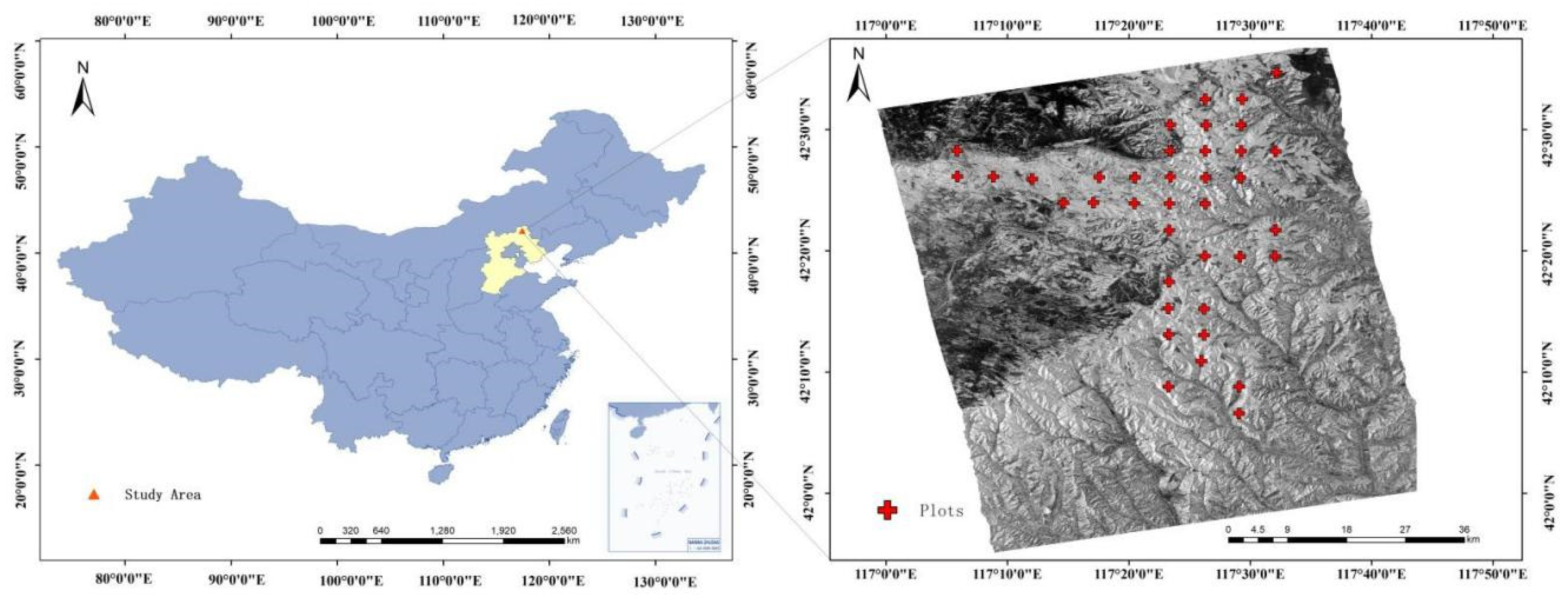
2. Study Area and Data
2.1. SAR Data
2.2. Field Data
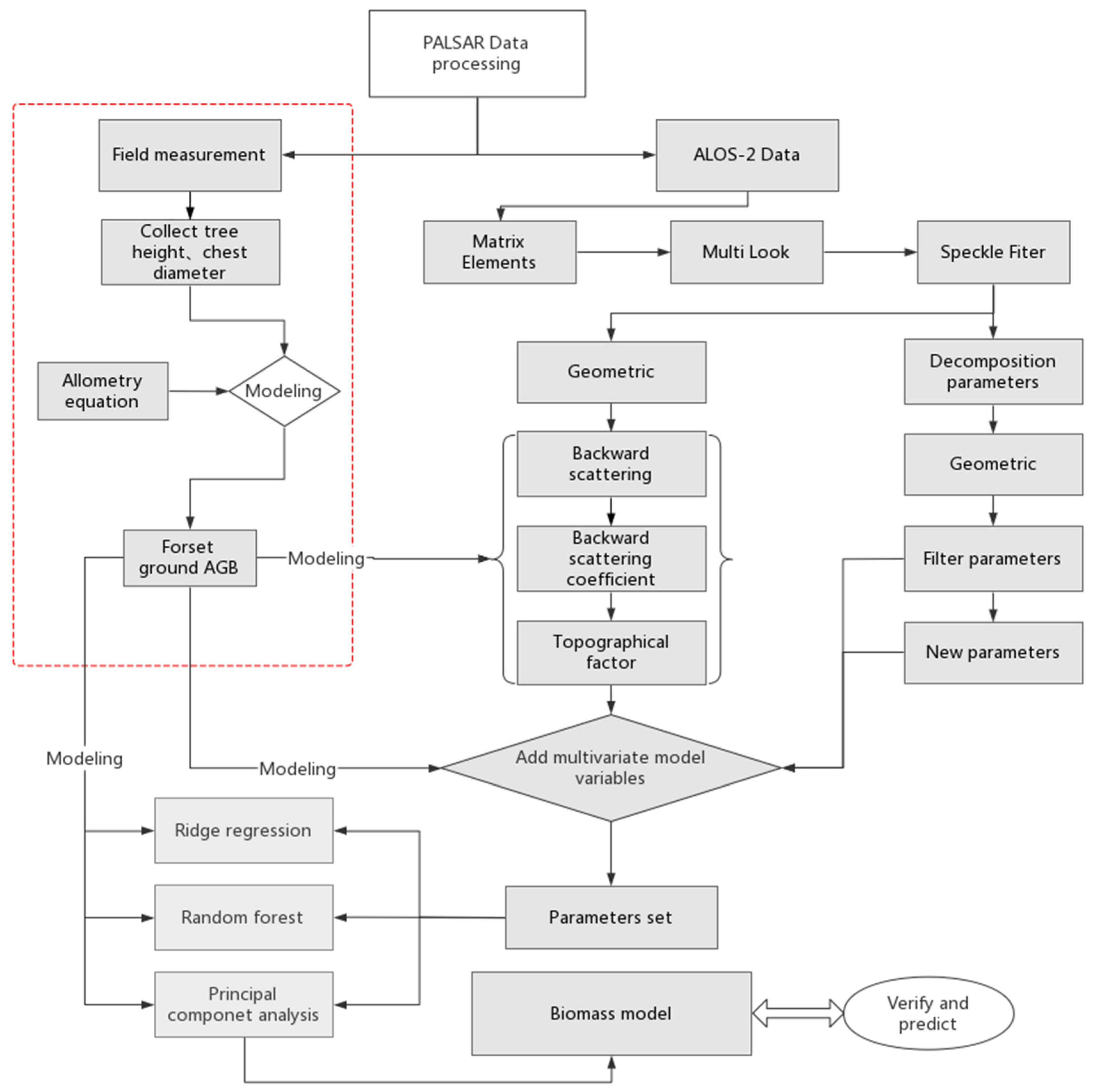
3. Methods
3.1. SAR Data Processing
3.2. Backscatter Coefficient and Its Combination
3.3. Terrain Factors
3.4. Constructing New Parameters
- Ground scattering—scattering parameter ratio;
- Even-scattering molecular parameters;
- Volume-scattering molecular parameters.
3.5. Multivariate Linear Model
3.6. Ridge Regression
3.7. Random Forest
3.8. Principal Component Analysis
3.9. Verification and Prediction
4. Results
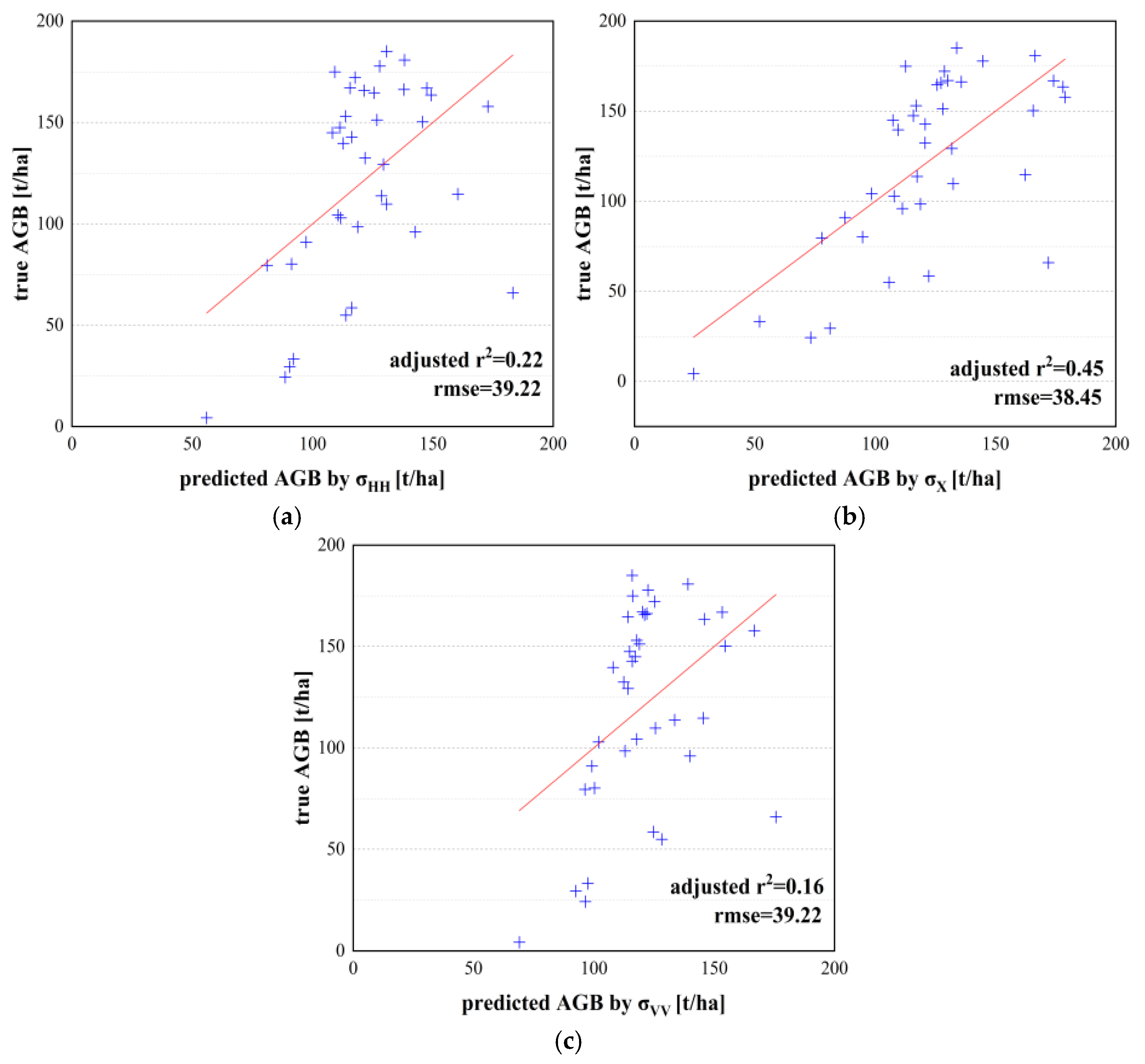
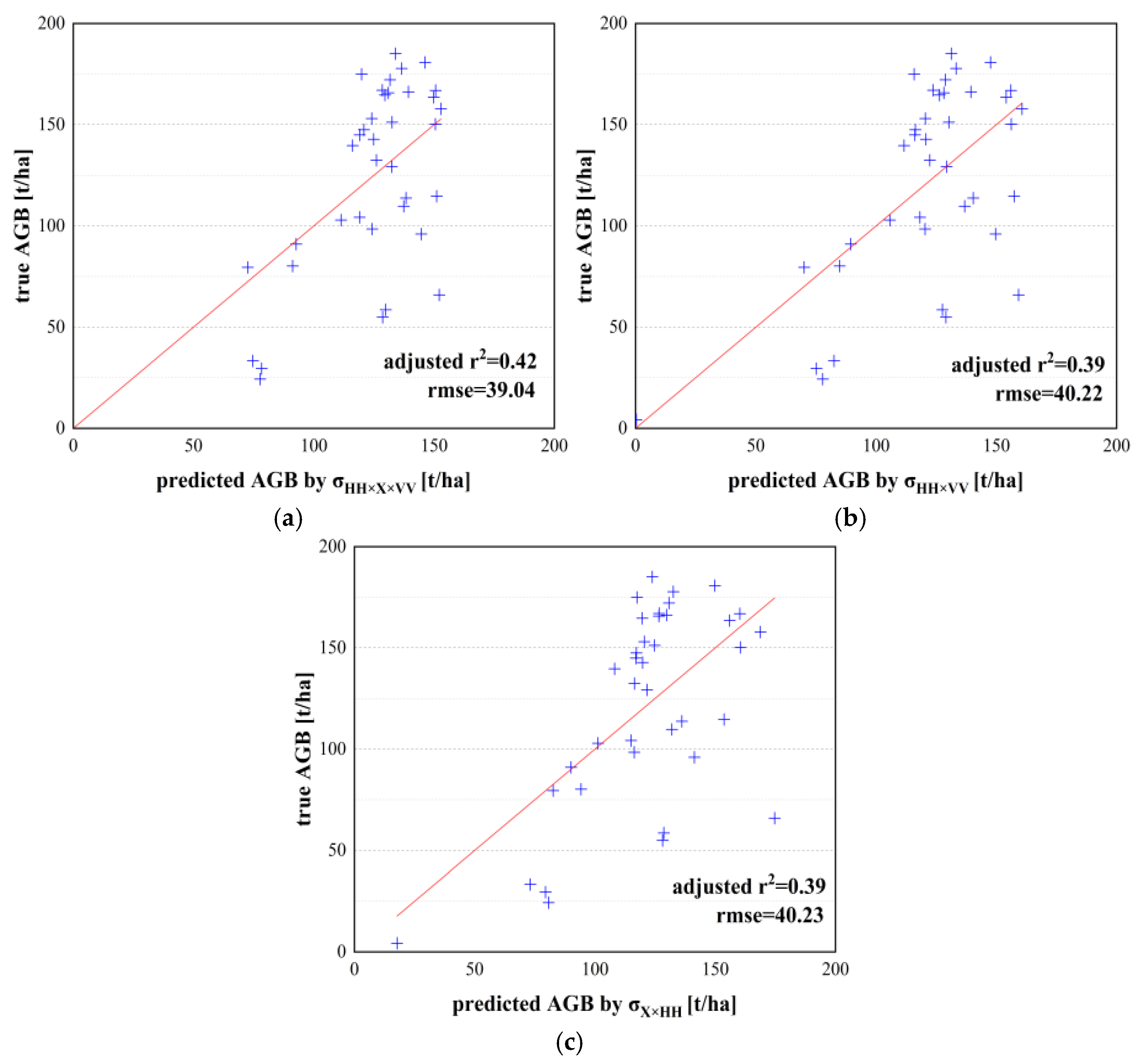
4.1. Backscatter Coefficient and Its Combination
4.2. Influence of Topographical Factors
4.3. New Parameters and AGB Estimation
4.4. Multivariate Linear Model
4.5. Ridge Regression Model
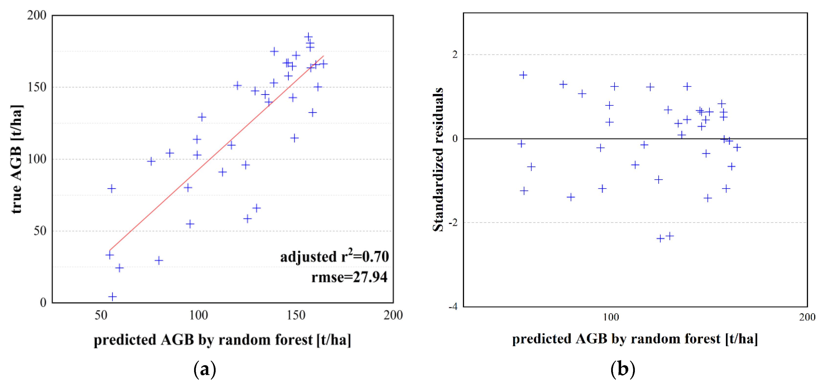
4.6. Random Forest
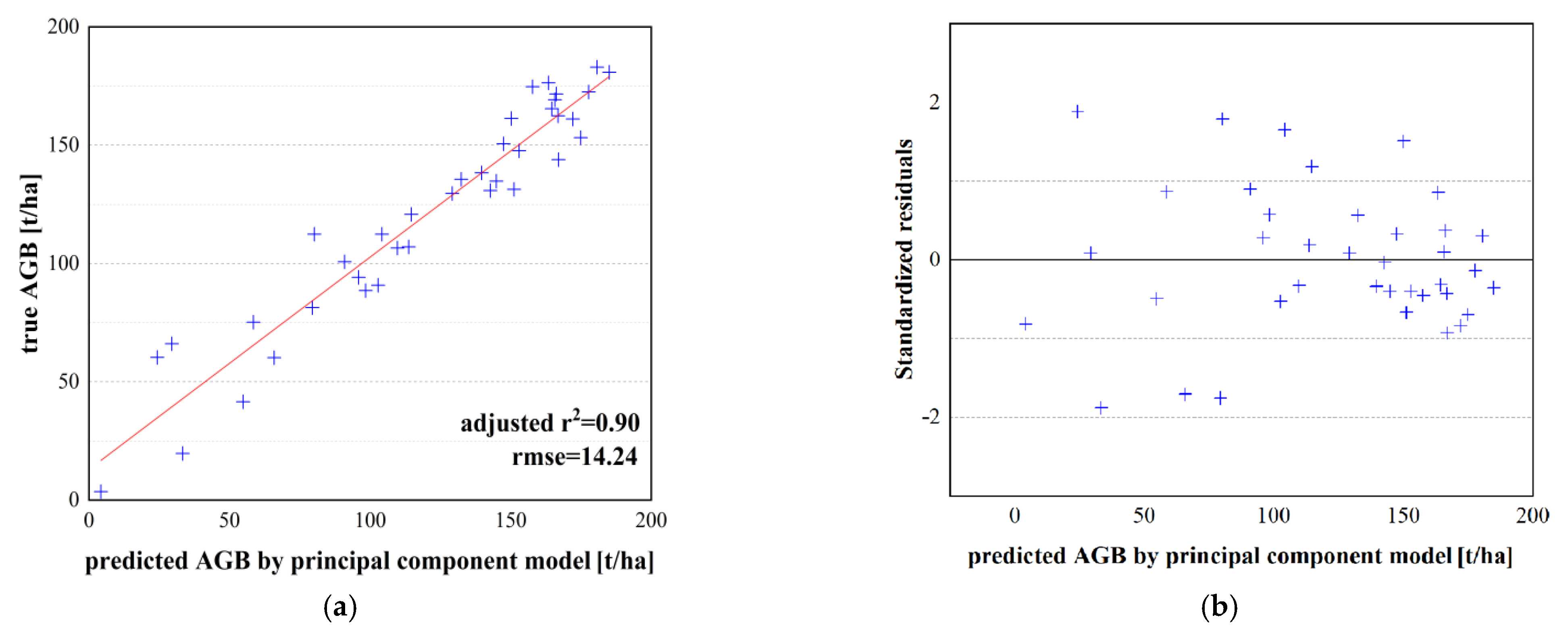
4.7. Principal Component Analysis
4.8. Model Selection and Prediction of the Study Area AGB
5. Discussion
6. Conclusions
- (1)
- The use of the backscatter coefficient to estimate AGB was more limited. The multivariate model provided better estimation capabilities than the univariate model. However, there was collinearity among the variables.
- (2)
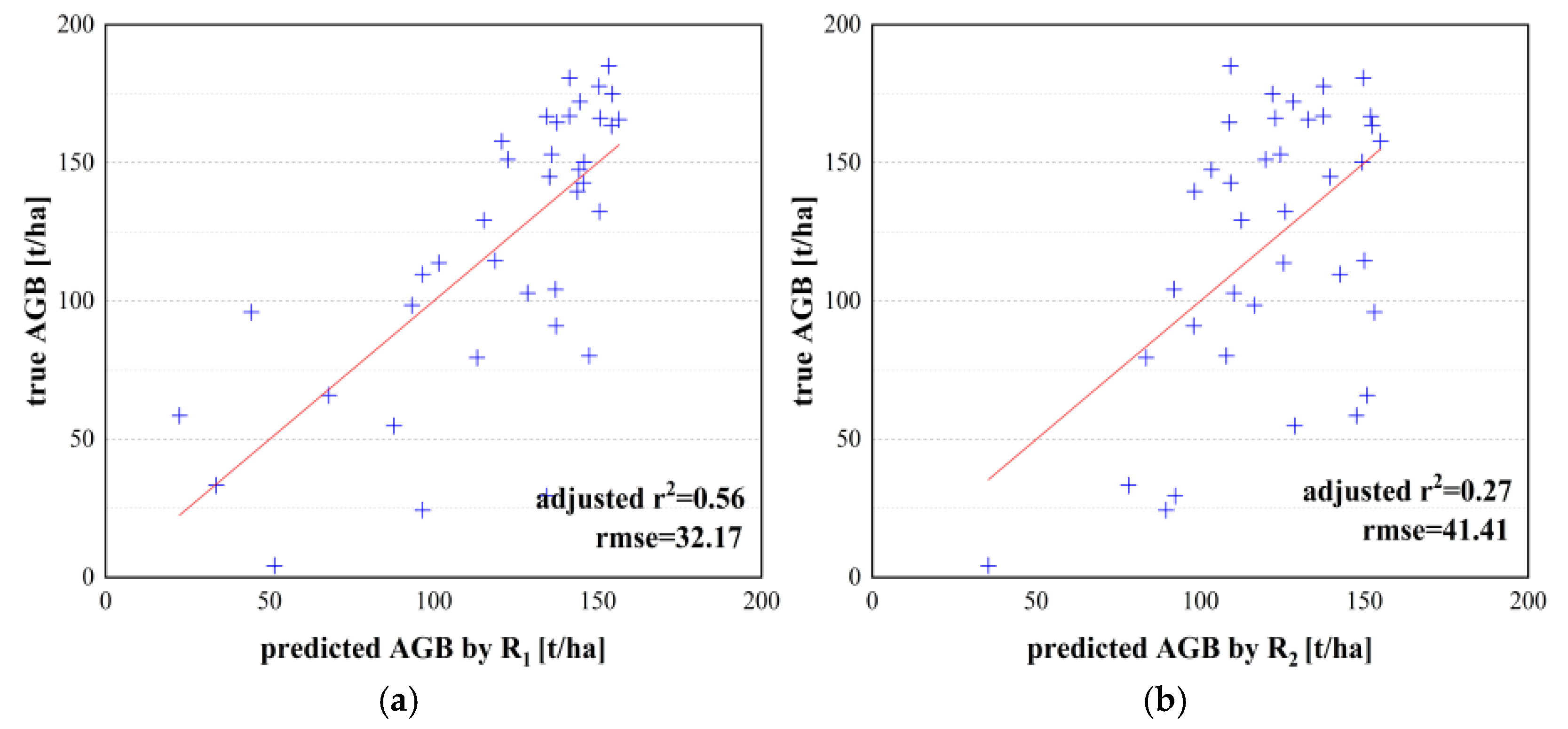
- The backscatter coefficient estimated that the AGB saturation point was low. The variable R1 improved the estimation of the saturation point.
- (3)
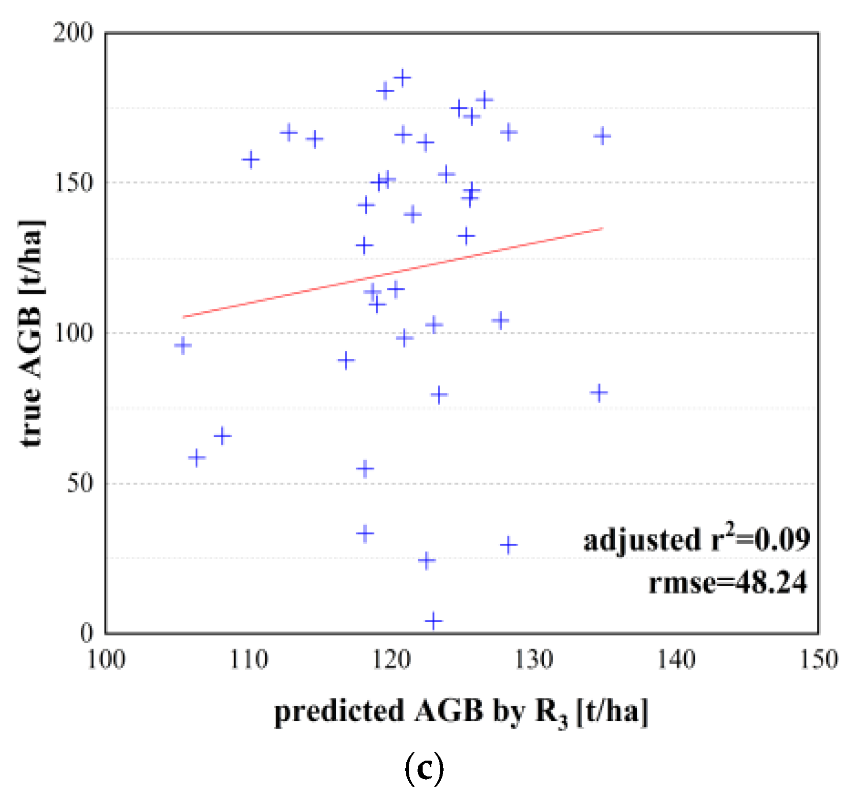
- The Earth-scattering ratio was more suitable for estimating AGB. This indicated that there was a degree of information complementarity between the variables. The combined backscatter coefficient was weak at estimating AGB.
- (4)
- The model established by combining the backscatter coefficients, terrain factors, and polarization decomposition parameters achieved high accuracy. The principal component analysis method was suitable for analyzing SAR data to estimate AGB. The final model effectively improved the saturation point of AGB.
Author Contributions
Funding
Acknowledgments
Conflicts of Interest
References
- Metcalf, C.J.E.; Graham, A.L.; Huijben, S.; Barclay, V.C.; Long, G.H.; Grenfell, B.T.; Read, A.F.; Bjørnstad, O.N. Partitioning Regulatory Mechanisms of Within-Host Malaria Dynamics Using the Effective Propagation Number. Science 2011, 333, 984–988. [Google Scholar] [CrossRef] [PubMed] [Green Version]
- Tanase, M.A.; Panciera, R.; Lowell, K. Airborne multi-temporal L-band polarimetric SAR data for biomass estimation in semi-arid forests. Remote Sens. Environ. 2014, 145, 93–104. [Google Scholar] [CrossRef]
- Blomberg, E.; Ferro-Famil, L.; Soja, M.J. Forest Biomass Retrieval From L-Band SAR Using Tomographic Ground Backscatter Removal. IEEE Geosci. Remote Sens. Lett. 2018, 15, 1030–1034. [Google Scholar] [CrossRef]
- Sinha, S.; Jeganathan, C.; Sharma, L.K. Nathawat, M.S.; Das, A.K.; Mohan, S. Developing synergy regression models with space-borne ALOS PALSAR and Landsat TM sensors for retrieving tropical forest biomass. J. Earth Syst. Sci. 2016, 125, 725–735. [Google Scholar] [CrossRef] [Green Version]
- Pulliainen, J.T.; Kurvonen, L.; Hallikainen, M.T. Multitemporal behavior of L- and C-band SAR observations of boreal forests. IEEE Trans. Geosci. Remote Sens. 1999, 37, 927–937. [Google Scholar] [CrossRef]
- Baghdadi, N.; le Maire, G.; Bailly, J.-S.; Ose, K.; Nouvellon, Y.; Zribi, M.; Lemos, C.; Hakamada, R. Evaluation of ALOS/PALSAR L-Band Data for the Estimation of Eucalyptus Plantations Aboveground Biomass in Brazil. IEEE J. Sel. Top. Appl. Earth Obs. Remote Sens. 2015, 8, 3802–3811. [Google Scholar] [CrossRef] [Green Version]
- Atwood, D.K.; Andersen, H.E.; Matthiss, B. Impact of Topographic Correction on Estimation of Aboveground Boreal Biomass Using Multi-temporal, L-Band Backscatter. IEEE J. Sel. Top. Appl. Earth Obs. Remote Sens. 2014, 7, 3262–3273. [Google Scholar] [CrossRef]
- Caicoya, A.T.; Pardini, M.; Hajnsek, I.; Papathanassiou, K. Forest Above-Ground Biomass Estimation from Vertical Reflectivity Profiles at L-Band. IEEE Geosci. Remote Sens. Lett. 2015, 12, 2379–2383. [Google Scholar] [CrossRef]
- Le Toan, T.; Beaudoin, A.; Riom, J.; Guyon, D. Relating forest biomass to SAR data. IEEE Trans. Geosci. Remote Sens. 1992, 30, 403–411. [Google Scholar] [CrossRef]
- Rignot, E.; Way, J.; Williams, C.; Viereck, L. Radar estimates of aboveground biomass in boreal forests of interior Alaska. IEEE Trans. Geosci. Remote Sens. 1994, 32, 1117–1124. [Google Scholar] [CrossRef] [Green Version]
- Ranson, K.; Sun, G. Mapping biomass of a northern forest using multifrequency SAR data. IEEE Trans. Geosci. Remote Sens. 1994, 32, 388–396. [Google Scholar] [CrossRef]
- Eini-Zinab, S.; Maghsoudi, Y.; Sayedain, S.A. Assessing the performance of indicators resulting from three-component Freeman–Durden polarimetric SAR interferometry decomposition at P-and L-band in estimating tropical forest aboveground biomass. Int. J. Remote Sens. 2019, 41, 433–454. [Google Scholar] [CrossRef]
- Golshani, P.; Maghsoudi, Y.; Sohrabi, H. Relating ALOS-2 PALSAR-2 Parameters to Biomass and Structure of Temperate Broadleaf Hyrcanian Forests. J. Indian Soc. Remote Sens. 2019, 47, 749–761. [Google Scholar] [CrossRef]
- Asari, N.; Suratman, M.N.; Jaafar, J. Modelling and mapping of above ground biomass (AGB) of oil palm plantations in Malaysia using remotely-sensed data. Int. J. Remote Sens. 2017, 38, 4741–4764. [Google Scholar] [CrossRef]
- Trisasongko, B.H.; Paull, D. A review of remote sensing applications in tropical forestry with a particular emphasis in the plantation sector. Geocarto Int. 2018, 35, 317–339. [Google Scholar] [CrossRef]
- Ranson, K.J.; Sun, G.; Weishampel, J.F.; Knox, R.G. Forest biomass from combined ecosystem and radar backscatter modeling. Remote Sens. Environ. 1997, 59, 118–133. [Google Scholar] [CrossRef]
- Kasischke, E.S.; Melack, J.M.; Dobson, M.C. The use of imaging radars for ecological applications—A review. Remote Sens. Environ. 1997, 59, 141–156. [Google Scholar] [CrossRef]
- Yu, Y.; Saatchi, S. Sensitivity of L-Band SAR Backscatter to Aboveground Biomass of Global Forests. Remote Sens. 2016, 8, 522. [Google Scholar] [CrossRef] [Green Version]
- Sarker, M.L.R.; Nichol, J.; Ahmad, B.; Busu, I.; Rahman, A.A. Potential of texture measurements of two-date dual polarization PALSAR data for the improvement of forest biomass estimation. ISPRS J. Photogramm. Remote Sens. 2012, 69, 146–166. [Google Scholar] [CrossRef]
- Lal, P.; Kumar, A.; Saikia, P.; Das, A.; Patnaik, C.; Kumar, G.; Pandey, A.C.; Srivastava, P.; Dwivedi, C.S.; Khan, M.L. Effect of vegetation structure on above ground biomass in tropical deciduous forests of Central India. Geocarto Int. 2021, 1, 1–17. [Google Scholar] [CrossRef]
- Baig, S.; Qazi, W.A.; Akhtar, A.M.; Waqar, M.M.; Ammar, A.; Gilani, H.; Mehmood, S.A. Above Ground Biomass Estimation of Dalbergia sissoo Forest Plantation from Dual-Polarized ALOS-2 PALSAR Data. Can. J. Remote Sens. 2017, 43, 297–308. [Google Scholar] [CrossRef]
- Freeman, A.; Durden, S.L. A three-component scattering model for polarimetric SAR data. IEEE Trans. Geosci. Remote Sens. 1998, 36, 963–973. [Google Scholar] [CrossRef] [Green Version]
- Zhang, Z.; Wang, Y.; Sun, G.; Ni, W.; Huang, W.; Zhang, L. Biomass Retrieval Based on Polarimetric Target Decomposition. In Proceedings of the IEEE International Geoscience and Remote Sensing Symposium, Vancouver, BC, Canada, 24–29 July 2011; pp. 1942–1945. [Google Scholar]
- Bharadwaj, P.S.; Kumar, S.; Kushwaha, S.; Bijker, W. Polarimetric scattering model for estimation of above ground biomass of multilayer vegetation using ALOS-PALSAR quad-pol data. Phys. Chem. Earth Parts A/B/C 2015, 83-84, 187–195. [Google Scholar] [CrossRef]
- Van Zyl, J.J.; Arii, M.; Kim, Y. Model-Based Decomposition of Polarimetric SAR Covariance Matrices Constrained for Nonnegative Eigenvalues. IEEE Trans. Geosci. Remote Sens. 2011, 49, 3452–3459. [Google Scholar] [CrossRef]
- Verma, A.; Haldar, D. SAR polarimetric analysis for major land covers including pre-monsoon crops. Geocarto Int. 2019, 36, 2224–2240. [Google Scholar] [CrossRef]
- Townsend, P.A. Estimating forest structure in wetlands using multitemporal SAR. Remote Sens. Environ. 2002, 79, 288–304. [Google Scholar] [CrossRef]
- Santos, J.R.; Freitas, C.C.; Araujo, L.S.; Dutra, L.V.; Mura, J.C.; Gama, F.F.; Soler, L.S.; Sant’Anna, S.J. Airborne P-band SAR applied to the aboveground biomass studies in the Brazilian tropical rainforest. Remote Sens. Environ. 2003, 87, 482–493. [Google Scholar] [CrossRef]
- Mougin, E.; Proisy, C.; Marty, G.; Fromard, F.; Puig, H.; Betoulle, J.; Rudant, J. Multifrequency and multipolarization radar backscattering from mangrove forests. IEEE Trans. Geosci. Remote Sens. 1999, 37, 94–102. [Google Scholar] [CrossRef]
- Hyde, P.; Nelson, R.; Kimes, D.; Levine, E. Exploring LiDAR–RaDAR synergy—predicting aboveground biomass in a southwestern ponderosa pine forest using LiDAR, SAR and InSAR. Remote Sens. Environ. 2007, 106, 28–38. [Google Scholar] [CrossRef]
- Wolpert, D.H.; Macready, W.G. An Efficient Method to Estimate Bagging’s Generalization Error. Mach. Learn. 1999, 35, 41–55. [Google Scholar] [CrossRef] [Green Version]
- Fu, W.; Guo, H.; Li, X. Relating Forest Biomass to the Polarization Phase Difference of the Double-Bounce Scattering Component. IEEE Geosci. Remote Sens. Lett. 2020, 18, 2048–2051. [Google Scholar] [CrossRef]
- Sharifi, A.; Amini, J. Forest biomass estimation using synthetic aperture radar polarimetric features. J. Appl. Remote Sens. 2015, 9, 097695. [Google Scholar] [CrossRef]
- Waqar, M.M.; Sukmawati, R.; Ji, Y.Q.; Sumantyo, J.T.S.; Segah, H.; Prasetyo, L.B. Retrieval of Tropical Peatland Forest Biomass from Polarimetric Features in Central Kalimantan, Indonesia. Prog. Electromagn. Res. C 2020, 98, 109–125. [Google Scholar] [CrossRef] [Green Version]
- Huang, X.; Ziniti, B.; Torbick, N.; Ducey, M.J. Assessment of Forest above Ground Biomass Estimation Using Multi-Temporal C-band Sentinel-1 and Polarimetric L-band PALSAR-2 Data. Remote Sens. 2018, 10, 1424. [Google Scholar] [CrossRef] [Green Version]
- Tanase, M.A.; Panciera, R.; Lowell, K.; Hacker, J.; Walker, J.P. Estimation of forest biomass from L-band polarimetric decomposition components. In Proceedings of the 2013 IEEE International Geoscience and Remote Sensing Symposium—IGARSS, Melbourne, VIC, Australia, 21–26 July 2013; pp. 949–952. [Google Scholar]
- Gleason, C.J.; Im, J. Forest biomass estimation from airborne LiDAR data using machine learning approaches. Remote Sens. Environ. 2012, 125, 80–91. [Google Scholar] [CrossRef]
- Mutanga, O.; Adam, E.; Cho, M.A. High density biomass estimation for wetland vegetation using WorldView-2 imagery and random forest regression algorithm. Int. J. Appl. Earth Obs. Geoinf. 2012, 18, 399–406. [Google Scholar] [CrossRef]
- Fassnacht, F.; Hartig, F.; Latifi, H.; Berger, C.; Hernández, J.; Corvalán, P.; Koch, B. Importance of sample size, data type and prediction method for remote sensing-based estimations of aboveground forest biomass. Remote Sens. Environ. 2014, 154, 102–114. [Google Scholar] [CrossRef]
- Sun, Z.; Liu, L.; Peng, S. Age-related modulation of the nitrogen resorption efficiency response to growth requirements and soil nitrogen availability in a temperate pine plantation. Ecosystems 2016, 19, 689–709. [Google Scholar] [CrossRef] [Green Version]
- Wang, C. Biomass allometric equations for 10 co-occurring tree species in Chinese temperate forests. For. Ecol. Manag. 2006, 222, 9–16. [Google Scholar] [CrossRef]
- Shimada, M.; Isoguchi, O.; Tadono, T. PALSAR radiometric and geometric calibration. IEEE Trans. Geosci. Remote Sens. 2009, 47, 3915–3932. [Google Scholar] [CrossRef]
- Lee, J.-S.; Grunes, M.; De Grandi, G. Polarimetric SAR speckle filtering and its implication for classification. IEEE Trans. Geosci. Remote Sens. 1999, 37, 2363–2373. [Google Scholar] [CrossRef]
- Gatelli, F.; Guamieri, A.M.; Parizzi, F. The wavenumber shift in SAR interferometry. IEEE Trans. Geosci. Remote Sens. 1994, 32, 855–865. [Google Scholar] [CrossRef] [Green Version]
- Varghese, A.O.; Suryavanshi, A.; Joshi, A.K. Analysis of different polarimetric target decomposition methods in forest density classification using C band SAR data. Int. J. Remote Sens. 2016, 37, 694–709. [Google Scholar] [CrossRef]
- Van Zyl, J.J. Application of Cloude’s Target Decomposition Theorem to Polarimetric Imaging Radar Data. In Proceedings of the SPIE Volume 1748, Radar Polarimetry, San Diego, CA, USA, 22 July 1992; SPIE: Bellingham, WA, USA, 1993. [Google Scholar] [CrossRef] [Green Version]
- Freeman, A. Fitting a Two-Component Scattering Model to Polarimetric SAR Data from Forests. IEEE Trans. Geosci. Remote Sens. 2007, 45, 2583–2592. [Google Scholar] [CrossRef]
- Yamaguchi, Y.; Moriyama, T.; Ishido, M.; Yamada, H. Four-component scattering model for polarimetric SAR image decomposition. IEEE Trans. Geosci. Remote Sens. 2005, 43, 1699–1706. [Google Scholar] [CrossRef]
- Yamaguchi, Y.; Yajima, Y.; Yamada, H. A Four-Component Decomposition of POLSAR Images Based on the Coherency Matrix. IEEE Geosci. Remote Sens. Lett. 2006, 3, 292–296. [Google Scholar] [CrossRef]
- Yamaguchi, Y.; Sato, A.; Boerner, W.-M.; Sato, R.; Yamada, H. Four-Component Scattering Power Decomposition with Rotation of Coherency Matrix. IEEE Trans. Geosci. Remote Sens. 2011, 49, 2251–2258. [Google Scholar] [CrossRef]
- Cui, Y.; Yamaguchi, Y.; Yang, J.; Park, S.-E.; Kobayashi, H.; Singh, G. Three-Component Power Decomposition for Polarimetric SAR Data Based on Adaptive Volume Scatter Modeling. Remote Sens. 2012, 4, 1559–1572. [Google Scholar] [CrossRef] [Green Version]
- Cloude, S.R.; Pottier, E. Concept of polarization entropy in optical scattering. Opt. Eng. 1995, 34, 1599–1610. [Google Scholar] [CrossRef]
- Touzi, R. Target Scattering Decomposition in Terms of Roll-Invariant Target Parameters. IEEE Trans. Geosci. Remote Sens. 2007, 45, 73–84. [Google Scholar] [CrossRef]
- Hyde, P.; Dubayah, R.; Walker, W.; Blair, J.B.; Hofton, M.; Hunsaker, C. Mapping forest structure for wildlife habitat analysis using multi-sensor (LiDAR, SAR/InSAR, ETM+, Quickbird) synergy. Remote Sens. Environ. 2006, 102, 63–73. [Google Scholar] [CrossRef]
- Zheng, D.; Rademacher, J.; Chen, J.; Crow, T.; Bresee, M.; Le Moine, J.; Ryu, S.-R. Estimating aboveground biomass using Landsat 7 ETM+ data across a managed landscape in northern Wisconsin, USA. Remote Sens. Environ. 2004, 93, 402–411. [Google Scholar] [CrossRef]
- Cloude, R.S.; Pottier, E. An entropy based classifification scheme for land applications of polarimetric SARs. IEEE Trans. Geosci. Remote Sens. 1997, 35, 68–78. [Google Scholar] [CrossRef]
- Anconitano, G.; Lavalle, M.; Arabini, E. Sensitivity to soil moisture by applying a model-based polarimetric decomposition to a time-series of airborne radar L-band data over an agricultural area. Microw. Remote Sens. Data Process. Appl. 2021, 11861, 1186105. [Google Scholar] [CrossRef]
- Simons-Legaard, E.; Legaard, K.; Weiskittel, A. Predicting aboveground biomass with LANDIS-II: A global and temporal analysis of parameter sensitivity. Ecol. Model. 2015, 313, 325–332. [Google Scholar] [CrossRef] [Green Version]
- Mette, T.; Papathanassiou, K.; Hajnsek, I. Biomass estimation from polarimetric SAR interferometry over heterogeneous forest terrain. In Proceedings of the IEEE International Geoscience and Remote Sensing Symposium, Anchorage, AK, USA, 20–24 September 2004. [Google Scholar]
- Sun, G.; Ranson, K.; Kharuk, V. Radiometric slope correction for forest biomass estimation from SAR data in the Western Sayani Mountains, Siberia. Remote Sens. Environ. 2002, 79, 279–287. [Google Scholar] [CrossRef]
- Ojoyi, M.; Mutanga, O.; Odindi, J.; Abdel-Rahman, E.M. Application of topo-edaphic factors and remotely sensed vegetation indices to enhance biomass estimation in a heterogeneous landscape in the Eastern Arc Mountains of Tanzania. Geocarto Int. 2015, 31, 1–21. [Google Scholar] [CrossRef]
- Aykut, T. Determination of groundwater potential zones using Geographical Information Systems (GIS) and Analytic Hierarchy Process (AHP) between Edirne-Kalkansogut (northwestern Turkey). Groundw. Sustain. Dev. 2021, 12, 100545. [Google Scholar] [CrossRef]
- Lee, J.-S. Grunes, M.; Pottier, E.; Ferro-Famil, L. Unsupervised terrain classification preserving polarimetric scattering characteristics. IEEE Trans. Geosci. Remote Sens. 2004, 42, 722–731. [Google Scholar] [CrossRef]
- Chowdhury, T.A.; Thiel, C.; Schmullius, C.; Stelmaszczuk-Górska, M. Polarimetric Parameters for Growing Stock Volume Estimation Using ALOS PALSAR L-Band Data over Siberian Forests. Remote Sens. 2013, 5, 5725–5756. [Google Scholar] [CrossRef] [Green Version]
- Martínez, A.M.; Kak, A.C. PCA versus LDA. IEEE Trans. Pattern Anal. Mach. Intell. 2001, 23, 228–233. [Google Scholar] [CrossRef] [Green Version]
- Castaño-Díaz, M.; Barrio-Anta, M.; Afif-Khouri, E.; Cámara-Obregón, A. Willow Short Rotation Coppice Trial in a Former Mining Area in Northern Spain: Effects of Clone, Fertilization and Planting Density on Yield after Five Years. Forests 2018, 9, 154. [Google Scholar] [CrossRef] [Green Version]
- Wong, T.T. Performance evaluation of classification algorithms by k-fold and leave-one-out cross validation. Pattern Recognit. 2015, 48, 2839–2846. [Google Scholar] [CrossRef]
- Quint, T.C.; Dech, J. Allometric models for predicting the aboveground biomass of Canada yew (Taxus canadensis Marsh.) from visual and digital cover estimates. Can. J. For. Res. 2010, 40, 2003–2014. [Google Scholar] [CrossRef]
- Solberg, S.; Astrup, R.; Gobakken, T.; Næsset, E.; Weydahl, D.J. Estimating spruce and pine biomass with interferometric X-band SAR. Remote Sens. Environ. 2010, 114, 2353–2360. [Google Scholar] [CrossRef]
- Wold, S.; Esbensen, K.; Geladi, P. Principal component analysis. Chemom. Intell. Lab. Syst. 1987, 2, 37–52. [Google Scholar] [CrossRef]
- Neumann, M.; Saatchi, S.S.; Ulander, L.M.H.; Fransson, J.E.S. Assessing Performance of L- and P-Band Polarimetric Interferometric SAR Data in Estimating Boreal Forest Above-Ground Biomass. IEEE Trans. Geosci. Remote Sens. 2012, 50, 714–726. [Google Scholar] [CrossRef]
- Kobayashi, S.; Omura, Y.; Sanga-Ngoie, K.; Widyorini, R.; Kawai, S.; Supriadi, B.; Yamaguchi, Y. Characteristics of Decomposition Powers of L-Band Multi-Polarimetric SAR in Assessing Tree Growth of Industrial Plantation Forests in the Tropics. Remote Sens. 2012, 4, 3058–3077. [Google Scholar] [CrossRef] [Green Version]


| Number | AGB (t/ha) | Number | AGB (t/ha) | Number | AGB (t/ha) | Number | AGB (t/ha) |
|---|---|---|---|---|---|---|---|
| 01 | 129.252 | 11 | 80.171 | 21 | 172.128 | 31 | 54.836 |
| 02 | 142.776 | 12 | 174.936 | 22 | 166.592 | 32 | 167.011 |
| 03 | 139.653 | 13 | 147.477 | 23 | 98.417 | 33 | 165.710 |
| 04 | 58.508 | 14 | 153.008 | 24 | 104.223 | 34 | 144.930 |
| 05 | 166.223 | 15 | 185.083 | 25 | 151.198 | 35 | 109.724 |
| 06 | 4.248 | 16 | 177.771 | 26 | 164.641 | 36 | 95.931 |
| 07 | 113.727 | 17 | 163.469 | 27 | 180.735 | 37 | 24.281 |
| 08 | 79.486 | 18 | 157.807 | 28 | 102.843 | 38 | 33.292 |
| 09 | 29.471 | 19 | 65.888 | 29 | 150.238 | ||
| 10 | 132.427 | 20 | 90.952 | 30 | 114.632 |
| Method | Parameter | |
|---|---|---|
| Yamaguchi three-component decomposition | Odd scattering component of Yamaguchi 3 decomposition (YamaguchiOdd) Even scattering component of Yamaguchi 3 decomposition (YamaguchiDbl) Scattering component of Yamaguchi 3 decomposition volume (YamaguchiVol) | |
| H/A/alpha eigenvalue set decomposition | Eigenvalue | anisotropy, ansiotropy_lueneburg, anisotropy 12 asymetry, derd, derd_norm, entropysh, entropy 1 entropy 2, entropy 3, entropy 4, entropy 5, I1, I2, I3, p1, p2, p3, prdestal, polarisation_fraction rvi, serd, serd_norm |
| H/A/alpha eigenvector set decomposition | Eigenvector | alpha, alpha1, alpha 2, alpha 3 beta, beta 1, beta 2, beta 3 delta, delta 1, delta 2, delta 3 gamma, gamma1, gamma 2, gamma 3 |
| Correlation Coefficient | Backscatter Coefficients | ||
|---|---|---|---|
| Person coefficient | 0.497 ** | 0.680 ** | 0.425 ** |
| Parameter | Pearson Coefficient | Parameter | Pearson Coefficient | Parameter | Pearson Coefficient |
|---|---|---|---|---|---|
| −0.154 | −0.060 | 0.102 | |||
| −0.200 | −0.093 | −0.217 | |||
| −0.093 | 0.144 | 0.243 | |||
| 0.043 | −0.060 | −0.263 | |||
| −0.154 | 0.143 | −0.232 | |||
| −0.148 | −0.148 | −0.637 ** | |||
| −0.200 | 0.285 | −0.631 ** | |||
| −0.066 | 0.117 | 0.666 ** | |||
| 0.143 | 0.244 |
| Parameters | Topographical Factors | ||
|---|---|---|---|
| Slope | Elevation | Aspect | |
| Pearson coefficient | 0.417 ** | 0.162 | 0.223 |
| Correlation Coefficient | New Parameter | ||
|---|---|---|---|
| R1 | R2 | R3 | |
| Pearson coefficient | −0.756 ** | −0.322 | 0.190 |
| Correlation Coefficient | Decomposition Parameter | ||||
|---|---|---|---|---|---|
| Entropysh | Entropy 1 | Entropy 2 | Entropy 3 | Gamma 3 | |
| Pearson coefficient | 0.672 ** | 0.596 ** | 0.617 ** | 0.696 ** | 0.439 ** |
| I2 | I3 | YamaguchiVol | YamaguchiDbl | ||
| Pearson coefficient | 0.667 ** | 0.635 ** | 0.623 ** | 0.697 ** | |
| Variable | Dimension | Sig | Vif |
|---|---|---|---|
| 1 | 0.607 | 84.422 | |
| 2 | 0.251 | 689.347 | |
| 3 | 0.925 | 150.481 | |
| 4 | 0.150 | 346.537 | |
| 5 | 0.448 | 2571.564 | |
| 6 | 0.126 | 444.793 | |
| entropysh | 7 | 0.656 | 1798.225 |
| entropy 1 | 8 | 0.648 | 218.010 |
| entropy 22 | 9 | 0.070 | 335.184 |
| entropy 33 | 10 | 0.015 | 153.786 |
| gamma 3 | 11 | 0.648 | 1.585 |
| I2 | 12 | 0.535 | 295.838 |
| I3 | 13 | 0.935 | 792.565 |
| R1 | 14 | 0.999 | 17.052 |
| YamaguchiVol | 15 | 0.898 | 1125.782 |
| YamaguchiDbl | 16 | 0.531 | 59.219 |
| Kaiser–Meyer–Olkin Sampling Suitability | 0.746 | |
|---|---|---|
| Bartlett’s Test | Approximated chi-square | 1753.496 |
| Degree of freedom | 136 | |
| Significance | 0.000 | |
| Variable | Principal Component Coefficient | |
|---|---|---|
| Factor 1 | Factor 2 | |
| 0.904 | −0.310 | |
| 0.962 | −0.305 | |
| 0.900 | −0.331 | |
| −0.915 | 0.237 | |
| −0.933 | 0.209 | |
| 0.877 | −0.185 | |
| entropysh | 0.982 | 0.053 |
| entropy 1 | 0.972 | −0.056 |
| entropy 22 | 0.966 | 0.082 |
| entropy 33 | 0.953 | −0.002 |
| gamma 3 | 0.227 | 0.458 |
| I2 | 0.924 | 0.240 |
| I3 | 0.905 | 0.239 |
| R1 | −0.349 | −0.795 |
| YamaguchiVol | 0.900 | 0.229 |
| YamaguchiDbl | 0.847 | 0.287 |
| Component | Eigenvalue | Cumulative | ||||
|---|---|---|---|---|---|---|
| Aggregate | Variance (%) | Total (%) | Aggregate | Variance (%) | Total (%) | |
| Factor 1 | 12.161 | 71.538 | 71.538 | 12.161 | 71.538 | 71.538 |
| Factor 2 | 1.541 | 9.068 | 80.606 | 1.541 | 9.068 | 80.606 |
| Parameter | Unstandardized Coefficient | Student’s Test Value | Sig | Vif |
|---|---|---|---|---|
| Constant | 112.635 | 39.083 | 0.000 | |
| Factor 1 | 34.427 | 10.982 | 0.000 | 1.000 |
| Factor 2 | −29.648 | −9.458 | 0.000 | 1.000 |
| Type | Model | Evaluation Index | |||||
|---|---|---|---|---|---|---|---|
| Adjusted r2 | RMSE (t/ha) | ME (t/ha) | MAE (t/ha) | MARE (%) | MRE (%) | ||
| Unary model | and AGB model | 0.45 | 38.45 | 1.17 | 37.22 | 45.51 | 17.71 |
| and AGB model | 0.42 | 39.04 | 3.15 | 32.94 | 44.30 | 21.25 | |
| R1 and AGB model | 0.56 | 32.17 | 1.82 | 25.69 | 39.17 | 8.77 | |
| Multivariate model | 0.87 | 17.42 | −0.12 | 14.82 | 27.35 | 15.25 | |
| Ridge regression model | 0.63 | 30.25 | −0.04 | 23.18 | 36.22 | 17.32 | |
| Principal component model | 0.90 | 14.24 | −0.023 | 10.96 | 18.92 | 5.03 | |
| Random forest model | 0.70 | 27.94 | −1.99 | 23.04 | 23.21 | 17.44 | |
Publisher’s Note: MDPI stays neutral with regard to jurisdictional claims in published maps and institutional affiliations. |
© 2022 by the authors. Licensee MDPI, Basel, Switzerland. This article is an open access article distributed under the terms and conditions of the Creative Commons Attribution (CC BY) license (https://creativecommons.org/licenses/by/4.0/).
Share and Cite
Liu, Z.; Michel, O.O.; Wu, G.; Mao, Y.; Hu, Y.; Fan, W. The Potential of Fully Polarized ALOS-2 Data for Estimating Forest Above-Ground Biomass. Remote Sens. 2022, 14, 669. https://doi.org/10.3390/rs14030669
Liu Z, Michel OO, Wu G, Mao Y, Hu Y, Fan W. The Potential of Fully Polarized ALOS-2 Data for Estimating Forest Above-Ground Biomass. Remote Sensing. 2022; 14(3):669. https://doi.org/10.3390/rs14030669
Chicago/Turabian StyleLiu, Zhihui, Opelele Omeno Michel, Guoming Wu, Yu Mao, Yifan Hu, and Wenyi Fan. 2022. "The Potential of Fully Polarized ALOS-2 Data for Estimating Forest Above-Ground Biomass" Remote Sensing 14, no. 3: 669. https://doi.org/10.3390/rs14030669
APA StyleLiu, Z., Michel, O. O., Wu, G., Mao, Y., Hu, Y., & Fan, W. (2022). The Potential of Fully Polarized ALOS-2 Data for Estimating Forest Above-Ground Biomass. Remote Sensing, 14(3), 669. https://doi.org/10.3390/rs14030669