Abstract
Synthetic aperture radar (SAR) frequently suffers from radio frequency interference (RFI) due to the simultaneous presence of numerous wireless communication signals. Recently, the narrowband RFI is found to possess the low-rank property benefiting from stable frequency occupancy, hence the reconsideration of RFI suppression as a joint sparse and low-rank optimization problem. The existing methods either use the non-sparse useful signal itself as the sparse regularizer, or employ the nuclear norm to approximate the rank function, which punishes all singular values with the same penalty via singular value thresholding (SVT), resulting in the improper punishment problem. Hence, both are consequentially subject to performance limitation. In this paper, a novel dictionary-based nonconvex low-rank minimization (DNLRM) optimization framework is proposed for RFI suppression, which concurrently considers the improvements for both the sparse regularizer and the low-rank regularizer. For the former, an over-completed dictionary is constructed, for which the sparse coefficient acts as the sparse regularizer. For the latter, the rank function is more accurately approximated by innovatively introducing the nonconvex function, for which the supergradient is synchronously used to generate the weighted penalty, thus solving the improper punishment problem. The derivation of the closed-form solution and the convergence analysis are described in detail. Additionally, the adaptive selection scheme for the model parameter is uniquely proposed for further ensuring the practicality of the DNLRM framework. The superiority of the proposed method is demonstrated via not only the RFI-free real SAR data combined with the measured RFI, but the RFI-contaminated real SAR data.
1. Introduction
Synthetic aperture radar (SAR) is an active remote sensing instrument that has been widely used for Earth observation with the special capability of working all-time and all-weather [1,2]. Due to the increasingly complex electromagnetic environment, SAR frequently suffers from radio frequency interference (RFI). RFI can cause degradation to image quality, which appears as misty streaks in the imaging result. The RFI-contaminated SAR images can even affect subsequent operations, such as polarimetry, interferometry, and target detection [3,4,5,6], thus highlighting the importance of RFI suppression.
Recently, for narrowband RFI suppression, the previous literature has put forward plenty of effective methods, which can be divided into three categories, namely nonparametric methods [7,8,9,10,11,12,13], parametric methods [14,15,16], and semiparametric methods [17,18,19,20,21,22,23]. The common nonparametric methods include the notched filtering (NF) method [7,8], the eigen-subspace projection (ESP) method [9,10], and the LMS filtering method [11,12,13]. The NF method is convenient for implementation, but in a severe RFI environment, the accompanying discontinuous spectrum will introduce artifacts into the SAR images. The singular value decomposition (SVD)-based ESP method suppresses RFI by constructing and separating the RFI subspace, but the RFI remnants or loss of useful signals occurs if the singular values belonging to the RFIs are misclassified. The LMS filtering method can cause the large distortion of signal phases then results in asymmetrical sidelobes [13]. Additionally, it may face greater challenges when the spectrum of different interferences is interconnected, which is often the case in complex electromagnetic environments [3].
As for the parametric methods, modeling the narrowband RFI as a sum of several sinusoids, many researches concentrate on estimating both the amplitudes and frequencies of the sinusoids to represent RFI more precisely. To date, the representative researches include the complex empirical mode decomposition method [14], the RELAX method [15], and the iterative adaptive method [16]. From the view of information capture, the above parametric methods can achieve a better RFI suppression performance for having gained more information about RFI than the nonparametric methods. However, this is based on the degree by which the parametric model matches the actual RFI-contaminated SAR signal, since the non-sinusoidal useful signal results in the occurrence of side effects on the estimation and the acquirement of the sinusoid-like RFI.
The newly proposed semiparametric methods especially consider the low-rank property of a two-dimensional RFI matrix, which is generated by stacking multiple pulses along the azimuth [17,18,19,20,21,22,23]. The low-rank property benefits from the fact that RFI usually occupies constant frequencies within the SAR working band for a period of time, which ensures its high degree of correlation in azimuth. Some of the existing literature models RFI as the low-rank matrix, meanwhile, the useful SAR signal is directly regularized as the sparse part, which also exists for the purpose of protection [22,23]. The above modeling framework is the classic form of robust principal component analysis (RPCA), which is widely used in background acquisition [24], image denoising [25], and moving target detection [26]. Recently, the consideration of RPCA pioneers the usage of the low-rank characteristics of RFI for signal separation. At the same time, there are also corresponding deficiencies, which are mainly reflected in two aspects. Firstly, it is inappropriate to directly use the useful signal itself as a sparse regularizer, which is, however, the case in most of the literature [18,19,20]. For a common pulse compression SAR system, such as the linear frequency modulation (LFM) SAR, the LFM signal is considered in the transmitter. If the LFM-based useful signal, which is noise-like and thus non-sparse, is directly used as the sparse regularization without pulse compression, the performance of the optimization model is inevitably limited. Secondly, the low-rank models proposed in most of the literature [17,18,19,21] approximate the rank function of the two-dimension RFI matrix with the sum of all the singular values, namely the nuclear norm. The corresponding low-rank minimization problem can be solved by the singular value thresholding (SVT) algorithm, whereas for the nuclear norm, the SVT algorithm punishes all the singular values with the same penalty [27,28]. This is evidently not in conformity with the reality that larger singular values, which stand for RFIs, should be less punished. Generally, there are two disadvantages once the same penalty has been used. If the penalty is large, to a certain extent, the over-punishment of RFI occurs and the interference pattern is left in the imaging result due to the residual RFIs. If the penalty is small enough, the under-punishment of useful signals occurs and part of the useful signal is included into RFIs, resulting in a significant reduction in the final imaging quality.
For the former sparsity-related problem, one possible solution is to construct an over-completed dictionary from the discrete time-shifted versions of the transmitted signal [17,21,29]. Therefore, with the corresponding dictionary, the sparse coefficient is used for the sparse regularization, while the improper punishment is still ignored in the researches mentioned above. In order to approximate the rank function more accurately and solve the improper punishment problem concerning the latter low-rank-related issue, the reweighted nuclear norm (RNN) method [20] firstly considers a scheme to calculate the weighted penalties based on the reciprocal of the singular values. Nevertheless, the theoretical basis for the rank approximation is not explicitly presented, and the influence of the weighting function on the updating of the low-rank matrix is not clearly analyzed. Furthermore, the non-sparse useful signal is directly used as the sparse regularization and, thus, the restricted performance. Moreover, the preceding studies barely investigated the combination of simultaneously using the over-completed dictionary and approximating the rank function in a more accurate way, let alone analyzing the behavior of the weighting function in the punishment operation.
Considering the above problems, to mitigate the limitation of RFI suppression performance caused by inaccurate modeling, the dictionary-based nonconvex low-rank minimization (DNLRM) framework is innovatively proposed in this paper to more accurately model the entire RFI suppression problem, with the reason being twofold. Firstly, nonconvex functions are introduced to approximate the rank function more accurately. Note that this is the first attempt to suppress RFIs using nonconvex functions. The improper punishment problem in terms of singular values can be overcome by treating larger ones with smaller penalties. Noteworthily, the supergradient of the nonconvex function is directly related to the calculation of the weighted penalty [30,31,32,33]. Secondly, an over-completed dictionary constructed by the discrete time-shifted versions of the transmitted signal is considered. Therefore, the corresponding sparse coefficient, rather than the useful signal itself, is used as the sparse regularizer for better modeling and protection. The constructed dictionary is inspired by [17,21,29], but is also combined with nonconvex functions for the first time, then further applied to our new framework. Benefitting from the discrimination for different singular values, the obtained low-rank matrix can better represent RFIs, and the useful signal protected by the sparser regularization has better fidelity with less residual RFIs. In addition, after an in-depth analysis of the behavior of the weighting function in the punishment operation, the adaptive selection scheme for the model parameter in DNLRM (ADNLRM) is uniquely proposed, based on a modified boxplot. Adaptively searching the optimal parameter for weighting functions without human intervention, ADNLRM can further improve the practicality of the proposed framework.
In conclusion, the main contributions of this paper are embodied in the following three aspects:
- (1)
- The DNLRM framework is innovatively proposed to solve the inaccurate modeling problems and unify the preceding similar methods. The alternating direction method of multiplier (ADMM)-based detailed derivation for the closed-form solution is provided, along with the convergence analysis.
- (2)
- Different nonconvex functions and the corresponding supergradients are originally introduced into RFI suppression to overcome the improper punishment problem. Additionally, ADNLRM is uniquely proposed for adaptively selecting the optimal parameter, which improves the applicability for varying RFI suppression missions.
- (3)
- The artificial combination of the RFI-free real SAR data with the measured RFI are considered alongside the RFI-contaminated real SAR data, to further verify the practicability of the proposed methods in a realistic environment.
The remainder of this paper is organized as follows. Section 2 reviews the RFI-contaminated SAR signal model and basic optimization frameworks. The proposed DNLRM framework with the corresponding formula derivation, and the adaptive selection scheme (ADNLRM) are described in Section 3. Section 4 presents the optimization framework analysis. Section 5 reports the experiment results and discussions. Finally, Section 6 summarizes the conclusions and presents future prospects in the discipline.
2. Materials
2.1. Signal Model
In the stop-and-go model, SAR mounted on the moving platform sends and receives signals at each azimuth position. Benefiting from its high two-dimensional matching gain, SAR can obtain high-resolution images of the target scene and clearly display the details of the objects of interest. On the other hand, as an active microwave system, SAR often shares the working frequency bandwidth with other forms of electromagnetic signals. The presence of RFI seriously affects the quality of SAR imaging, which is certainly detrimental to the implementation of SAR image interpretation.
In a crowded electromagnetic environment, SAR may always receive mixed data consisting of the useful signal , RFI , and noise , which can be formulated as:
where represents the received signal, and and are, respectively, the fast time and the slow time. The useful signal and RFI overlap in the time domain, thus they are difficult to separate directly. Therefore, it is necessary to find a suitable domain where their energy is separated from each other to effectively perform RFI separation and suppression. The signal form of is relevant to the transmitted signal. For a linear frequency modulation (LFM) SAR system, is the corresponding LFM signal. Meanwhile, narrowband RFI can usually be modeled as the sum of sinusoid-like components as:
where is the complex envelope, is the carrier frequency, and is the initial phase of the rth sinusoid RFI component. This concise model proves to be suitable to describe narrowband RFI.
If the received signals are stacked along the azimuth, the corresponding two-dimensional SAR data matrix can be obtained. The received signal , with and respectively denoting the samples along range and the number of pulses along azimuth, can thus be formulated as:
where , , and are, respectively, the useful signals, RFI, and additive white Gaussian noises in the matrix form. Considering the signal from the perspective of the two-dimensional matrix, we can further extract the signal property, which cannot be revealed by the traditional one-dimensional analysis. Therefore, under the premise of accurately exploring the signal property and appropriately establishing the optimization model, the RFI suppression mission can be reconsidered as a matrix separation problem.
2.2. Optimization Frameworks
Once the two-dimensional SAR data matrix is transformed into the range–frequency and azimuth–time domains, thin and bright stripes appear along the azimuth time, as shown in Figure 1a. Such a high correlation in the azimuth time is the fundamental source for RFI being low-rank. The available low-rank property of RFI, benefiting from its stable frequency occupancy, indicates the singular values’ precipitously dropping down, as shown in Figure 1b. The amplitudes of the singular values were normalized based on the Frobenius norm of the RFI matrix. Additionally, the normalized RFI spectrum of a certain azimuth pulse marked in the red ellipse is shown in Figure 1c, which reveals its complexity and diversity. The extraction of the low-rank component can be obtained by a minimization of the rank function. Additionally, the sparsity of the useful signal should be regularized by an norm for protection purposes [22,23]. To sum up, the RFI separation is accomplished via the following optimization:
where rank means the rank function, acts as a weighting factor between the low-rank RFI and the useful signal, denotes the norm, denotes the Frobenius norm, and is a fairly small positive number. As mentioned in [17,21], the useful signal is noise-like and non-sparse, thus not suitable for sparse regularization directly. One alternative scheme considers the sparsity under the over-completed dictionary, , constructed by the time-shifted version of the transmitted signal [29,34], where represents the number of atoms in the dictionary. Therefore, the corresponding optimization is modeled as:
where is the corresponding sparse coefficient of the useful signal under dictionary .

Figure 1.
Description of RFI features: (a) measured RFI in the range-frequency and azimuth-time domains, (b) the corresponding singular value distribution, and (c) RFI spectrum corresponding to the certain pulses marked in the red ellipse of (a).
For the NP-hard peculiarity of the above optimization, the rank function and norm are usually relaxed to the nuclear norm and the norm respectively, thus resulting in the following optimization:
Such an optimization can be solved by the ADMM method [35,36], which successively decomposes and deals with the subproblem and the subproblem. For the subproblem in the form of the nuclear norm, the SVT algorithm is used to generate a closed-form solution. However, different singular values are treated with the same penalty level, which can result in an incomplete RFI separation. As large singular values belong to the RFIs, they need less punishment. Therefore, a dictionary-based nonconvex low-rank minimization optimization framework is proposed and described in detail in Section 3.
3. Methods
In this section, the nonconvex regularizer and the corresponding supergradient are firstly analyzed in a comparative manner. Subsequently, the proposed DNLRM framework is described in detail, including the establishment of the framework and the ADMM-based derivation of the closed-form solution. Furthermore, after carefully considering the relation between the weighting function and singular values, the adaptive selection scheme ADNLRM for the model parameter is originally provided to further ensure the practicability of the proposed framework.
3.1. Nonconvex Regularizer
Inspired by [30], which suggests that the nonconvex sparse optimization usually outperforms convex models and summarizes several common nonconvex functions, the nonconvex regularizer is innovatively introduced into the RFI suppression mission under our specific consideration. Figure 2a shows the nonconvex functions for approximating the rank function with the corresponding supergradients illustrated in Figure 2c. The definitions of the considered nonconvex functions are formulated as:
and the corresponding supergradients are:
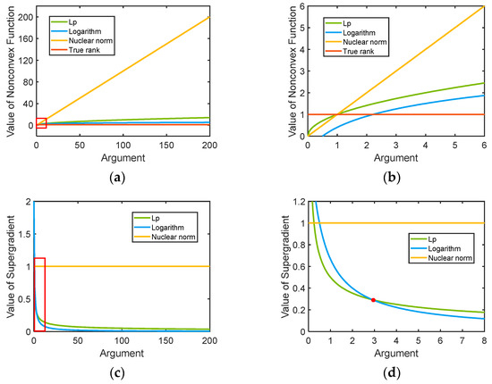
Figure 2.
Curve comparison: (a) illustrates the different functions for approximating the rank function, and the dense region in the red square is enlarged into (b). (c) Shows the corresponding supergradients where , , and the curves in the red rectangle are enlarged into (d).
In fact, any non-zero singular value, whatever the value is, should only increase the rank by 1. However, for the nuclear norm, the rank function is approximated as the sum of all the singular values, where the contribution of a non-zero singular value to the rank function directly depends on its value. As a result, the nuclear norm is often dominated by large singular values, and thus far from the true rank (see the difference between the orange line and the red line shown in Figure 2a), whereas for the nonconvex functions, such as and , the value slowly increases as the argument intensifies. Their values are closer to 1, that is to say, they can approximate the true rank more accurately. An enlarged view of the densely curved area within the red rectangle of Figure 2a is illustrated in Figure 2b, which shows the trend of different curves more clearly. Furthermore, as revealed in Figure 2c, the supergradient of a nonconvex function has the monotonically nonincreasing property. It plays a central role in the subsequent algorithm analysis for the guarantee of large singular values receiving small penalties.
Notice the enlarged area in Figure 2d corresponding to the red rectangle in Figure 2c; the blue curve lies under the green one when the argument is greater than the intersection (see the red point), while the opposite behavior occurs when the argument is smaller than the intersection. The mentioned phenomenon implies that the supergradient of , which corresponds to the blue curve, can provide further smaller penalties for the larger singular values than that of . This also means that, for , the penalties of the larger singular values vary more extensively from those of the smaller ones, thus resulting in a more appropriate punishment to both RFI and the useful signal. Furthermore, note that the values of the orange line always stay the same in Figure 2c, which explains the invariant penalty of the nuclear norm. Additionally, the blue curve, representing in Figure 2a, presents a smaller difference with the true rank than the green one representing , which also predicts a better rank approximation performance.
3.2. The Proposed DNLRM Framework
In order to provide the singular values with a more appropriate punishment, the DNLRM framework for RFI suppression is proposed as:
where is the ith singular value that follows , . is a nonconvex function that operates on the singular values to achieve a more accurate approximation of the true rank. Note that if , then degenerates to the nuclear norm , and Formula (9) degenerates to Formula (6). As for the over-completed dictionary , shown in Figure 3, it is constructed from the time-shifted version of the transmitted signal . In our LFM SAR situation, the transmitted signal, , can be specifically described by the LFM signal. represents the number of atoms in the dictionary, and each atom is constructed as . Generally, to ensure that the constructed dictionary can effectively represent the entire image scene, should be preset as the number of range bins. Moreover, denotes the time resolution, which affects the accuracy and computation burden during the optimization process. Referring to the preceding literature [29,34], on the premise of not introducing too much computation burden and concurrently matching the system bandwidth, is chosen as , where denotes the system sampling rate.

Figure 3.
The constructed over-completed dictionary from the time-shifted version of the transmitted signal.
By introducing the Lagrange multiplier, , Formula (9) can be rewritten as:
where represents the inner product and is a hyperparameter in the Lagrange multiplier framework.
To solve the above optimization problem, ADMM is used to disassemble it into the following two subproblems:
then, followed with the update of the Lagrange multiplier:
and the hyperparameter:
where is the step size for updating , and is the preset upper bound of . The solutions of the subproblem and the subproblem will be described in detail in the following sections.
3.3. ADMM-Based Solution Derivation for the DNLRM Framework
To solve the subproblem (11), we can substitute it with
where and mean the set of all the supergradients at . If is differentiable at , then is the unique supergradient. Since , along with the monotonously nonincreasing property of the supergradient, the following equation can be obtained:
The acquisition of (15), as well as the definition and property of the supergradient, can be referred to [30]. Note that Equation (16) is the primary condition that we expect to solve the subproblem.
Then, based on the Von Neumann’s trace inequality [20], a weighted SVT (WSVT) is considered to obtain a closed-form solution as [37]:
where and are, respectively the left and right singular matrices of , and the diagonal elements of matrix are the corresponding singular values. means the generalized soft-thresholding operator
Notably, to make the solution (17) feasible, the weighting function should meet the condition required in WSVT, which is the same in Equation (16). This means that the larger singular values correspond to the smaller weights. As expected, when the supergradient of a nonconvex function is chosen as the weighting operator, the monotonically nonincreasing property shown in (16) guarantees that the solution (17) can be well obtained.
Taking the aforementioned factors into consideration, the nonconvex functions are introduced to approximate the rank function more accurately instead of the nuclear norm. In our RFI suppression mission, such a dramatic change of the supergradient-based weighting function allows the penalties of the larger singular values to vary more broadly from the smaller ones. This explains why we chose the nonconvex functions for the rank function approximation, and the corresponding supergradients for the weighted penalty calculation.
For the subproblem (12), firstly, we define
and then approximate it via the second-order Taylor expansion as:
where is a parameter related to the spectrum radius and satisfies [19]. Note that the dictionary, , of the useful signal can be designed in advance according to the SAR system parameters, so both and can be calculated offline to reduce the computation time. Therefore, Formula (12) can be rewritten as:
Such a form of optimization can be solved by the well-known soft-thresholding algorithm, and the closed-form solution is as follows [38,39]:
where
with being same the modified shrinkage manner as for the complex matrix. Finally, as a termination condition of the optimization when a satisfactory solution is available, the following relationship needs to be satisfied:
where represents the fairly small positive number, such as , that is chosen in this paper. To sum up, the whole process is tabulated as the pseudocode in Algorithm 1 for the purposes of an intuitive view.
| Algorithm 1 The DNLRM-Based RFI Suppression Algorithm |
| Input: Data Matrix: User Parameter: , , , , , and . Output: Solution and . Initial , and Repeat solve the subproblem by solve the subproblem by update update Until |
Once and are successively obtained, they are used for RFI suppression. Generally, there are two ways to suppress RFI, of which the first one is by directly using the recovered useful signal to represent the output SAR signal after RFI suppression. The second one considers the RFI suppression result as subtracting the recovered RFI from the raw data, namely . The second way, analyzed in [21], shows a more robust RFI suppression performance; similarly, in the present paper, we also considered such a proper way to suppress RFI. With the separated useful signal matrix, SAR imaging is subsequently carried out. Finally, based on the imaging result with RFI suppression, the evaluation is considered for quantitatively describing the performance. The corresponding flowchart of the processing procedure is illustrated in Figure 4.
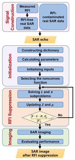
Figure 4.
The flowchart of the processing procedure.
3.4. The Proposed Adaptive Selection Scheme for Parameter
As previously described, WSVT is used for solving the subproblem, and the corresponding closed-form solution is represented in (17). In our DNLRM framework, the weighting function, , is substituted by the supergradients of different nonconvex functions. As for the mentioned supergradients, there are two influential parameters, and . The former proportionably affects the weighted values, whereas the curvature of the weighting curve is determined by the latter. In general, to make the singular values belonging to the RFIs obtain a smaller penalty, and the ones corresponding to the useful signal simultaneously deserve the larger penalty, is chosen as 0.5 in our experiments for a proper and balanced performance. Once is chosen, the parameter will ultimately determine the multiples of the weighting functions. Recall the relationship shown in (18); the generalized soft-thresholding operator needs to compare with the -related threshold. If becomes, large to a certain extent, even the large singular values will be excessively punished. Such a situation can still lead to the over-punishment of RFIs. Conversely, if is so small that all the singular values cannot receive enough of a penalty, then there is less of a presence of a useful signal, which causes severe degradation to the imaging result. Therefore, the appropriate value of , determined by parameter , is crucial to the implementation of the proposed DNLRM method.
In considering these facts, a modified boxplot based adaptive selection scheme of parameter is proposed in the present paper, which can be regarded as an outlier detection problem. For outlier detection, the rule and Z-score method are based on the assumption that data obeys the normal distribution, but the actual data does not always fit the distribution as expected. Their criteria for judging the outliers are directly based on the mean value and the standard deviation of the data. However, both of them are of such small tolerance, that the outliers themselves can have a great impact on them. On the contrary, the boxplot merely depends on the actual data itself, without assuming whether the data obeys a particular distribution. The boxplot judges the outliers via the quartile and the inter quartile range (IQR), which are more robust [40], thus more effective in terms of identifying the outliers. According to [41], a boxplot consists of the maximum, minimum, upper quartile (), median (), and lower quartile (). The location of can be calculated as , where index stands for the quartile and represents the sequence length, namely the number of singular values in our RFI suppression mission. and are then similarly obtained. Subsequently, IQR is calculated by subtracting from , which denotes the main body of the sequence with the elements having similar values. Therefore, a value is detected as the outlier once it is larger than the threshold .
The above calculation is the traditional detection mode used for the boxplot-based outliers, which is not appropriate if directly introduced into our adaptive selection scheme. Therefore, we improved it to fit our RFI suppression mission. Recall that the core idea of the proposed DNLRM method is to obtain the weighted penalty for singular values via the supergradient of the nonconvex function. In order to make the supergradient weighted penalties work effectively, the penalty curve needs to reach the order of magnitude of the singular values. Fortunately, the parameter can be used to raise the weighted value proportionally, then the core problem becomes the determination of the appropriate proportion. As considered above, the threshold can be used to set the boundary to distinguish the strong RFIs. Based on this, we suggest extending the boundary along the decreasing direction of the singular values for better distinguishing the performance for two reasons. The first one lies in that the threshold only considers the extremely strong outliers, namely the strong RFIs, whereas the relatively weaker RFIs may fall into the acceptable interval, which require further identification by the threshold extension. The second one is closely related to the proposed DNLRM method. As shown in Figure 5, the orange curve represents the supergradient-based penalty curve with the threshold , where the small singular values are protected but the larger ones are still over punished. After the threshold extension, the intersection of the singular value curve and the orange curve moves down (see the yellow star), and the green penalty curve is obtained. Accordingly, the penalties for the large singular values are further reduced and sufficient punishment for the small ones is ensured simultaneously. Through the threshold extension, the phenomenon that singular values of relatively weaker RFIs diffuse into the ones belonging to the useful signal is also considered.
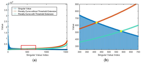
Figure 5.
Relationship between the weighted penalty curves and singular values. The blue curve represents the singular values, and the orange and the green ones, respectively represents the weighted penalty curve obtained by the boxplot without and with threshold extension. The curves in the red rectangle of (a) are enlarged to (b) for clearer vision.
Specifically, we recommend the following quantitative threshold extension scheme:
where and are the mean and the median of the singular values of . Both are calculated before performing WSVT (17). The rationality of the above scheme is twofold. First, represents the interval where the sequence values remain stable, so it can be considered as the proper baseline for threshold extension. The second one lies in that the ratio of the mean to the median, which can express the fluctuation of a sequence at a moderate level. Furthermore, as the signal-to-interference ratio (SIR) decreases, both of them become larger while the numerator changes more dramatically, hence the increasing ratio and the correspondingly more relaxed threshold shown in (25). Importantly, the concomitancy between SIR and the threshold is worth considering. When the RFI level increases, meaning a lower SIR, the singular values of relatively weaker RFIs become larger. This results in a more distinct diffusion, which demands a more relaxed threshold. Therefore, the statistics-based threshold extension (25) is needed to better adapt to the varying RFIs. Notice the enlarged area in Figure 5; the green curve obtained with a threshold extension, according to (25), is reduced appropriately compared with the orange one with no threshold extension. Correspondingly, the benefits are twofold. For the larger singular values, they further obtain a smaller penalty, and thus a better separation of strong RFIs. For the singular values slightly smaller than the intersection, they are fortunately reconsidered. The corresponding relatively weaker RFIs can be extracted from what will otherwise be pigeonholed to the useful signal. Finally, a transferring function, , is used to adjust the threshold, , for specific supergradient-based weighting functions to obtain the target parameter:
Recall (8): assuming that , we have for , and for . This can be accordingly generalized to other possible weighting functions.
The parameter obtained from the above modified boxplot is considered as the initial value for the subsequent adaptive fine search, to finally obtain the optimal . Specifically, based on the obtained initial value, , the step size for the adaptive fine search is chosen as one order of magnitude less than (i.e., /10). Firstly, take one positive step, obtaining , then obtain the corresponding metric and compare this with that of . The search will continue in the current direction if the obtained metric is better than that of the initial , otherwise the opposite direction will be pursued. Therefore, the search direction for the optimal value and the corresponding step size are obtained. Afterwards, the metric corresponding to the current obtained each time is compared with that of the last choice . If a better result is obtained, the search will continue for ; if worse, the last result of is considered as the better one. Successively, based on , and will be obtained with ±0.5 times the step size. Their corresponding metrics are then calculated and compared with that of to determine the final optimal parameter . Note that there is no human intervention needed in the entire searching process. Both the effectiveness and convenience of the adaptive selection scheme are reflected in the subsequent experiments.
4. Results
In this section, a series of experiments were conducted to verify the effectiveness and practicability of the proposed framework. First, we considered adding the measured RFI into the RFI-free real SAR data, which originally did not contain interference, to analyze the influence of different SIRs on several mentioned methods. Necessarily, the sparse scene and the dense scene were both considered to synthetically compare the RFI suppression performance. The sparse scenes refer to those imaging scenes with fewer scattering points, but containing obvious bright spots. On the contrary, those imaging scenes with relatively homogeneous and densely distributed scattering points were considered as dense scenes. In order to quantitatively evaluate the recovered images after RFI suppression, the normalized mean square error (NMSE) was used as the metric, which is formulated as:
where and are the imaging results, respectively, obtained from the original RFI-free real SAR data and the RFI suppression result when it was interfered with by RFIs. The images are generated via the imaging algorithm. As can be seen from the definition of NMSE, it considers the difference between the processed image and the reference one, so a smaller value represents a better RFI suppression performance. In addition, considering that the purpose of RFI suppression is to improve the image quality of the SAR image, both the image entropy and image contrast were also used to quantitatively analyze the image quality after RFI suppression. The image entropy is defined as:
where is the normalized histogram of the SAR image and is the gray level. Additionally, referring to [42], the image contrast can be modeled as:
where presents a certain point in the SAR image and denotes the mean value of the analyzed image. When an image becomes blurred due to the interference, the corresponding image entropy increases, indicating a worse image contrast. Accordingly, after RFI suppression, the image quality can be improved, which corresponds to a smaller image entropy and a larger image contrast. Subsequently, to further verify the performance of the proposed DNLRM method in the actual situation, experiments for suppressing the RFI-contaminated real SAR data were also carried out. The RFI-contaminated data means that RFIs were already contained in the received signal when collecting the data in real time, rather than the artificial combination of the RFI-free data with the measured RFI. The above two experimental configurations are the most realistic and referential ones, which provide a powerful illustration of the performance of different RFI suppression methods. Finally, the influence of the model parameter of the DNLRM method on RFI suppression performance was analyzed.
4.1. RFI-Free Real SAR Data with Measured RFI
To verify the outstanding performance of the proposed DNLRM method, sufficient experiments are conducted in this section. The RFI-free real SAR data was combined with the measured RFI to generate the interfered data for analysis. Meanwhile, the power of RFI was adjusted appropriately so that SIR, respectively, reached −20 dB, −15 dB, and −10 dB. Moreover, for a more comprehensive analysis of the RFI suppression performance, both the sparse scene and the dense scene with the figure size of 1536 × 2048 were under consideration. The specific parameters related to the RFI-free real SAR data are listed in Table 1, which are from the RADARSAT-1 SAR system.

Table 1.
Parameters related to the RFI-free real SAR data.
4.1.1. RFI Suppression Analysis for the Sparse Scene
In this section, the influence of RFI on sparse scene is analyzed, and the performance of the different RFI suppression methods is compared. Figure 6a illustrates the RFI-free SAR imaging result with the range and azimuth, respectively, lying along the horizontal direction and vertical one. The scene of the port and several ships is clearly visible, and so are the enlarged parts. Once RFI with a certain SIR, −20 dB here, is added to the RFI-free data, the imaging result is shrouded by the misty streaks, making the target scene completely unrecognizable, as shown in Figure 6b. To mitigate the effects of RFI, several methods, namely the NF method, ESP method, RNN method, DLRM method, the proposed DNLRM method with the nonconvex function selected as and , and the corresponding ADNLRM method, are used for the performance comparison. Note that the hyperparameters and not only act as tradeoff factors, but also participate in calculating the penalty. Therefore, both play an important part in the implementation of the optimization related methods, including our proposed method. In our experiments, and are, respectively, chosen as and according to [20]. Moreover, and are, respectively, 1.2 and 1 × 10⁶.
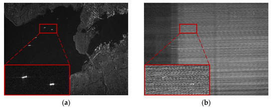
Figure 6.
Sparse scene: imaging results of (a) RFI-free real SAR data and (b) SAR data interfered by measured RFI. The size of the figures is 1536 × 2048.
Taking the case of −20 dB SIR as the example, detailed comparisons are analyzed as below. After being processed by the NF method, there are not only spectrum fractures, but also a large amount of remaining RFI sidelobes, which still leaves the imaging result blurred in severe RFI remnants, as shown in Figure 7c. The ESP method suppressed the RFI by constructing the RFI subspace, onto where the received signal was projected to separate RFI from the useful signal. Due to the fact that RFIs are a combination of many components with varying amplitudes, the subspace is often difficult to accurately classify. The orthogonality of subspace is consequently difficult to guarantee, which causes distinct streaks, shown in Figure 7d, due to the residual RFI. Figure 7e, processed via the RNN method, illustrates a large performance improvement compared with the first two. The low-rank property of RFI is exploited and the over-punishment problem is also considered by introducing the weighted penalty associated with the reciprocal of singular values, whereas in the RNN method, the non-sparse useful signal is directly used as the sparse regularization. The insufficient protection of the useful signal leads to the serious trailing of the imaging targets, as clearly shown in the enlarged area in Figure 8e, which still leaves room for performance improvement. On the contrary, the DLRM method intelligently uses the over-completed dictionary, in which the useful signal has a sparser representation, and the corresponding sparse coefficients are employed for regularizing the useful signal. Unfortunately, the over-punishment problem is not considered and the singular values are treated with the same penalty when updating low-rank matrices. As a result, parts of the RFIs are decomposed into the useful signal matrix, resulting in the imaging result shrouded in the noise-like residual RFIs, as shown in Figure 7f. In Figure 7g, the proposed DNLRM method reveals a superior RFI suppression performance with few RFI remnants and higher signal fidelity. The reason lies in the fact that the proposed DNLRM method simultaneously considers the appropriate sparse regularization with the usage of the over-completed dictionary and the more reasonable punishment scheme for the singular values. Here, larger singular values are treated with smaller penalties via the supergradient of the chosen nonconvex function. Furthermore, Figure 7g,h display a similar performance, and it is difficult to tell the difference using the naked eye. This is because their processing flows are both based on the proposed DNLRM method, except for choosing different nonconvex functions. Specifically, Figure 7g is obtained with , thus -DNLRM, and Figure 7h is obtained with , thus -DNLRM. The negative correlation between the supergradient and the singular values guarantees the small penalties of the large singular values, which ensures fewer RFI remnants. Further, the results of the proposed adaptive selection scheme shown in Figure 7i,j are, respectively, based on and , thus the -ADNLRM and the -ADNLRM. In addition to the superior RFI suppression performance, the trailing phenomenon is accordingly reduced, which can be clearly seen from the enlarged figures in Figure 8. Moreover, compared with DNLRM using the corresponding nonconvex function, ADNLRM can also achieve considerable performance while no human intervention is needed for searching parameter . This facilitates the adaptation to varying RFI suppression tasks. To observe the difference more clearly, the area within the red rectangle in Figure 7 is zoomed in to the corresponding position in Figure 8. The quantitative comparison of RFI suppression performance is listed in Table 2, Table 3 and Table 4. After a comprehensive evaluation, the proposed method achieves satisfactory performance improvement.
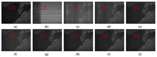
Figure 7.
Sparse scene: imaging results with SIR being −20 dB. Both (a,b) are the imaging results acquired by the RFI-free real SAR data before and after being interfered with by the measured RFI, respectively. The imaging results after RFI suppression are obtained with (c) the NF method, (d) the ESP method, (e) the RNN method, (f) the DLRM method, (g) the -DNLRM method, (h) the -DNLRM method, (i) the -ADNLRM method, and (j) the -ADNLRM method.
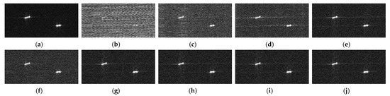
Figure 8.
Sparse scene: imaging results of the corresponding enlarged area in Figure 7 with SIR being −20 dB.
Table 2.
Sparse scene: NMSEs under different SIRs with various methods.
Table 3.
Sparse scene: image entropy under different SIRs with various methods.
Table 4.
Sparse scene: image contrast under different SIRs with various methods.
4.1.2. RFI Suppression Analysis for the Dense Scene
Comparative experiments for the dense scene are considered here. The imaging result of the RFI-free data shown in Figure 9a,b illustrates the image when it’s contaminated by RFI with the SIR being adjusted to −20 dB. The size of the figures is 1536 × 2048. Due to the presence of strong RFIs, the texture information of the target city area is completely invisible. The enlarged area, which is originally an area of water, only presents the severe RFI stripes after being contaminated.

Figure 9.
Dense scene: imaging results of (a) RFI-free real SAR data and (b) SAR data interfered by measured RFI. The size of the figures is 1536 × 2048.
For RFI mitigation, the methods and parameter configurations mentioned earlier in the sparse scene are used here. The −20 dB case shown in Figure 10 is used as the example for a detailed analysis, and the area within the red rectangle is enlarged in Figure 11. By comparison, it is obvious that there are still many streaks left in the imaging results after the use of the traditional NF and ESP methods. The NF method can suppress parts of obvious RFI with greater power, but fails to deal with the complex interferences. As a result, as shown in Figure 10c, the imaging result is still covered by severe RFI. As for the ESP method, the subspace is firstly constructed based on the RFI-contaminated received signal. Then, based on the amplitude difference in the singular values, respectively, corresponding to the RFI and useful signals, the separation of their subspaces is completed. However, the complexity and diversity of RFI makes it difficult to achieve an accurate subspace separation, resulting in the inevitable RFI remnants shown in Figure 10d. Furthermore, the optimization-based RNN method and DLRM method have made some improvements, but so not solve the problem of insufficient RFI suppression due to their respective inaccurate regularization. The former RNN method considers the low-rank property of RFI for the signal description on one hand; on the other hand, the weighted penalty is also employed by means of the reciprocal of singular values. Nevertheless, noise-like and non-sparse nature of the useful signal are not given proper consideration. As shown in Figure 10e, the direct usage of the non-sparse useful signal, as the sparse regularization leaves it, is in need of further optimization. For the latter DLRM method, the over-completed dictionary was considered to ensure the useful signal a sparser expression. Unfortunately, the SVT algorithm with the constant penalty was used to solve the low-rank minimization issue. The neglected improper punishment problem leads to parts of the RFIs being left in the useful signal, which results in the image still being surrounded by the noise-like RFIs, as illustrated in Figure 10f. Conversely, because both the appropriate selection of sparse regular and the logical punishment of the singular values are concurrently taken into account, the proposed DNLRM method achieves a considerably improved performance. Respectively obtained with the nonconvex functions of and , Figure 10g,h obtained a more sufficient RFI suppression performance while properly protecting the useful signals. Moreover, benefiting from the proposed adaptive searching scheme for , the considerable performance of DNLRM can be automatically obtained by ADNLRM, where the parameter searching process requires no human participation. Notably, this is true in both cases of the nonconvex function and , which verifies the robustness of the ADNLRM and is revealed in Figure 10i,j, respectively, with -ADNLRM and -ADNLRM. The above performance comparisons are shown in greater detail in the enlarged view in Figure 11. As can be observed in Figure 11, the outline of the area of water gradually emerges with the improving performance, and the noise in the dark area accordingly decreases. Among all the mentioned methods, the -ADNLRM method achieves the most outstanding RFI suppression result, as shown in Figure 11j, which is closest to the ground truth. It is worth noting that the scatterers in the dense scene are more densely distributed than those in the sparse scene, thus presenting a more severe influence on each other in the optimization process. For a quantitative analysis, see Table 5, Table 6 and Table 7. In a comprehensive view, the proposed method is verified to be superior.
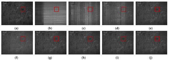
Figure 10.
Dense scene: imaging results with SIR being −20 dB. Both (a,b) are the imaging results acquired by the RFI-free real SAR data before and after being interfered with by the measured RFI, respectively. The imaging results after RFI suppression are obtained with (c) the NF method, (d) the ESP method, (e) the RNN method, (f) the DLRM method, (g) the -DNLRM method, (h) the -DNLRM method, (i) the -ADNLRM method, and (j) the -ADNLRM method.
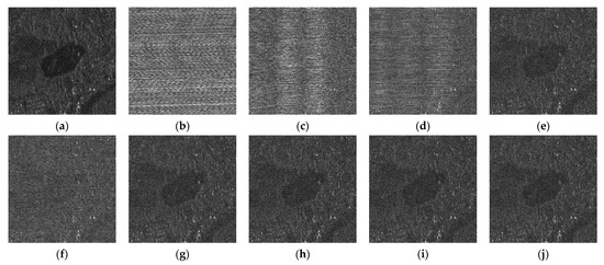
Figure 11.
Dense scene: imaging results of the corresponding enlarged area in Figure 10 with SIR being −20 dB.
Table 5.
Dense scene: NMSEs under different SIRs with various methods.
Table 6.
Dense scene: image entropy under different SIRs with various methods.
Table 7.
Dense scene: image contrast under different SIRs with various methods.
4.1.3. RFI Suppression Analysis against Different SIRs
In this section, the RFI suppression performance with various methods under different SIRs are analyzed. For the sparse scene, the quantitative metrics can refer to Table 2, Table 3 and Table 4. Similar comparisons for the dense scene are quantitatively shown in Table 5, Table 6 and Table 7. As the SIR decreases, the details of the imaging scene gradually deteriorate, and the SAR image is gradually dominated by RFI streaks leaving little valuable information. After performing RFI suppression with several methods, we obtain different levels of RFI suppression performance against the varying SIRs.
For the lateral comparison, comprehensively considering the evaluation results under the three metrics, namely NMSE, image entropy, and image contrast, the proposed method was verified to achieve a superior RFI suppression performance. Meanwhile, there were some detailed issues that need to be stated. Compared to the other mentioned methods, the performance improvement of DNLRM-related methods increased with the decrease in SIR. However, in a larger SIR, the advantages of the proposed method were not obvious enough. Taking RNN as the example, the reasons can be explained in the following three aspects. Firstly, due to the direct usage of the non-sparse useful signal as the sparse regularization in the RNN method, distortion correspondingly occurs in the recovered useful signal, and certain jitters appear in the spectrum. Larger SIR, for instance −10 dB, corresponded to the moderate interference, the spectrum of the processed signal was thereby less affected when suppressing RFI, and the influence of RNN processing on the recovered signal was relatively smaller. As the SIR worsened, the received signal was covered by more severe RFI, and its overall spectrum was increasingly affected. When pursuing a more adequate suppression of severe RFI, the signal spectrum will also be more seriously damaged due to the direct usage of the non-sparse useful signal in RNN, which brings nonnegligible errors to the recovered useful signal. Secondly, for moderate RFI, there were fewer large singular values diffusing into the ones that belonged to the useful signal. The RFIs were therefore easier to distinguish from the useful signal, even though the useful signal was not in its sparser form in the RNN. Finally, the core consideration in RFI suppression was to suppress the RFI as much as possible on the premise of protecting useful signals. However, the measured RFI signal was a mixture of interference signals and other noise signals obtained from the actual complex electromagnetic environment, which contained RFI with less low-rank properties and uncontrollable noise. These uncontrollable factors correspondingly influence the performance of RFI suppression. Additionally, although DLRM can achieve lower image entropy in larger SIR, the other two metrics are obviously worse than the proposed method, and the visual effect of the RFI suppression result using the DLRM method is also inferior. These results are due to the improper punishment problem caused by the usage of the constant penalty in DLRM. Furthermore, ADNLRM can achieve a similar considerable performance as DNLRM. Meanwhile, considering the advantage of not requiring human intervention, ADNLRM is more practical and suitable for the actual variable RFI environment.
For a longitudinal comparison, the three employed metrics showed a general trend of gradual deterioration with the decline in SIR, and there are two reasons accounting for this phenomenon. On one hand, the signal obtained in the listen-only mode was actually the combination of RFIs and the noise from the real-time working environment. With the decrease in the SIR, the noise accordingly increased, making the image after the RFI suppression still different from the original RFI-free imaging result. On the other hand, notice the fact that the measured RFI was a mixture of various forms of interference in practice, which was possibly not strictly low-rank. This caused the diffusing of larger singular values along the decreasing direction, making the low-rank decomposition more challenging, and, thus, the RFI remnants. Consequently, for the decreasing SIR, the energy of the residual RFIs and noise gradually increased. The difference between the original image and the RFI suppression result was accordingly expanded, hence the worse metrics. Notably, review Figure 5 that shows the threshold extension for the diffusion effect; the RFIs not being strictly low-rank was partly taken into account in the proposed ADNLRM method. The superiority lying in the implementation principle of ADNLRM method ensured its RFI suppression performance. The above laws are applicable to both the sparse case and the dense case. Furthermore, overall, the latter presented a worse performance for the more serious interactions of the densely distributed scatterers.
4.2. RFI-Contaminated Real SAR Data
In order to further verify the practicability of the proposed method, the experiments based on the RFI-contaminated real SAR data are analyzed here. Unlike the previous case, the RFI-contaminated data means that the SAR signal was already contaminated by the RFIs when receiving the echoes, rather than the combination of the RFI-free data with the measured RFI. Such a situation represents the most realistic electromagnetic environment. The RFI-contaminated SAR data was acquired via a P-band airborne SAR system from the Aerospace Information Research Institute of Chinese Academy of Sciences, with the system parameters listed in Table 8. In reality, there were many wireless communication devices operating within the frequencies around P-band. Once an SAR system is affected by the electromagnetic interference, there are severe RFI streaks overlaying the imaging result, as shown in Figure 12a, making it difficult to distinguish the scene information, let alone the subsequent operations. The size of the imaging result is 1638 × 4096. Notably, there is a large difference in the range resolution and azimuth resolution, and to make the height-to-width ratio of the imaging results closer to the actual scene, the figures have been reduced by 0.4 times in azimuth.
Table 8.
Parameters of the P-band airborne SAR system.
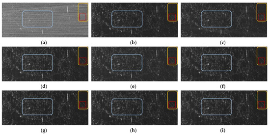
Figure 12.
Performance comparison of the different methods for the RFI-contaminated real SAR data. (a) is the imaging result acquired by the RFI-contaminated real SAR data, with a size of 1638 × 4096. The imaging results after RFI suppression are obtained with (b) the NF method, (c) the ESP method, (d) the RNN method, (e) the DLRM method, (f) the -DNLRM method, (g) the -DNLRM method, (h) the -ADNLRM method, and (i) the -ADNLRM method.
Note that there was no access to the original clean data for the RFI-contaminated case, thereby NMSE couldn’t be considered for the performance evaluation, in the present study. Instead, the metric of the ratio of signal-to-noise (SNR) was used for an effective evaluation. Specifically, for the RFI suppression results, the energy of the dark background with less scattering information (marked by a yellow rectangle in Figure 12) is chosen as the measurement of the noise, while the useful signal is measured by the energy of the intercepted feature-rich area (marked by a blue rectangle in Figure 12). Calculating the energy in the form of variance, SNR is defined as:
where and respectively represent the variance of the selected useful signal region and the noise area. Clearly, a larger SNR means less residual interference energy, thus a better RFI suppression result. Meanwhile, image entropy and image contrast were also considered to analyze the image quality. After RFI suppression, the improved image quality indicated corresponding smaller image entropy and larger image contrast.
To obtain the original appearance of the contaminated SAR image, a series of methods were used for suppressing RFIs with the corresponding performance shown in Figure 12. For a clearer visual comparison, the area marked in a red rectangle is enlarged in Figure 13. After being processed by the NF method and the ESP method, the imaging results can present the outline of the target scene, but with nonnegligible RFI remnants and noise. The improved imaging result is obtained via the RNN method, but there are still residual RFI streaks, as can be seen in Figure 13d. Additionally, the imaging result in Figure 13e appears to be shrouded in noise-like residual RFIs, which was obtained by the DLRM method associated with the improper punishment problem. Furthermore, as shown in Figure 13f,g, the imaging results, which are, respectively, obtained via the proposed -DNLRM and -DNLRM, demonstrate further improvements to the performance with fewer RFI streaks and noises. Finally, based on the introduced adaptive scheme, the optimal performance were automatically obtained. Figure 13h,i illustrate the RFI suppression results via -ADNLRM and -ADNLRM, respectively. The above experiments demonstrated the effectiveness and superiority of the proposed method, even in the realistic environment. The quantitative performance analysis is shown in Table 9, showing that the proposed method has the optimal comprehensive performance.
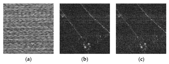
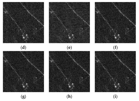
Figure 13.
Enlarged imaging results of the corresponding area are marked within the red rectangle in Figure 12. The size of the figures is 285 × 285.
Table 9.
Performance analysis for the RFI-contaminated real SAR data.
In addition, to illustrate the applicability of the proposed method to varying RFI suppression missions, another set of comparative experiments based on the RFI-contaminated real SAR data was carried out. The imaging results are shown in Figure 14 and enlarged to Figure 15, and the quantitative comparison is correspondingly listed in Table 10. The meanings of the marked boxes in Figure 14 are the same as those in Figure 12. The experimental results here have similar RFI suppression comparison results to the previous experiment, indicating that the proposed method can achieve a better RFI suppression performance and adapt to different RFI situations in reality, which further verifies its practicability.
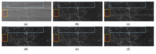
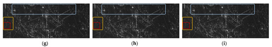
Figure 14.
Performance comparison of the different methods for the RFI-contaminated real SAR data. (a) is the imaging result acquired by the RFI-contaminated real SAR data, with a size of 1638 × 4096. The imaging results after RFI suppression are obtained with (b) the NF method, (c) the ESP method, (d) the RNN method, (e) the DLRM method, (f) the -DNLRM method, (g) the -DNLRM method, (h) the -ADNLRM method, and (i) the -ADNLRM method.
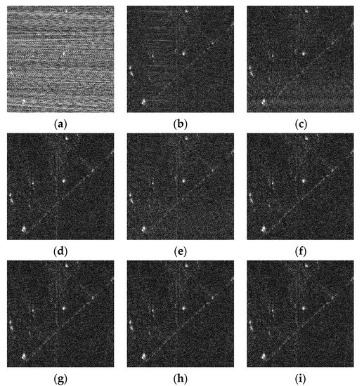
Figure 15.
Enlarged imaging results of the corresponding area marked within the red rectangle in Figure 14. The size of the figures is 285 × 285.
Table 10.
Performance analysis for the RFI-contaminated real SAR data.
4.3. Model Parameter Analysis
The regularity of parameter in the weighting function for affecting the RFI suppression performance is further unearthed in this section. The relationship between and NMSEs at different SIRs for the sparse scene is simulated and illustrated in Figure 16, where the noteworthy information is threefold. Firstly, for the optimal NMSE values of the three SIRs, they become worse with the deterioration of SIR. The reasons are clearly explained when analyzing the RFI suppression performance against the different SIRs evaluated earlier. Secondly, as the SIR decreases, the value of the optimal parameter marked by red arrows in Figure 16 concomitantly decreases. The reason for this is that a worse SIR means a more serious RFI, which increases the corresponding singular values belonging to the RFIs. To more thoroughly separate the RFIs from the useful signal, the penalty threshold must naturally be smaller for fewer RFI remains, thus a decreasing optimal parameter . Finally, the optimal performance is achieved only at the sole optimal parameter . There are two reasons accounting for this. The first is that when is small, the penalty for the useful signal is accordingly insufficient, namely the under-punishment of the useful signal. This results in the fact that part of the useful signal is divided into RFIs. As for the second reason, once increases to a certain extent, the over-punishment of large singular values occurs, thus the incomplete separation of RFIs. Both of them will cause a degradation to the image quality, leading to higher NMSEs. Without the loss of generality, the above regularities can fit in both and , which are, respectively, shown in Figure 16a,b. In addition, note that the selection of parameter is related to the target scene and the corresponding RFI level. Therefore, to make the DNLRM method more intelligent and practical, our adaptive scheme for parameter is further proposed, as described earlier.
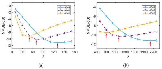
Figure 16.
Relationship between the parameter and NMSEs under different SIRs. The nonconvex function is, respectively, (a) and (b) .
5. Discussion
5.1. Convergence Analysis
In order to further verify the effectiveness of the proposed DNLRM framework, the convergence is theoretically analyzed here. The main idea of the proof is as follows, which is inspired by [30,31] and modified to specifically fit our optimization model. Firstly, prove that the sequence generated by the proposed DNLRM framework is bounded. Secondly, the Karush–Kuhn–Tucker (KKT) conditions are deduced to be satisfied. Finally, the accumulation point of the bounded sequence is proved to be the corresponding stationary point of the original problem. The specific derivation results can be seen in Appendix A.
5.2. Computational Complexity Analysis
In this section, the computational complexity of the mentioned optimization-based approaches is analyzed. Suppose that , then for the RNN algorithm [20], one SVD operation with , one vector inversion with , and one soft-thresholding operation with are needed. Therefore, the total computational complexity of the RNN algorithm is . As for the original dictionary-based low-rank minimization (DLRM) framework [17], it takes one SVD operation with , which is accompanied by one additional matrix multiplication related to the dictionary with to update the low-rank matrix. In addition, one soft-thresholding operation with is needed, which contains two additional matrix multiplications with to update the sparse matrix. Therefore, the total computational complexity reaches . The proposed DNLRM algorithm has the same computational complexity as the DLRM algorithm, except for one lightweight operation for calculating the weighed penalty with , so we obtain a total computational complexity with . As for the adaptive selection scheme, ADNLRM, it is implemented based on DNLRM. The modified boxplot-based threshold extension is first conducted to obtain the initial value, which is needed only once outside the loop. Then, in the fine searching process, the number of corresponding searches determines the final computational work, where the complexity of each attempt is the same as DNLRM. The related computational complexities are listed in Table 11. In summary, the proposed DNLRM algorithm effectively improves the RFI suppression performance at the cost of a lightweight increase in the computational complexity.
Table 11.
Comparison of computational complexity.
5.3. Relationship with Preceding Optimization Frameworks
Considering the priority of low rank, a series of optimization frameworks were proposed whereas, in most cases, the updating of low-rank RFI matrix was obtained via an SVT operation that treated all the singular values with the same penalty, thus resulting in the improper punishment. Moreover, the useful signal, which was noise-like and non-sparse, can also cause degradation to performance once directly used as the sparse regularization. To overcome these problems, the DNLRM framework was proposed in this paper by introducing the supergradient of the nonconvex function for calculating the weighted penalty. As a result, the larger singular values can be treated by correspondingly smaller penalties and vice versa. Here, we further emphasized the relationship and difference between the DNLRM framework and some preceding ones.
On one hand, when is ignored and the rank function is approximated by the function, namely with , the DNLRM framework degenerates to:
which represents the RNN algorithm. RNN considers the over-punishment problem, but the non-sparsity of the useful signal is not taken into account. The useful signal itself is directly used to act as sparse regularization, hence the restricted recovery performance. When the over-punishment problem is further ignored with , in other words, the rank function is approximated by the nuclear norm, then the DNLRM framework further degrades to
which is the classic RPCA form. When updating the low-rank matrix, the invariable penalty is considered via the SVT operation, which causes the improper punishment problem and the following incomplete RFI separation. On the other hand, if is considered but the rank function is still approximated by the nuclear norm, then the DNLRM framework converts back into the DLRM framework, that is:
where the improper punishment problem is likewise ignored.
Through the above analysis, as a result of simultaneously considering both the improper punishment problem and the non-sparsity of the useful signal, the proposed DNLRM framework outperforms the frameworks mentioned for comparison, especially in severe RFI situations. Compared with the preceding optimization methods mentioned in the manuscript, our method realizes the unification of them and further develops the strengths. Notably, this paper mainly focuses on the narrowband interference with a low rank, and there are two issues worth considering. For the first issue, although only narrowband interference was analyzed in this paper, the proposed method can also be used for effectively solving wideband interference once it satisfies the low-rank property. For the second issue, the RFI suppression performance was related to the degree to which the interference satisfied the low-rank property, regardless of being narrowband or wideband.
6. Conclusions
In this paper, a novel DNLRM method was proposed to more effectively suppress RFIs while guaranteeing the fidelity of the useful signal. Both the appropriate sparse regularization of the useful signal and the accurate low-rank approximation of RFIs were simultaneously considered. Innovatively, the advantages of the combined usage of the over-complete dictionary and the nonconvex approximating function were demonstrated theoretically and experimentally. Additionally, the mechanisms of over-punishment and under-punishment were analyzed adequately, and the corresponding solutions with appropriate penalties were provided. Subsequently, the role of weighted penalty based on the super-gradient in singular value punishment was revealed in detail. Afterwards, an adaptive selection scheme for the model parameter was proposed to adapt to different chosen nonconvex functions and the varying severity of RFIs, effectively and conveniently. Sufficient experiment results proved the superiority and practicability of the proposed method, especially those including the case of RFI-contaminated real SAR data, which reflected the most actual electromagnetic environment. Moreover, the proposed method was based on the low-rank assumption on RFI, whose degradation can affect the processing performance accordingly. Furthermore, as the dimension of the SAR data matrix increased, the computational efficiency of the algorithm could be gradually limited, which will be further studied in future work.
Author Contributions
Conceptualization, Z.T. and H.Z.; methodology, Z.T.; software, Z.T.; validation, Z.T.; formal analysis, Z.T. and H.Z.; investigation, Z.T. and H.Z.; resources, Y.D.; data curation, Y.D.; writing—original draft preparation, Z.T.; writing—review and editing, H.Z.; visualization, Z.T.; supervision, Y.D.; project administration, Y.D.; funding acquisition, Y.D. All authors have read and agreed to the published version of the manuscript.
Funding
This research was funded by the National Key Research and Development Program of China under Grant 2017YFB0502700.
Data Availability Statement
The analyzed data is not open access.
Acknowledgments
The authors would like to thank all reviewers and editors for their comments on this paper.
Conflicts of Interest
The authors declare no conflict of interest.
Appendix A. Convergence Analysis of the Proposed DNLRM Method
In Section 5.1, the main idea and detailed steps of convergence analysis for the proposed DNLRM method are presented, and the following is the specific proof process.
Lemma A1.
Lagrange multiplier sequence is bounded.
Proof of Lemma A1.
The augmented Lagrangian can be written as
Considering that is the optimal solution of the subproblem, satisfies the first order optimal condition, namely
Meanwhile, is bounded and is an over-completed dictionary constructed from the discrete time-shifted versions of the transmitted signal with a finite value, so is bounded.
Lemma A2.
When , the low-rank matrix sequence and the sparse matrix sequence are both bounded.
Proof of Lemma A2.
Based on the updating formulas shown in Section 3.2, the following derivation can be obtained:
Theorem A1.
Let be the sequence generated by the proposed DNLRM framework with being a corresponding accumulation point, then is a stationary point of the original problem once .
Proof of Theorem A1.
is bounded when , which is known from Lemma A1 and Lemma A2. Therefore
As is bounded, the following equation holds:
Moreover, is the optimal solution of the subproblem, therefore so that the following first order optimality condition holds:
Additionally, since the selected is nonconvex and , we obtain , where is nonconcave. Based on the nonconcave property of , consider the upper semi-continuous property of the subdifferential [43], then . Therefore, and converge to . Accordingly
Recall (A3) when proving Lemma A1, and review the relationship between the accumulation point and the corresponding sequence, from which we obtain:
To sum up, as shown in (A9), (A11), and (A12), the accumulation point meets the KKT condition related to the augmented Lagrangian function , so is a stationary point of the original problem (10). □
References
- Moreira, A.; Prats-Iraola, P.; Younis, M.; Krieger, G.; Hajnsek, I.; Papathanassiou, K.P. A tutorial on synthetic aperture radar. IEEE Geosci. Remote Sens. Mag. 2013, 1, 6–43. [Google Scholar] [CrossRef] [Green Version]
- Tang, Z.; Deng, Y.; Zheng, H.; Wang, R. High-Fidelity SAR Intermittent Sampling Deceptive Jamming Suppression Using Azimuth Phase Coding. IEEE Geosci. Remote Sens. Lett. 2021, 18, 489–493. [Google Scholar] [CrossRef]
- Tao, M.; Su, J.; Huang, Y.; Wang, L. Mitigation of Radio Frequency Interference in Synthetic Aperture Radar Data: Current Status and Future Trends. Remote Sens. 2019, 11, 2438. [Google Scholar] [CrossRef] [Green Version]
- Meyer, F.J.; Nicoll, J.B.; Doulgeris, A.P. Correction and Characterization of Radio Frequency Interference Signatures in L-Band Synthetic Aperture Radar Data. IEEE Trans. Geosci. Remote Sens. 2013, 51, 4961–4972. [Google Scholar] [CrossRef] [Green Version]
- Leng, X.; Ji, K.; Zhou, S.; Xing, X.; Zou, H. Discriminating Ship From Radio Frequency Interference Based on Noncircularity and Non-Gaussianity in Sentinel-1 SAR Imagery. IEEE Trans. Geosci. Remote Sens. 2019, 57, 352–363. [Google Scholar] [CrossRef]
- Natsuaki, R.; Motohka, T.; Watanabe, M.; Shimada, M.; Suzuki, S. An Autocorrelation-Based Radio Frequency Interference Detection and Removal Method in Azimuth-Frequency Domain for SAR Image. IEEE J. Sel. Top. Appl. Earth Observ. Remote Sens. 2017, 10, 5736–5751. [Google Scholar] [CrossRef]
- Chang, W.; Cherniakov, M.; Li, X.; Li, J. Performance analysis of the notch filter for RF Interference suppression in ultra-wideband SAR. In Proceedings of the 9th International Conference on Signal Processing, Beijing, China, 26–29 October 2008; pp. 2446–2451. [Google Scholar]
- Buckreuss, S.; Horn, R. E-SAR P-band SAR subsystem design and RF-interference suppression. In Proceedings of the 1998 IEEE International Geoscience and Remote Sensing Symposium, Seattle, WA, USA, 6–10 July 1998; pp. 466–468. [Google Scholar]
- Zhou, F.; Wu, R.; Xing, M.; Bao, Z. Eigensubspace-Based Filtering With Application in Narrow-Band Interference Suppression for SAR. IEEE Geosci. Remote Sens. Lett. 2007, 4, 75–79. [Google Scholar] [CrossRef]
- Yu, C.; Zhang, Y.; Dong, Z.; Liang, D. Eigen-Decomposition Method for RFI Suppression Applied to SAR Data. In Proceedings of the 2010 International Conference on Multimedia Technology, Ningbo, China, 29–31 October 2010; pp. 1–4. [Google Scholar]
- Lord, R.T.; Inggs, M.R. Approaches to RF interference suppression for VHF/UHF synthetic aperture radar. In Proceedings of the 1998 South African Symposium on Communications and Signal Processing, Rondebosch, South Africa, 8 September 1998; pp. 95–100. [Google Scholar]
- Le, C.T.C.; Hensley, S.; Chapin, E. Adaptive Filtering of RFI in Wideband SAR Signals. In Proceedings of the 1998 7th Airborne Geoscience Workshop, Pasadena, CA, USA, 12 January 1998; pp. 41–50. [Google Scholar]
- Lord, R.T.; Inggs, M.R. Efficient RFI suppression in SAR using a LMS adaptive filter with sidelobe suppression integrated with the range-Doppler algorithm. In Proceedings of the 1999 IEEE International Geoscience and Remote Sensing Symposium, Hamburg, Germany, 28 June–2 July 1999; pp. 574–576. [Google Scholar]
- Zhou, F.; Xing, M.; Bai, X.; Sun, G.; Bao, Z. Narrow-Band Interference Suppression for SAR Based on Complex Empirical Mode Decomposition. IEEE Geosci. Remote Sens. Lett. 2009, 6, 423–427. [Google Scholar] [CrossRef]
- Ojowu, O.; Li, J. RFI Suppression for Synchronous Impulse Reconstruction UWB Radar Using RELAX. Int. J. Remote Sens. Appl. 2013, 3, 33–46. [Google Scholar]
- Yang, Z.; Du, W.; Liu, Z.; Liao, G. WBI Suppression for SAR Using Iterative Adaptive Method. IEEE J. Sel. Top. Appl. Earth Observ. Remote Sens. 2016, 9, 1008–1014. [Google Scholar] [CrossRef]
- Nguyen, L.; Dao, M.; Tran, T. Radio-frequency interference separation and suppression from ultrawideband radar data via low-rank modeling. In Proceedings of the 2014 IEEE International Conference on Image Processing, Paris, France, 27–30 October 2014; pp. 116–120. [Google Scholar]
- Nguyen, L.; Tran, T. RFI-radar signal separation via simultaneous low-rank and sparse recovery. In Proceedings of the 2016 IEEE Radar Conference, Philadelphia, PA, USA, 2–6 May 2016; pp. 1–5. [Google Scholar]
- Huang, Y.; Liao, G.; Li, J.; Xu, J. Narrowband RFI Suppression for SAR System via Fast Implementation of Joint Sparsity and Low-Rank Property. IEEE Trans. Geosci. Remote Sens. 2018, 56, 2748–2761. [Google Scholar] [CrossRef]
- Huang, Y.; Liao, G.; Xiang, Y.; Zhang, Z.; Li, J.; Nehorai, A. Reweighted Nuclear Norm and Reweighted Frobenius Norm Minimizations for Narrowband RFI Suppression on SAR System. IEEE Trans. Geosci. Remote Sens. 2019, 57, 5949–5962. [Google Scholar] [CrossRef]
- Lu, X.; Yang, J.; Yu, W.; Su, W.; Gu, H.; Yeo, T.S. Enhanced LRR-Based RFI Suppression for SAR Imaging Using the Common Sparsity of Range Profiles for Accurate Signal Recovery. IEEE Trans. Geosci. Remote Sens. 2021, 59, 1302–1318. [Google Scholar] [CrossRef]
- Huang, Y.; Liao, G.; Xu, J.; Li, J. Narrowband RFI Suppression for SAR System via Efficient Parameter-Free Decomposition Algorithm. IEEE Trans. Geosci. Remote Sens. 2018, 56, 3311–3322. [Google Scholar] [CrossRef]
- Huang, Y.; Liao, G.; Zhang, Z.; Xiang, Y.; Li, J.; Nehorai, A. Fast Narrowband RFI Suppression Algorithms for SAR Systems via Matrix-Factorization Techniques. IEEE Trans. Geosci. Remote Sens. 2019, 57, 250–262. [Google Scholar] [CrossRef]
- Candès, E.J.; Li, X.D.; Ma, Y.; Wright, J. Robust principal component analysis? J. ACM 2011, 58, 11. [Google Scholar] [CrossRef]
- Bouwmans, T.; Javed, S.; Zhang, H.; Lin, Z.; Otazo, R. On the Applications of Robust PCA in Image and Video Processing. Proc. IEEE 2018, 106, 1427–1457. [Google Scholar] [CrossRef] [Green Version]
- Yan, H.; Wang, R.; Li, F.; Deng, Y.; Liu, Y. Ground Moving Target Extraction in a Multichannel Wide-Area Surveillance SAR/GMTI System via the Relaxed PCP. IEEE Geosci. Remote Sens. Lett. 2013, 10, 617–621. [Google Scholar] [CrossRef]
- Cai, J.-F.; Candès, E.J.; Shen, Z. A singular value thresholding algorithm for matrix completion. SIAM J. Optim. 2010, 20, 1956–1982. [Google Scholar] [CrossRef]
- Wright, J.; Ganesh, A.; Rao, S.; Peng, Y.; Ma, Y. Robust principal component analysis: Exact recovery of corrupted low-rank matrices via convex optimization. In Proceedings of the 23rd Annual Conference on Neural Information Processing Systems, Vancouver, BC, Canada, 7–10 December 2009; pp. 2080–2088. [Google Scholar]
- Liu, H.; Li, D.; Zhou, Y.; Truong, T.-K. Joint Wideband Interference Suppression and SAR Signal Recovery Based on Sparse Representations. IEEE Geosci. Remote Sens. Lett. 2017, 14, 1542–1546. [Google Scholar] [CrossRef]
- Lu, C.; Tang, J.; Yan, S.; Lin, Z. Nonconvex Nonsmooth Low Rank Minimization via Iteratively Reweighted Nuclear Norm. IEEE Trans. Image Process. 2016, 25, 829–839. [Google Scholar] [CrossRef] [PubMed] [Green Version]
- Chen, Y.; Guo, Y.; Wang, Y.; Wang, D.; Peng, C.; He, G. Denoising of Hyperspectral Images Using Nonconvex Low Rank Matrix Approximation. IEEE Trans. Geosci. Remote Sens. 2017, 55, 5366–5380. [Google Scholar] [CrossRef]
- Xie, T.; Li, S.; Sun, B. Hyperspectral Images Denoising via Nonconvex Regularized Low-Rank and Sparse Matrix Decomposition. IEEE Trans. Image Process. 2019, 29, 44–56. [Google Scholar] [CrossRef]
- Hu, Y.; Li, X.; Gu, Y.; Jacob, M. Hyperspectral Image Recovery Using Nonconvex Sparsity and Low-Rank Regularizations. IEEE Trans. Geosci. Remote Sens. 2020, 58, 532–545. [Google Scholar] [CrossRef]
- Nguyen, L.H.; Tran, T.; Do, T. Sparse models and sparse recovery for ultra-wideband SAR applications. IEEE Trans. Aerosp. Electron. Syst. 2014, 50, 940–958. [Google Scholar] [CrossRef]
- Boyd, S.; Parikh, N.; Chu, E.; Peleato, B.; Eckstein, J. Distributed optimization and statistical learning via the alternating direction method of multipliers. Found. Trends Mach. Learn. 2011, 3, 1–122. [Google Scholar] [CrossRef]
- Zhu, F.; Halimi, A.; Honeine, P.; Chen, B.; Zheng, N. Correntropy Maximization via ADMM: Application to Robust Hyperspectral Unmixing. IEEE Trans. Geosci. Remote Sens. 2017, 55, 4944–4955. [Google Scholar] [CrossRef] [Green Version]
- Gu, S.; Zhang, L.; Zuo, W.; Feng, X. Weighted Nuclear Norm Minimization with Application to Image Denoising. In Proceedings of the 2014 IEEE Conference on Computer Vision and Pattern Recognition, Columbus, OH, USA, 23–28 June 2014; pp. 2862–2869. [Google Scholar]
- Wright, S.J.; Nowak, R.D.; Figueiredo, M.A.T. Sparse Reconstruction by Separable Approximation. IEEE Trans. Signal Process. 2009, 57, 2479–2493. [Google Scholar] [CrossRef] [Green Version]
- Yang, J.; Yin, W.; Zhang, Y.; Wang, Y. A fast algorithm for edge-preserving variational multichannel image restoration. SIAM J. Imag. Sci. 2009, 2, 569–592. [Google Scholar] [CrossRef]
- Shevlyakov, G.; Andrea, K.; Choudur, L.; Smirnov, P.; Ulanov, A.; Vassilieva, N. Robust versions of the Tukey boxplot with their application to detection of outliers. In Proceedings of the 2013 IEEE International Conference on Acoustics, Speech and Signal Processing, Vancouver, BC, Canada, 26–31 May 2013; pp. 6506–6510. [Google Scholar]
- Zhang, C.; Li, G.; Cui, W. High resolution remote sensing image change detection based on law of cosines with box-whisker plot. In Proceedings of the 2017 International Workshop on Remote Sensing with Intelligent Processing, Shanghai, China, 18–21 May 2017; pp. 1–9. [Google Scholar]
- Zhang, S.; Xing, M.; Guo, R.; Zhang, L.; Bao, Z. Interference Suppression Algorithm for SAR Based on Time–Frequency Transform. IEEE Trans. Geosci. Remote Sens. 2011, 49, 3765–3779. [Google Scholar] [CrossRef]
- Clarke, F.H. Nonsmooth analysis and optimization. In Proceedings of the International Congress of Mathematicians, Helsinki, Finland, 7 October 1978; pp. 847–853. [Google Scholar]
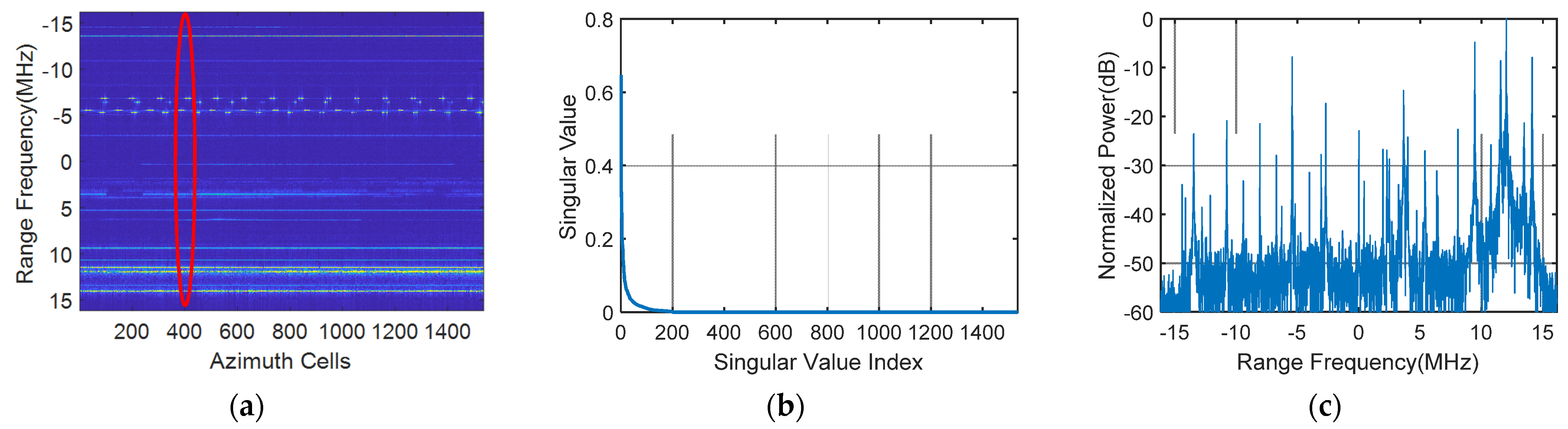

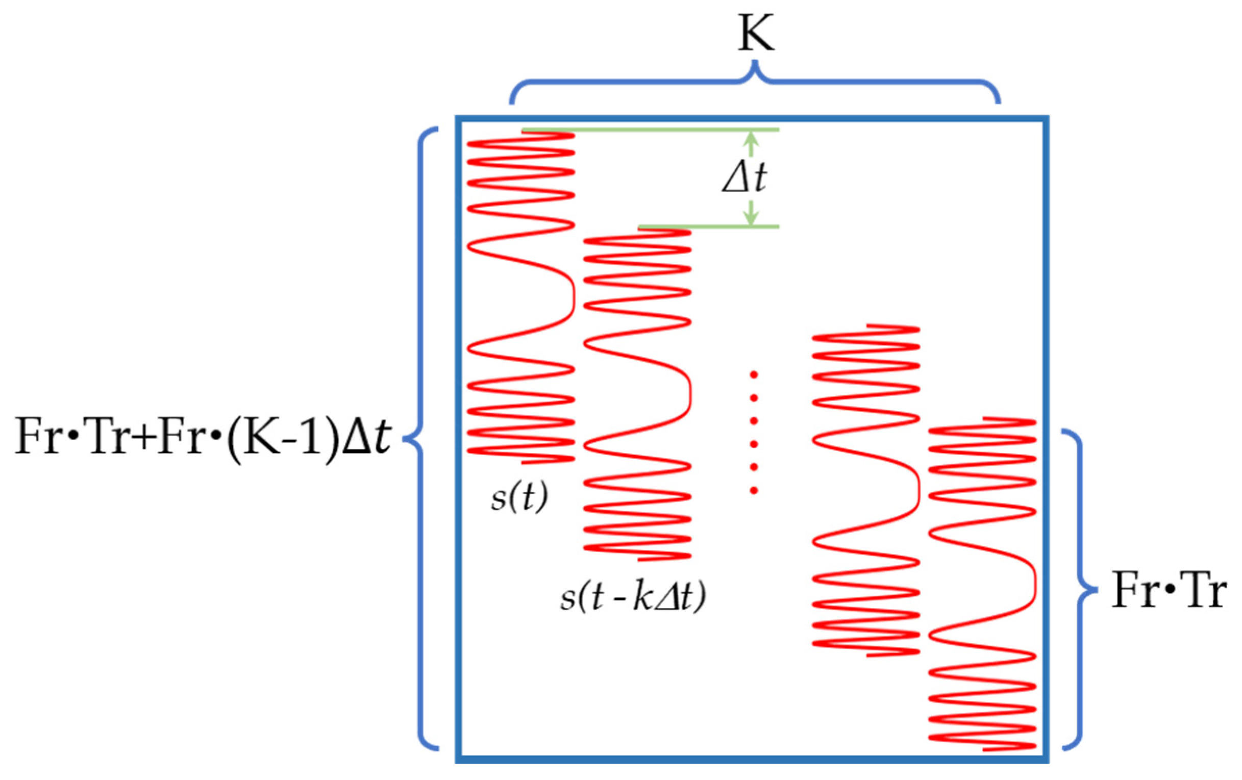

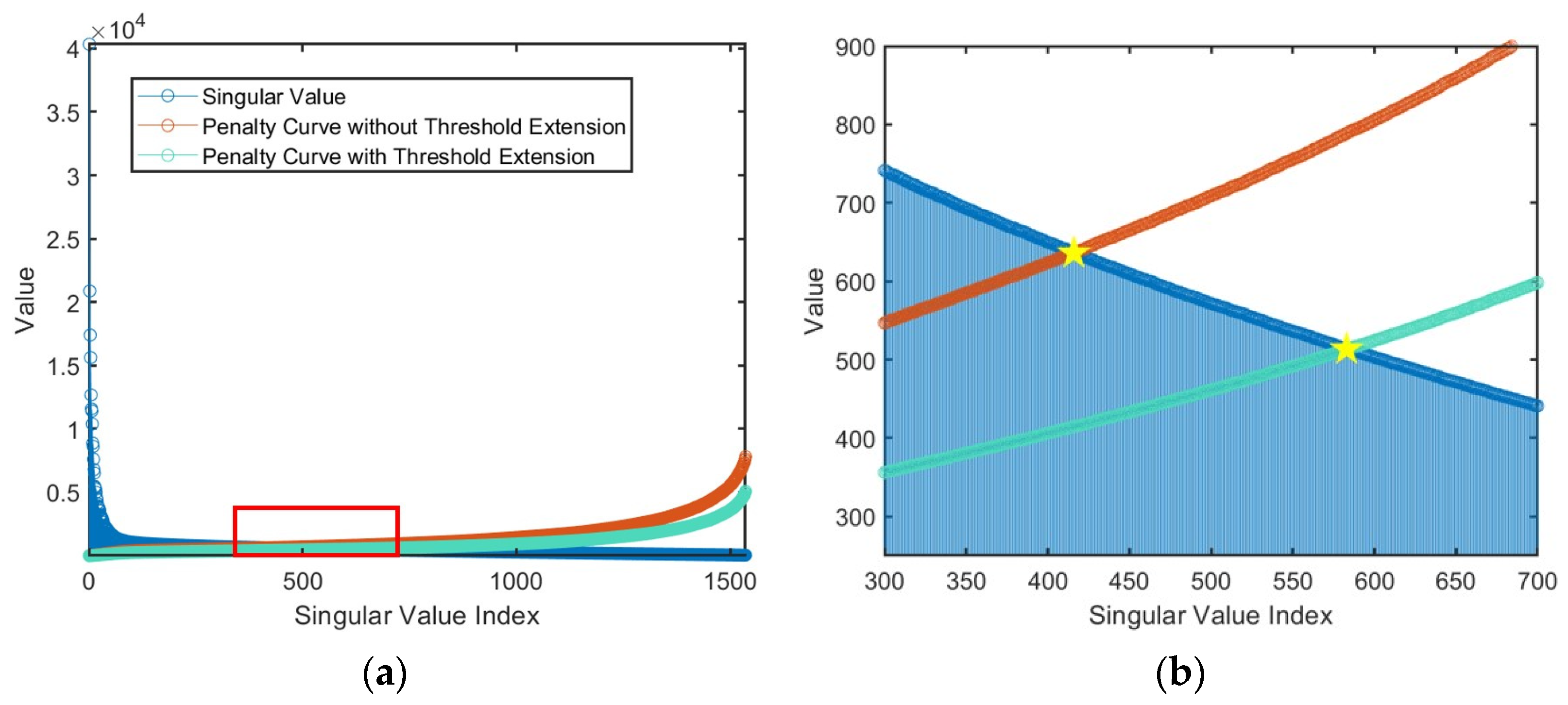
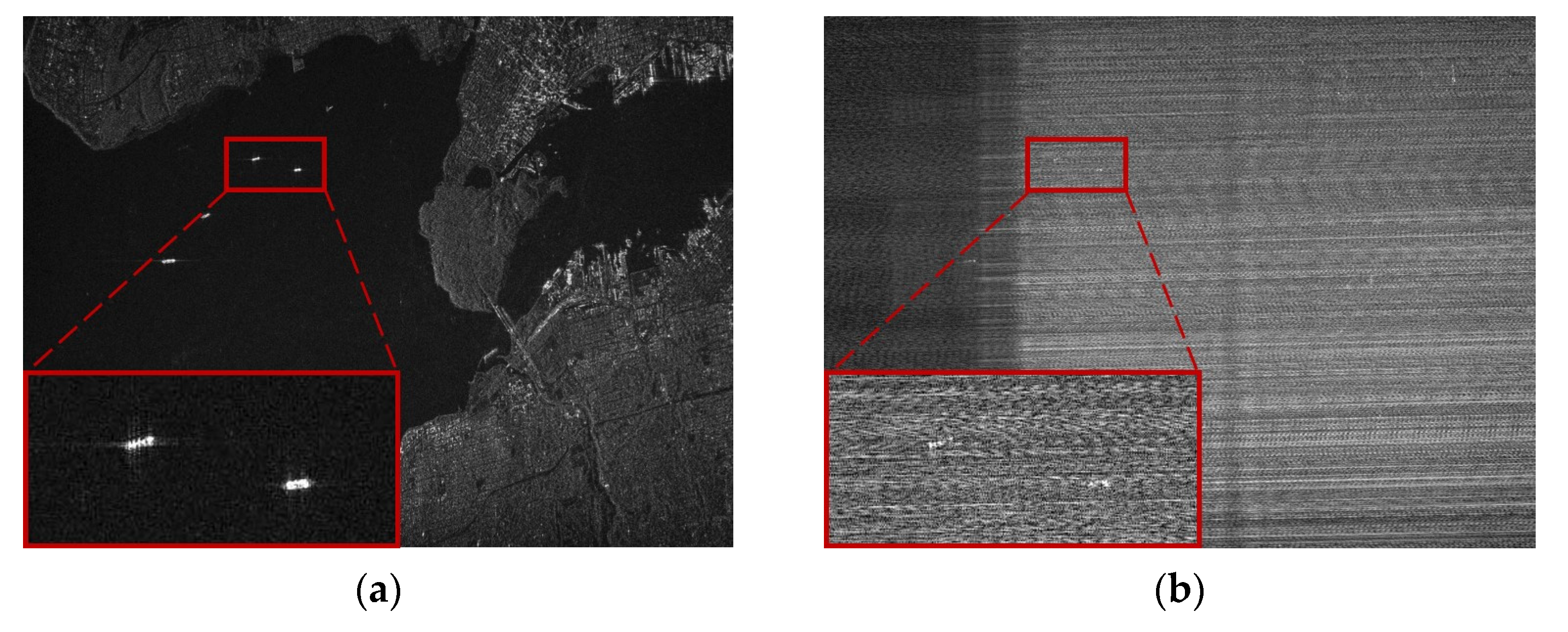
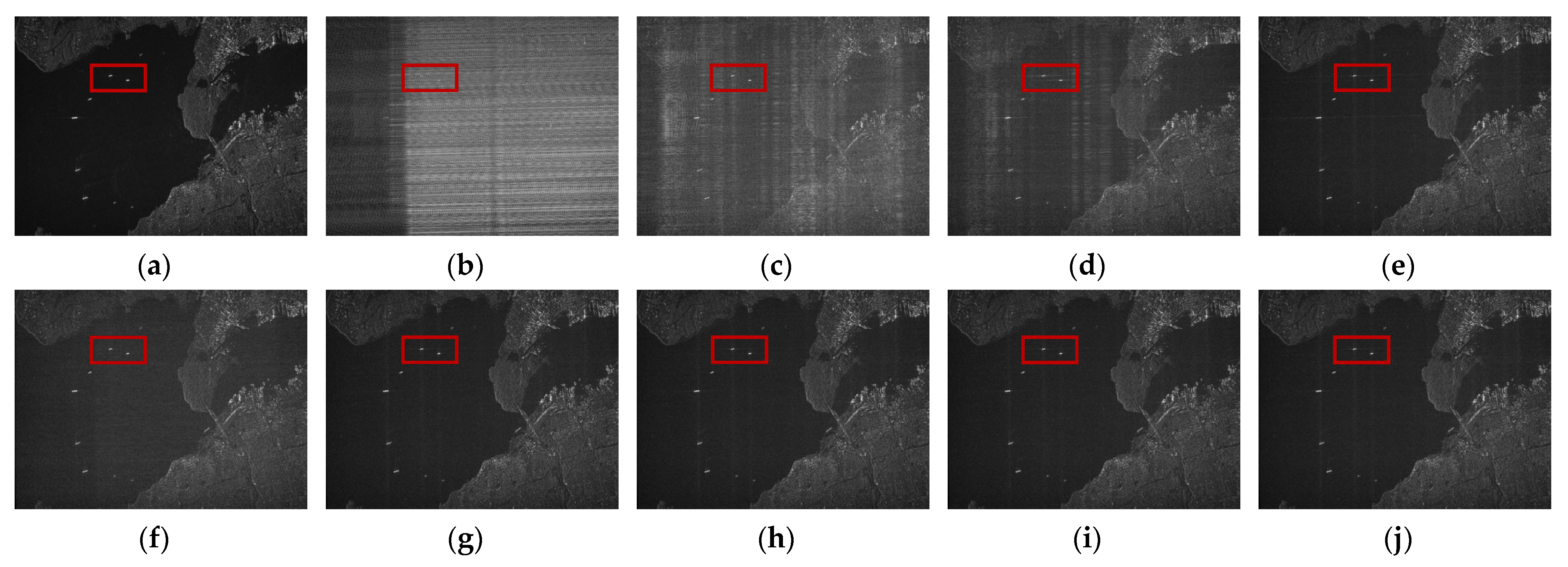
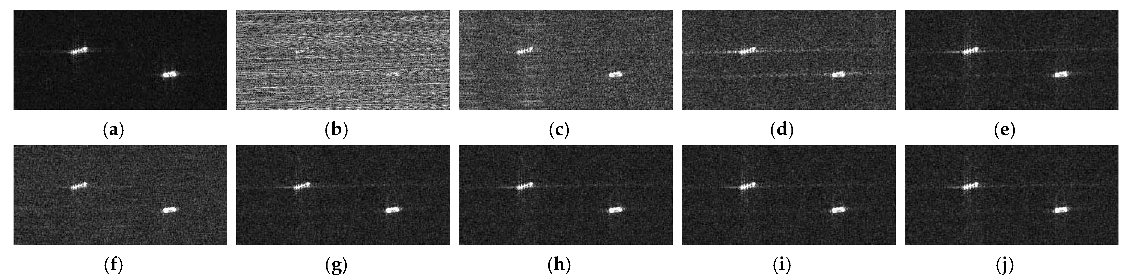
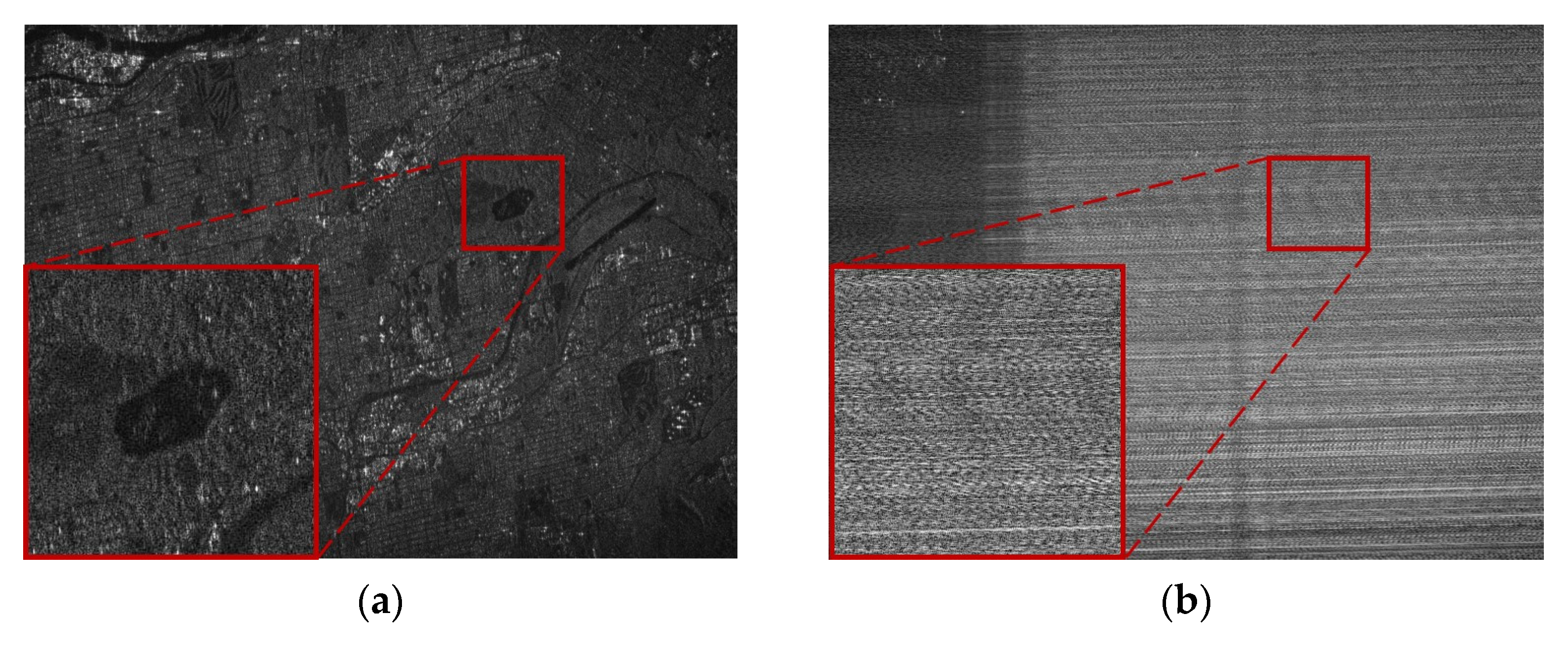
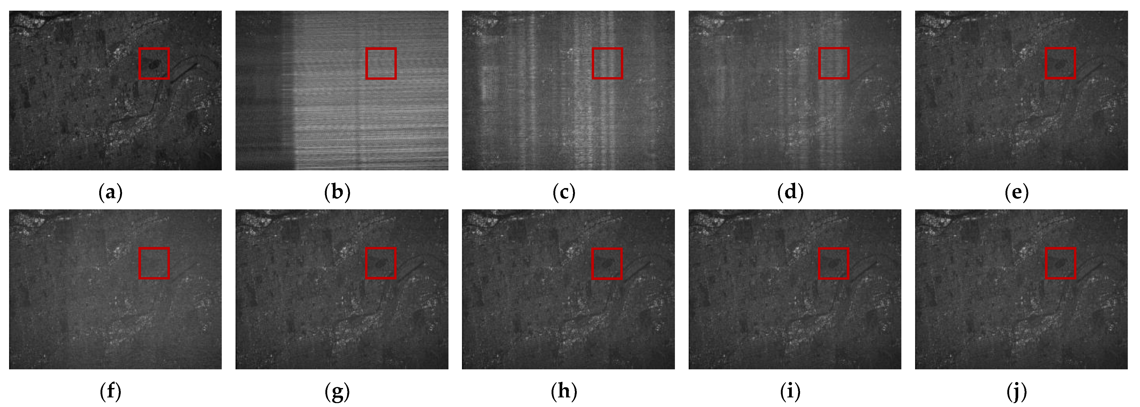
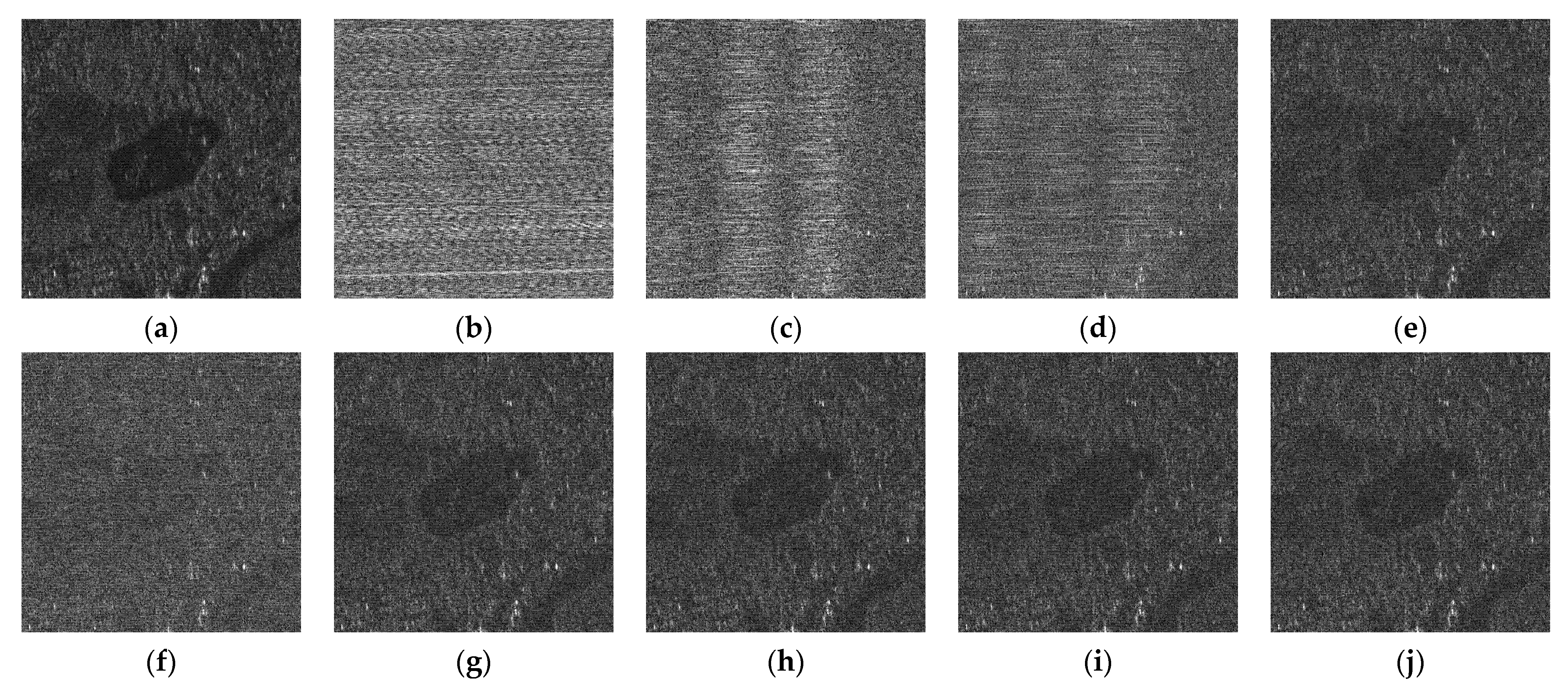
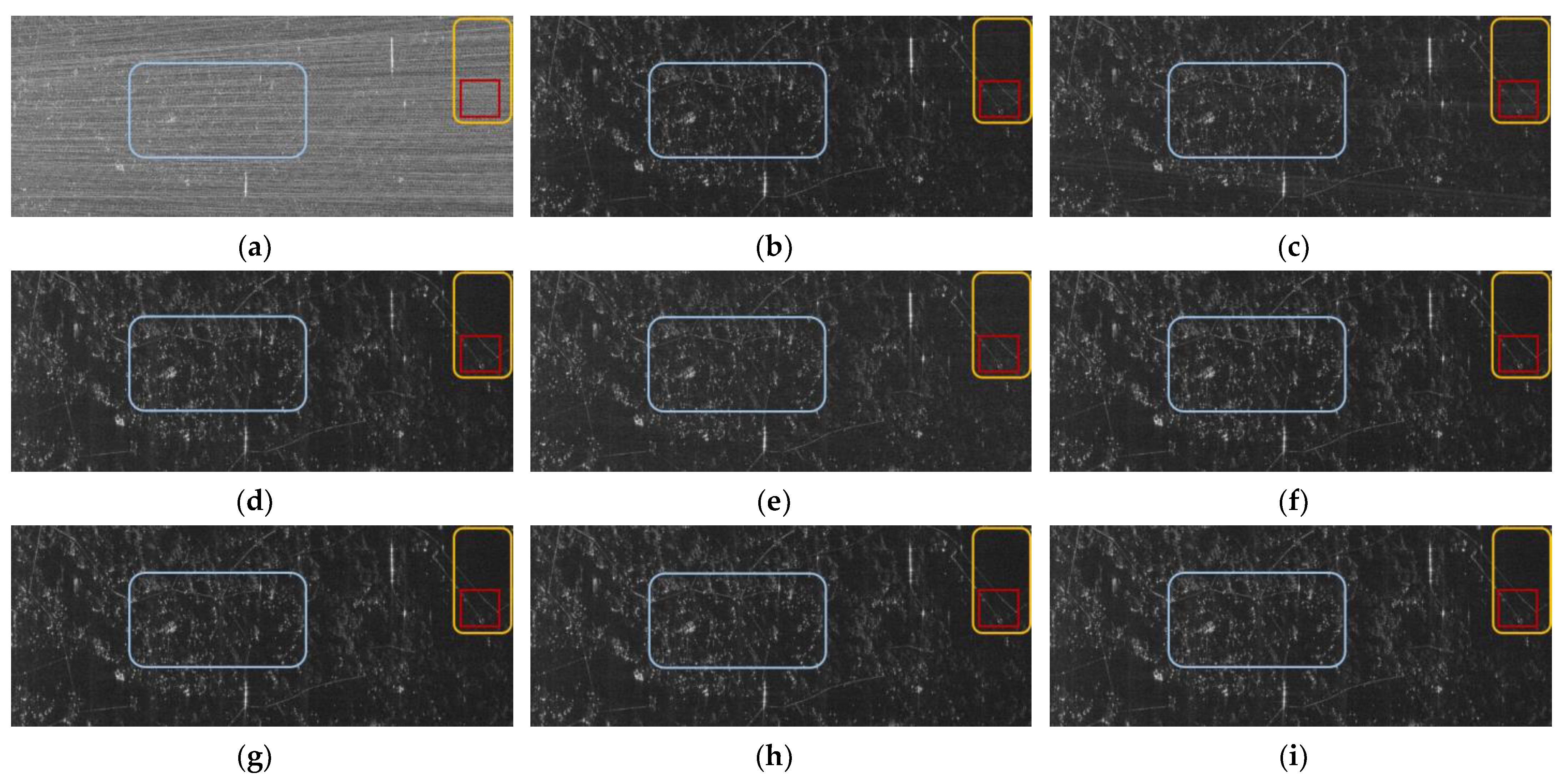
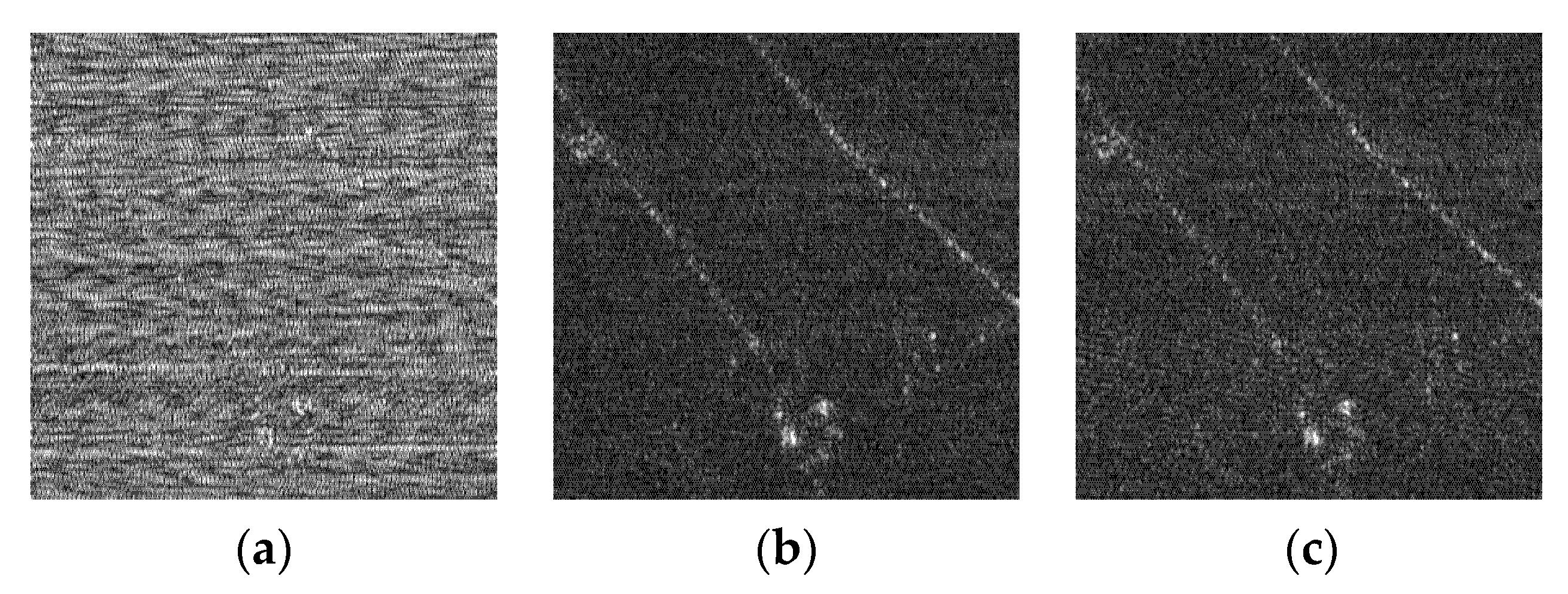
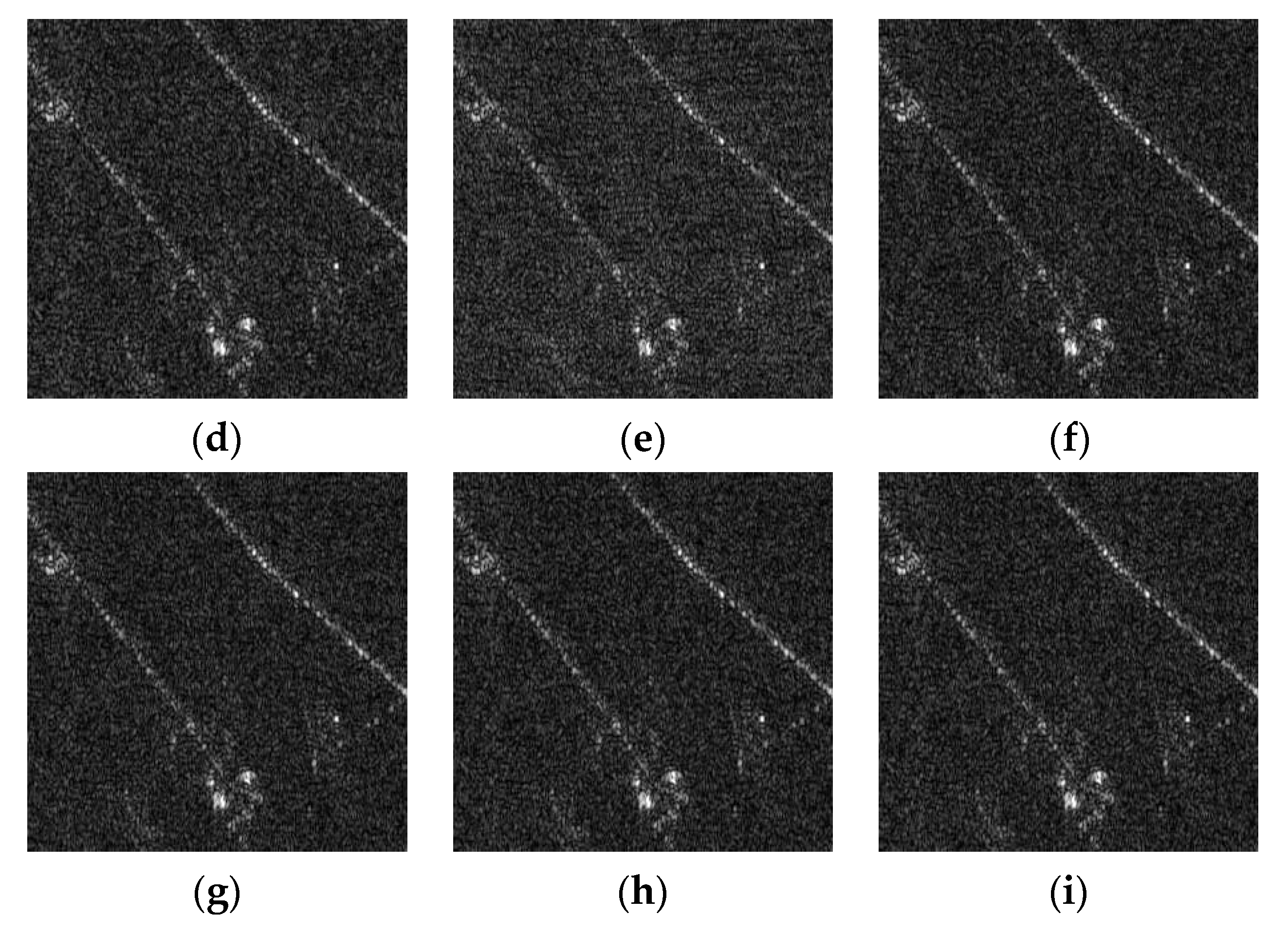
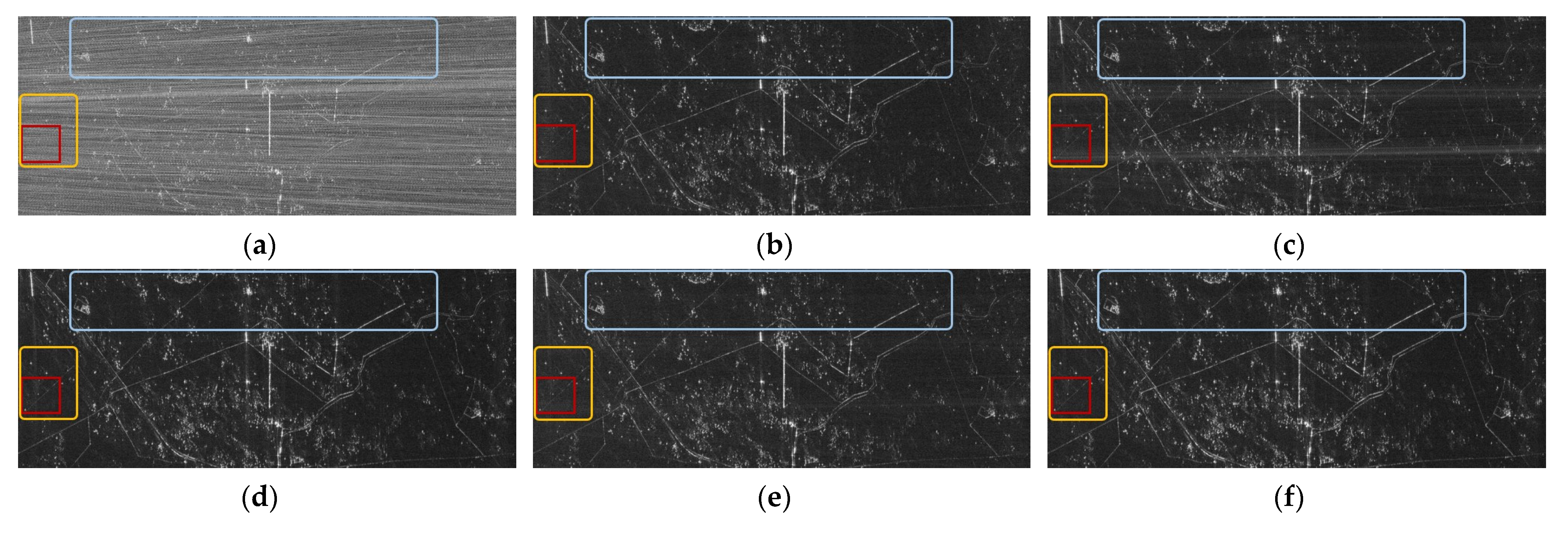
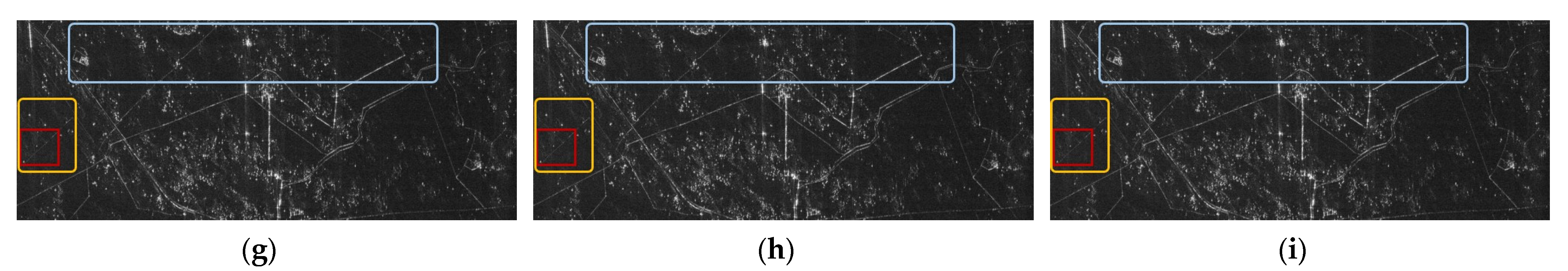
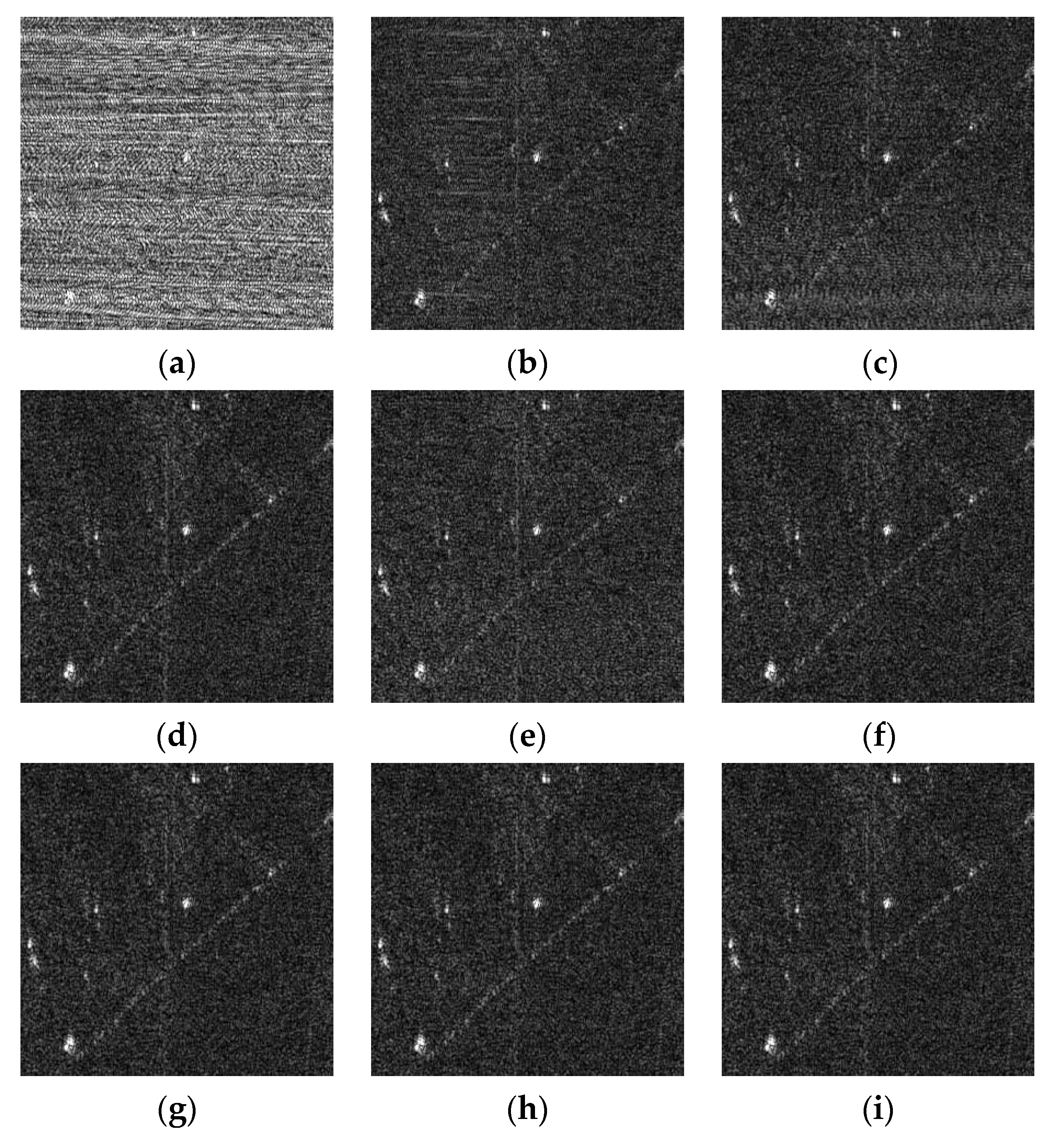

Publisher’s Note: MDPI stays neutral with regard to jurisdictional claims in published maps and institutional affiliations. |
© 2022 by the authors. Licensee MDPI, Basel, Switzerland. This article is an open access article distributed under the terms and conditions of the Creative Commons Attribution (CC BY) license (https://creativecommons.org/licenses/by/4.0/).