Abstract
Effective and precise monitoring is a prerequisite to control human emissions and slow disruptive climate change. To obtain the near-real-time status of power plant emissions, we built machine learning models and trained them on satellite observations (Sentinel 5), ground observed data (EPA eGRID), and meteorological observations (MERRA) to directly predict the NO2 emission rate of coal-fired power plants. A novel approach to preprocessing multiple data sources, coupled with multiple neural network models (RNN, LSTM), provided an automated way of predicting the number of emissions (NO2, SO2, CO, and others) produced by a single power plant. There are many challenges on overfitting and generalization to achieve a consistently accurate model simply depending on remote sensing data. This paper addresses the challenges using a combination of techniques, such as data washing, column shifting, feature sensitivity filtering, etc. It presents a groundbreaking case study on remotely monitoring global power plants from space in a cost-wise and timely manner to assist in tackling the worsening global climate.
1. Introduction
Man-made emissions are the main cause of global climate change and exert myriad impacts on environmental ecosystems and human well-being, including greater frequency and magnitude of disruptive climate events, such as exceptional drought, hurricanes, and deadly flash flooding. Action must be taken to stop the trends in the next decades to slow down the increase of global temperature which has already increased by 1.5 Celsius, on average, above pre-industrial levels, a rate which has not been seen in the past 2000 years. Many groups and world governments are taking steps to reduce emissions through precautionary short-term and long-term goals to fight the concerning change.
U.S. EPA (Environmental Protection Agency) reports that over a quarter of the total emissions of both pollutants and greenhouse gases in the United States come from the energy sector and the majority is from burning coal, fossil fuels, and natural gas. Power demand varies closely with the weather (especially extreme warmth and cold), which changes significantly over daily timescales.
An essential step to control emissions is to accurately monitor them on a timely basis to prevent further severe emission releases to the atmosphere. Currently, EPA requires coal-fired power plant facilities to install real-time sensors to their emission outlets, such as chimneys, and to send the data back regularly. The data is accurate and continuous and serves as the sole source of information for policymaking and emissions control. However, ground observation is expensive to install and maintain and only power plants in the United States and some western countries allow open access to their high-resolution data so far. To manage global emissions as a whole, we should have the ability to monitor all the power plants around the world at low cost and in an environment-friendly manner.
EPA currently regulates nitrogen dioxide (NO2), the most important member in the NOx family in the troposphere. NO2 can react and create ozone (O3). EPA defined national ambient air quality standards (NAAQS) to regulate tropospheric NO2 levels for the sake of public health. The recommended safe threshold of annual arithmetic mean concentration is 0.053 parts per million (ppm) (100 micrograms per cubic meter) [1]. Power plants are one of the main sources of human-induced NO2 due to their coal/gas combustion. One of three chemical mechanisms results in the formation of NOx: (1) “thermal” NOx, which accounts for 75% of NOx, is produced by oxidation of molecular nitrogen by combustion in air; (2) “fuel” NOx, which accounts for 20% of NOx, is produced by oxidation of chemically bound nitrogen in fuel, and (3) “prompt” NOx, which accounts for 5% of NOx, is produced by the reaction between molecular nitrogen and hydrocarbon radicals [2]. NO2 is a trace gas generated by both anthropogenic production and the environment. Sunlight can cause chain chemistry reactions to produce nitric oxide and ozone in the troposphere. Thus, NO2 is often used to indicate the concentration of the larger family of nitrogen oxides (NOx), other members of which are acidic and harmful (e.g., NO). NOx emissions lead to poor air quality events, such as smog, haze, and even acid rain, and cause severe respiratory problems. The emissions can also result in overpopulation of algae and contamination of water bodies and soil. Although many power plants in the U.S. have adopted techniques to absorb and reduce NOx and CO from their emissions, they are still a major concern on a large spatial scale with significant accumulation after long-term operation. Furthermore, even after 30 years of policies and regulations to improve air quality by reducing emissions, some U.S. power plants still do not control emissions of pollutants, even though control technology is widely available [3].
Satellite remote sensing has been developing rapidly in the past few decades. It is widely used in monitoring many aspects of our planet, ranging from forests to urban expansion, and provides consistent and continuous information to decision-makers. Ground observations are point-based and cannot provide full spatial coverage, which is where satellite data can play a role. Multi and hyperspectral sensors carried on many satellites are capable of remotely measuring common air pollutants and greenhouse gases. The selection of sensors and algorithm development are largely dependent on the spatiotemporal resolution, sun height angle, spectral range, and the reflectance characteristics of NO2. Remote sensing for NO2 is currently a very active area of research with many studies highlighting its usefulness for accurately monitoring NOx emission using satellite instruments, such as OMI (Ozone Monitoring Instrument) on NASA Aura satellite and TROPOMI (TROPOspheric Monitoring Instrument) on ESA Sentinel-5 Precursor (S5P) satellite. Additionally, The Geostationary Air Quality (Geo-AQ) mission constellation consists of geostationary satellites focused on air quality. The missions GEMS, Sentinel-4, and TEMPO are capable of capturing spectrally resolved radiances in the ultraviolet (UV) and near infrared spectral domains that are key for observing short-lived tropospheric trace gases and aerosols. These missions are planned to launch within the 2019–2023 timeframe. The data from these satellites might help in identifying specific sources of emissions from relatively small-scale sources, such as power plants, through its key validation changes in sampling of the diurnal cycle of atmospheric constituents in comparison to the validation used by OMI, S5P, and OMPS that face large variability of short-lived species [4]. TROPOMI satellite instrument has yet to reach a micro-spatial resolution able to distinguish power plant pollution from other sources accurately. Under ideal weather conditions, there are examples of TROPOMI accurately identifying relatively small-scale isolated sources with the help of spatial oversampling, temporal averaging [5], or enhanced surface reflectance conditions [6].
Machine learning (ML) has emerged as a promising method for building connections between remotely sensed data and ground-based observations, without requiring explicit performance of computationally expensive atmospheric chemistry and atmospheric dynamics calculations. ML algorithms are capable of recognizing patterns in multi-dimensional datasets. Geoscience is a field that may be readily applied, with large data sets available to train these models and many complex physical interactions that are, in some cases, not fully defined. It has already been successfully applied to complete tasks, such as land cover classification and automatically producing counterpart maps, with as high accuracy as conventional mapping techniques. Recently, ML has been widely introduced to the physics-based modeling community to help understand model uncertainty and biases and how to correct them [7].
Considering the requirements of monitoring power plants from space and the availability of remote sensing data and the ML analytic framework, this study sought to use only remote sensing data to monitor NO2 emissions by coal-fired power plants. It attempted to utilize the massive power of ML for simulating the non-linear relationships and memorizing the hidden patterns in training datasets to estimate emissions from power plants based only on remotely sensed data once the model is well trained. We tested several typical ML algorithms, including deep learning (DL) neural networks, such as long short-term memory (LSTM). Compared to traditional techniques, such as numeric modeling and rule-based workflow processing systems, ML has fewer restrictions, such as requiring no initial field conditions, equation coefficient adjustments, expensive computation costs, and no unrealistic assumptions. In this study, we collected data from multiple data sources including TROPOMI NO2 products, EPA eGRID ground monitoring network data, and NASA MERRA weather data. The training data used TROPOMI and MERRA variables as inputs and EPA emission data as outputs. It covered more than five thousand power plants across the United States. However, due to the relatively coarse spatial resolution of remote sensing data at present (TROPOMI has 7 × 3.5 km before August 2019 and a higher resolution of 3.5 × 5.5 km currently), the NO2 reflected in the remote sensing data possibly did not come exclusively from power plants, especially in urban areas. To exclude impacts from other emission sources, we initially chose power plants located in rural regions for initial tests. The results showed that ML was capable of correctly detecting changing trends in NO2 emission by power plants. They confirmed that ML has much promise in identifying a reliable value range for specific ground emission sources, simply based on remotely sensed daily data (if the remote sensing data has no gaps, such as clouds).
To improve the stability of AI models, we performed a series of testing experiments to verify the model’s usability on sites located in various backgrounds, such as rural and urban settings, and tested how the model could perform on multiple sites instead of a single site. The model presented in this paper was compared to other types of models to ensure its accuracy; we found that LSTM outperformed most ML models with the same given training data. The significance of each input variable was also assessed and refined to improve the ML models. It was found that the day of the year and TROPOMI were the two most significantly correlated variables which means that the combination of date and TROPOMI reflects the highs and lows of power plant NO2 emissions. The significance of the relationship between weather variables and emissions was not obvious in this case and we think that it might be caused by the low temporal resolution of MERRA. In future work, we will look for higher resolution weather products to replace MERRA and expect to see increases in the correlation significance.
2. Related Work
Machine learning and remote sensing have attracted a lot of attention in air quality research. Crosman [8] describes the meteorological drivers of CH4 by linking remote sensed TROPOMI CH4 data. Lorente et al. [9] consider the use of TROPOMI NO2 for observations over Paris as having superior accuracy to numerical models based on inventories that rely on indirect data. Beirle et al. [10] used TROPOMI to map NOx emissions from power plants near high urban pollution areas in Riyadh, KSA. Ialongo et al. [11] and Yu et al. [12] compared TROPOMI NO2 and ground observations and found that TROPOMI underestimated NO2. Yang et al. [13] constructed a long short-term memory (LSTM) neural network to model the relationship between operational parameters and the NOx emissions of a 660 MW boiler. Karim et al. [14] utilized an LSTM model to forecast PM2.5, PM10, SO2, NO2, CO2, and O3 emissions produced in Dhaka, India, between 2013 and 2020. Kristiani et al. [15] forecast PM2.5 emissions using an LSTM model. Abimannan et al. [16] forecast air pollution using an LSTM multivariate model to predict precise PM2.5 measurements during summer and cold seasons. Georgoulias et al. [17] used remote sensing data to analyze NO2 plume emissions by ships in the ocean.
Si et al. [18] used XGBoost to predict NOx emissions from a boiler located in Alberta, Canada. They showed XGBoost achieved better accuracy than an ANN. Zhan et al. [19] used random forest to estimate daily ambient NO2 across China based on satellite images. The land use regression model (LUR) is a commonly used algorithm to monitor pollutants in populated regions. It couples regression algorithms to describe the relationship between environmental variables and pollutants. Chen et al. [20] used an LUR model to assess spatial-temporal variation of NO2 in Taiwan and captured 90% and 87% of NO2 variations in annual and monthly datasets, respectively. Novotny et al. [21] used an LUR model for monitoring outdoor NO2 pollution in the U.S. Wong et al. [22] used several machine learning algorithms to estimate long-term daily NO2 data and concluded that XGboost outperforms random forest and DNN (deep neural network) models.
El Khoury et al. [23] and Lin et al. [24] discuss the correlation existing between NO2, SO2 with aerosol optical depth (AOD) and examined their effects on pollutant dispersion and tropospheric data retrieval. Superczynski et al. [25] compared the aerosol optical thickness (AOT) from MAIAC against data from the Visible Infrared Imaging Radiometer Suite (VIIRS) for accuracy. Zhao et al. [26] used Pandora instruments in Toronto, CA, to measure NO2 and evaluate TROPOMI NO2 accuracy. Using a wind-based validation technique, the study showed both Pandora and TROPOMI instruments could reveal detailed spatial patterns and regional air quality changes. Verhoelst et al. [27] presented a validation method for TROPOMI NO2 against consolidated ground-based results. Wang et al. [28] compared and validated NO2 data measured by TROPOMI and its predecessor, the Ozone Monitoring Instrument (OMI), over China.
Overall, most existing research has focused on studying the spatial-temporal distribution of NO2 and monitoring the general trends of variances at a large scale. However, the regulatory agencies need detailed and specific reports about individual emission sources, such as power plants. Therefore, this study changed the focus and re-examined the capabilities of remote sensing and ML, using them for estimating single specific sources. Below are our methods and findings.
3. Materials and Methods
3.1. Study Area
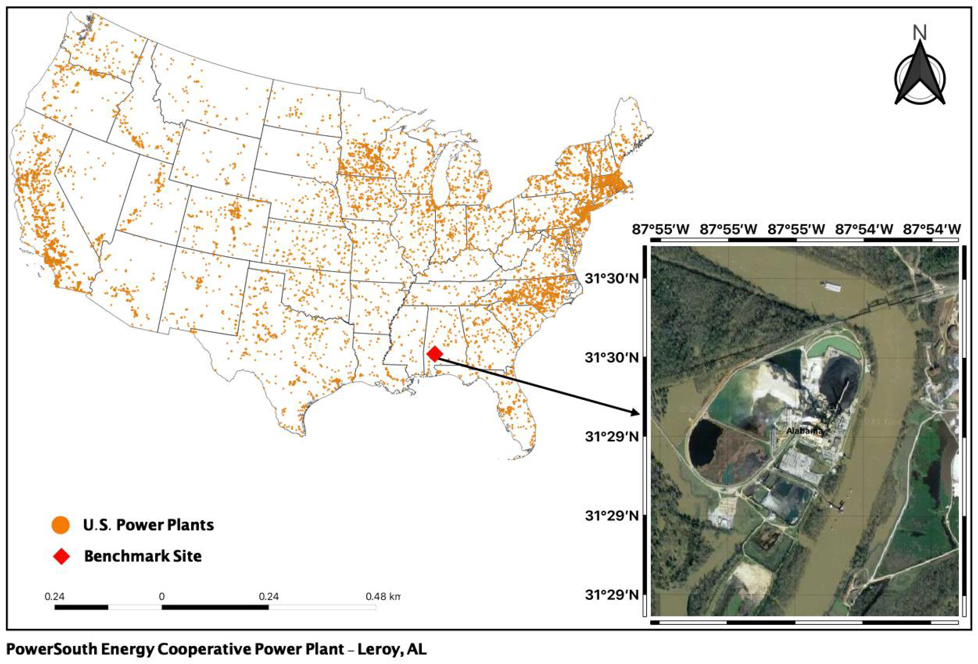
Our general study region covers coal-fired power plants in the United States, with two testing scenarios set up for this study. As our benchmark site, we used a single power plant (first scenario) in rural Alabama (Figure 1). It is about 66 miles south of Mobile, AL. The plant was chosen as it is far away from cities and other emission sources that could introduce noise to the remote sensing observations. Additionally, studying isolated power plants gives us a clear idea of the impact to the population or natural environments.
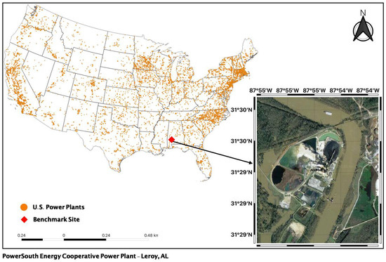
Figure 1.
Location of benchmark site and all U.S power plants (Satellite Image Courtesy: Google Earth. 3 December 2021).
The second scenario set of experiments focused on combining all coal-fired power plants throughout the U.S. This was set as a goal to study the performance of machine learning models in this context and their ability to generalize prediction accuracy for NO2. Obtaining a large-scale emissions prediction for all the power plants gives an additional perspective on the impact of pollutant emissions on the climate. A machine learning model that predicts regardless of location is as beneficial as location-based predictions.
3.2. Data
3.2.1. TROPOMI Tropospheric NO2 Data
The TROPOspheric Monitoring Instrument (TROPOMI) onboard the Sentinel-5 Precursor (S5P) satellite launched on 13 October 2017, and its operational data collection started in April 2018. TROPOMI provided a daily high resolution of 7 × 3.5 km before August 2019 and a higher resolution of 3.5 × 5.5 km after that. One of its L2 products is a tropospheric vertical column of NO2 per mol/m². TROPOMI NO2 data was extracted from Google Earth Engine. To ensure image clarity and accurate emission reflection, TROPOMI only samples during the day in the presence of sunlight. TROPOMI passes over and samples a given location based on its latitudinal distance from the equator, with the local equator crossing time being 13:30 h.
Additionally, TROPOMI provides quality control through its “qa_value” flag for each ground pixel to indicate the quality of the retrieved pixel. The quality per pixel ranges from 0 (no output) to 1 (clear) (Wang et al. [28], 2020). The “qa_value” in the data collected for this study included pixel quality over 0.75 for the tropospheric vertical column of NO2. As a result of this quality control, some days of the year were left out of our dataset, resulting in gaps.
Validation of TROPOMI values against ground-based observations is a widely discussed aspect of TROPOMI. Several studies have measured and attempted to validate the tropospheric data from the S5P satellite, with many discussing the differences observed compared to ground-based measurements. (Verhoelst et al. [27], 2021). A similar monitoring instrument to TROPOMI is OMI (Ozone Monitoring Instrument). It was considered, but due to its lower resolution of (13 km × 25 km) [29], its benefit seemed unlikely and has not been included in this study. TROPOMI NO2 was used as input in our experiments; to mitigate the ML models relying on only one remote sensed data for NO2 prediction, additional data sources were collected.
3.2.2. MERRA-2 Meteorology Data
The second Modern-Era Retrospective Analysis for Research and Applications, Version 2 (MERRA-2), was utilized for its monthly/weekly/daily mean data collection. These collections include assimilations of single-level meteorological diagnostic data, such as temperature at 2 and 10 meters, wind components at 2, 10, and 50 meters, surface pressure, and total precipitable water. This is coarser data, so only one grid point was used for each power plant. This data was utilized as input for the study’s first scenario experiments to test if meteorological features influenced the performance of the ML models.
MERRA-2 has several different types of data that were used, specifically surface temperature, bias-corrected precipitation, cloud fraction, and surface wind speed. The data collected from MERRA-2 were provided on a horizontal grid. The grid has 576 points in the longitudinal direction and 361 points in the latitudinal direction corresponding to a resolution of 0.625° × 0.5°. MERRA-2 validation was compared to ground measurements; strong correlation and low errors were found for air temperatures with a 0.99 correlation coefficient observed and 0.81 and 0.99 for wind speed (Khatibi et al. [30], 2021).
3.2.3. EPA eGRID Data
Emission and Generation Resource Integrated Database (eGRID) data from the Environmental Protection Agency (EPA) was used to validate the training data. This data provides an inventory of environmental attributes of power plants in the United States by tracking air pollutants, such as SO2, CO2, and NO2 per lb/MWh.
The continuous emission monitoring system (CEMS) validates the data collected using the procedure, “Quality assurance requirements for gas continuous emission monitoring systems used for compliance determination”. This procedure is primarily concerned with determining compliance by evaluating the efficacy of quality control (QC) and quality assurance (QA) of data provided by any operational CEMS. It specifies the minimal quality assurance requirements for controlling and quality of any CEMS data provided to the Environmental Protection Agency (EPA) [31]. Any owner of a CEMS must meet these minimal conditions to submit the data they obtained to ensure its validity.
Additionally, the collected in situ EPA NO2 data for this study came with uncertainty about the accuracy and under-sampling of the estimates. EPA releases a “National Emissions Inventory” (NEI) every three years as an estimate of emissions of criteria pollutants [32]. This study utilized remotely sensed data as a representation of in situ data. EPA NO2 was used as the target variable to predict for this study.
3.2.4. U.S. Power Plants Data
Power plant metadata and location shapefiles were obtained from the Energy Information Administration (EIA). The shapefile was dated January 2020 and included 9768 power plants, 289 of which were coal-fired. “Plant Code”, “Plant Name”, “Utility Name” and “Utility ID”, “Sector Name”, “Address”, “Primary Source” (e.g., coal, solar, etc.), power plant capacity per MW (megawatt), and the plants’ latitudes and longitudes were among the features included for each power plant.
3.2.5. MODIS MCD19A2
MCD19A2 is a Level 2 product of aerosol optical depth (AOD) which is calculated by combining terra and aqua imagery into one single multi-angle implementation of atmospheric correction (MAIAC) model. It is produced daily at 1 (km) resolution, and this study used the blue band AOD at 0.47 µm Science Dataset (SDS) layer. The “QA” bands contain flag information about cloud, adjacency, surface type, and surface change. In this study, we collected data that had a cloud-free QA band. This dataset’s inclusion was motivated by the effects of aerosol optical depth on pollutant dispersion, tropospheric NO2 retrieval, and correlation to meteorological conditions (El Khoury et al. [23], 2019; Lin et al. [24], 2019). MCD19A2 was used as input in this study.
3.3. Preprocessing & Post-Processing
3.3.1. eGRID Data Preparation
EPA NO2 data was collected in an hourly format for the whole year and averaged by day. In order to scale the data, it was divided by 1 × 10⁵ and rounded to five decimals. The scale applied to this feature is indicated by the dataset label “EPA NO2/100000”. This feature was then merged with the other data sources listed below for each day of 2019. The number of EPA NO2 values merged in the dataset for a power plant location was determined by our TROPOMI NO2 available data. Certain power plants in the dataset had less than a full year of data due to TROPOMI NO2 QA filtering, resulting in gaps.
3.3.2. TROPOMI Data Preparation
To achieve a precise observation of power plant NO2 emissions observed in TROPOMI images, preprocessing considered the emission and wind movement speeds present in the imagery. Clipping the images based on the latitude and longitude of each power plant was applied, with the breeze wind speed (10–20 mph) and emission traveling speed (assumed 240–480 miles per day) as clipping bounds. If this was not done, the density of the emissions across the images would gradually disperse and become lower with longer distances. In order to obtain an accurate representation of TROPOMI NO2 for each power plant, the spatial scope was essentially shrunk by 7 miles (0.1 degrees) as the height and width of the bounding box to be utilized for clipping. This created a bounding box containing the most affected region in each image while also reducing nearby power plants’ impact (noise).
TROPOMI NO2 value was then extracted from the raster matrix and written to a CSV file - after rescaling the value by multiplying it by 1000 and labeling the feature “TROPOMI*1000” to be on the same scale as EPA NO2 feature-along with the power plant ID, coordinates, EPA NO2 (eGRID), and MERRA-2 data.
3.3.3. MCD19A2 Data Preparation
The Moderate Resolution Imaging Spectroradiometer (MODIS) Land Aerosol Optical Depth (AOD) product is produced daily with hourly values at a 1 km pixel resolution to be utilized in this study, with its blue band (0.47 m) aerosol optical depth over the land product collected for our first scenario power plant. Google Earth Engine was used to obtain the power plants hourly MCD19A2 values in 2019. The image collection “MODIS/006/MCD19A2_GRANULES” was selected and filtered by date starting from 1 January 2019 to 1 January 2020. A filter bound was then applied, based on the coordinate, and the image collections “Optical Depth 047” band was selected.
The extracted image was fed into a reducer, which produced an hourly value after computing the (weighted) arithmetic mean over the area of each band selected for the image. This generated a CSV file with a timestamp and an hourly value for “Optical Depth 047”, which was then resampled to produce a daily average output for the entire year. The inclusion of this data source was an attempt to verify if any improvement could be applied to the machine learning models discussed in this paper.
3.3.4. TROPOMI/EPA Value Pairs
This section discusses combining TROPOMI and EPA data as value pairs associated with each power plant by each daily emission product for each day of the year. Iterating through each power plant in our dataset, an EPA NO2 value was associated, based on the selected facility id and coordinates passed to the EPA (eGRID) dataset. If data existed for the plant and was not empty, a TROPOMI NO2 value was associated with the pair by passing the coordinates of the power plant to TROPOMI images for clipping to obtain their values extracted from the raster object.
Representing the data by pairs of our most impactful features simplified the reshaping and scaling performed in preprocessing before the ML models were fed the data. Obtaining TROPOMI values of the power plant image, the corresponding EPA data for the power plant, monthly averaged MERRA-2 features, and the date string before separation, a CSV file was generated that contained the six features.
3.3.5. Dataset Preparation
Scaling was the first step taken with the data across all ML models in both scenarios. All features in the input variables were scaled on a (0, 1) scale for consistency and performance of the ML models. The scaling prevents giving more weight to higher-range features while less to lower-range features. Both the independent and dependent features were scaled. The predictors and target features for both the train and test sets were then extracted using a 66% training split. Additionally, a datetime string was associated with the CSV file for each day available in the dataset throughout the year. This was split into three separate columns as the ML models cannot parse date strings as input. We transformed the date column numerically into “dayofweek”, “dayofmonth”, and “dayofyear”.
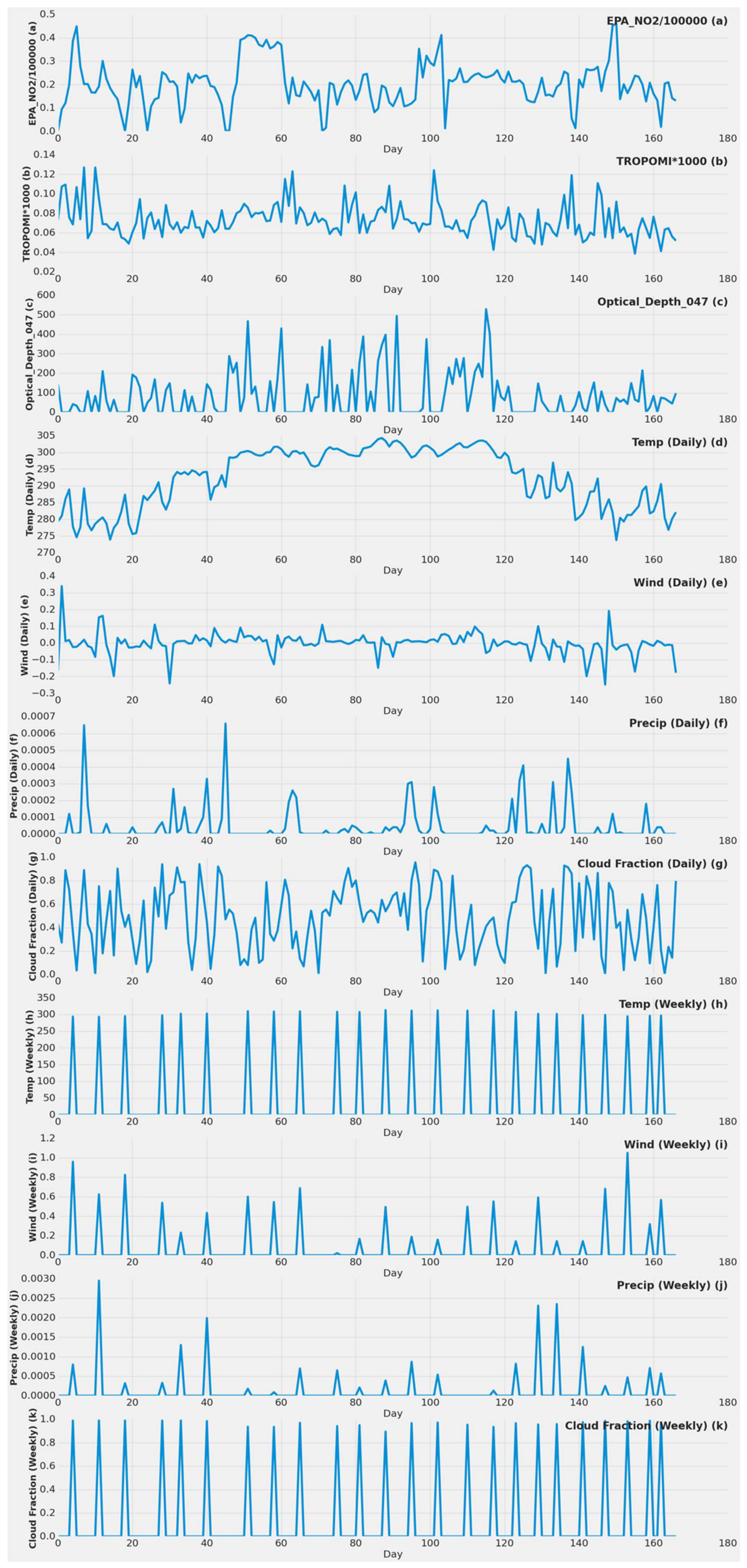
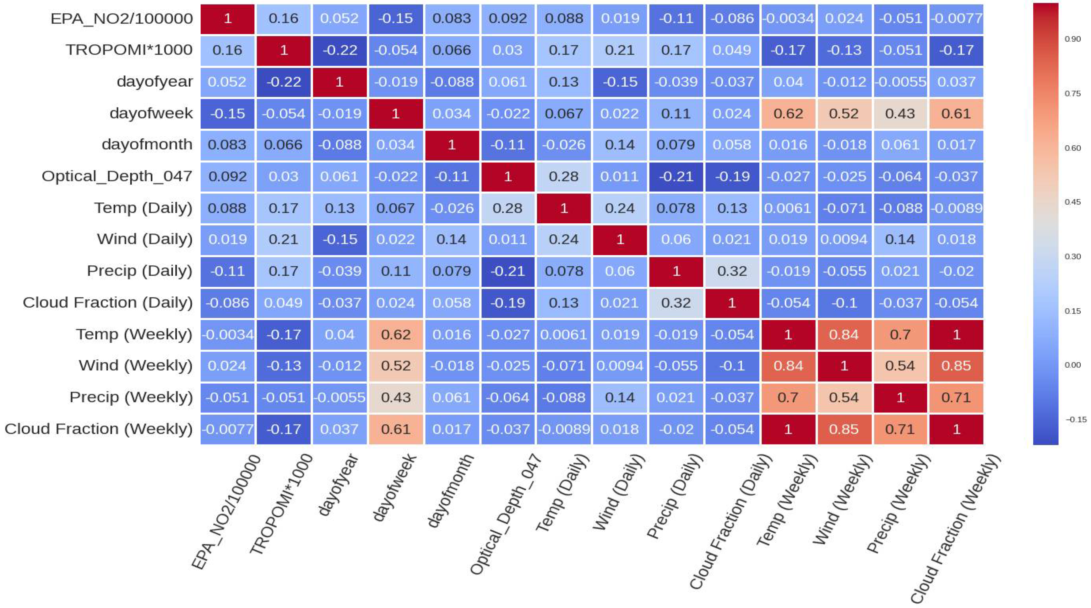
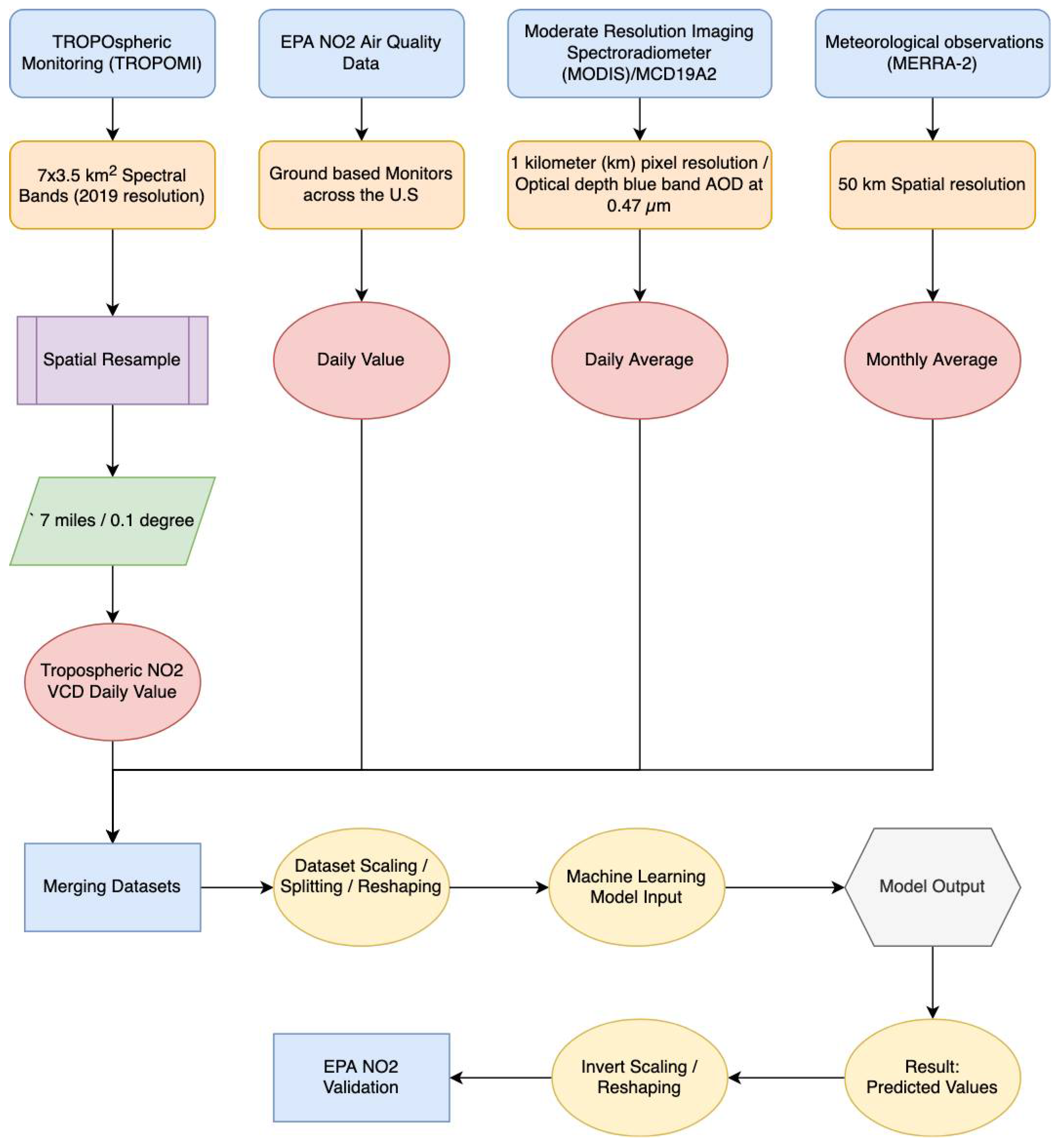
The second scenario included an additional step in which all power plant NO2 emissions were averaged by date. The models would not learn since the dates in a dataset containing all power plants would always overlap. The best approximation of NO2 emissions from all plants was produced by grouping the dataset by date. Because grouping by facility ID removes the dataset’s time series element, resulting in an inaccurate portrayal of emissions over time, it was not used. The final output of both scenarios’ datasets is displayed in Table 1 and Table 2. Figure 2, Figure 3 and Figure 4 visualize the data for the first scenario. Figure 2 shows the data over time, and Figure 3 visualizes the distribution of each feature. Figure 4 visualizes the correlation between each feature of the dataset. Figure 5 displays the overall flow of data and ML for the study.

Table 1.
Statistical description for the single power plant (Alabama) dataset with the date column split into three.

Table 2.
Statistical description for the All 289 coal-fired power plants scenario dataset excluding MERRA-2.
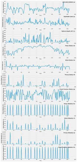
Figure 2.
Actual values throughout the year of different important features for the single power plant (Alabama) dataset. (a) EPA NO2 value by day in 2019; (b) TROPOMI NO2 value by day in 2019; (c) MODIS MCD19A2 blue band AOD at 0.47 µm 2019 value by day in 2019; (d) MERRA-2 daily surface temperature value by day in 2019; (e) MERRA-2 daily surface wind speed value by day in 2019; (f) MERRA-2 daily bias-corrected precipitation value by day in 2019; (g) MERRA-2 daily cloud fraction value by day in 2019; (h) MERRA-2 weekly surface temperature value by day in 2019; (i) MERRA-2 weekly surface wind speed value by day in 2019; (j) MERRA-2 weekly bias-corrected precipitation value by day in 2019; (k) MERRA-2 weekly cloud fraction value by day in 2019.
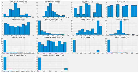
Figure 3.
Distributions of each feature used for training with 10 bins for the single power plant (Alabama) dataset. (a) EPA NO2 distribution in 2019; (b) TROPOMI NO2 distribution in 2019; (c) Number of day distribution in year 2019; (d) Number of week distribution in 2019; (e) Number of month distribution in 2019; (f) MODIS MCD19A2 blue band AOD at 0.47 µm 2019 distribution; (g) MERRA-2 daily surface temperature distribution in 2019; (h) MERRA-2 daily surface wind speed distribution in 2019; (i) MERRA-2 daily bias-corrected precipitation distribution in 2019; (j) MERRA-2 daily cloud fraction distribution in 2019; (k) MERRA-2 weekly surface temperature distribution in 2019; (l) MERRA-2 weekly surface wind speed distribution in 2019; (m) MERRA-2 weekly bias-corrected precipitation distribution in 2019; (n) MERRA-2 weekly cloud fraction distribution in 2019.

Figure 4.
Correlation plot showing the relationship between each feature for the single power plant (Alabama) dataset.

Figure 5.
Data and ML flow.
In some cases (e.g., the LSTM model), additional steps were taken relevant to the model setup. These are discussed in further detail in each model’s section.
3.4. Machine Learning Models
3.4.1. Long Short-Term Memory (LSTM)
This section introduces an LSTM model used for this study. This was chosen as the first model based on one conclusion reached. EPA NO2 target value affected subsequent values in the dataset due to the chronological nature of our data and the long-term effects of pollutants in the atmosphere. The conclusion that a current EPA NO2 value for a day is affected by the previous day’s NO2 value, and an LSTM models’ ability for insensitivity to gap duration in data with some missing days made this choice beneficial. LSTM traditionally is good with non-linear time-series data and can incorporate previous data by time steps, which fitted our data requirement. Three sets of input data were prepared:
- The first set only contained two features (EPA NO2, TROPOMI).
- The second input dataset included MERRA-2 (daily, weekly, monthly), TROPOMI NO2, and date features (EPA_NO2_10000, TROPOMI*1000, dayOfYear, dayOfWeek, dayOfMonth, MERRA-2 Wind, MERRA-2 Temp, MERRA-2 Precip, MERRA-2 Cloud Fraction).
- The third input set contained previously mentioned features and MCD19A2.
The data was then reshaped to a 3-dimensional shape (adding a time axis) required by an LSTM model (number of samples, time steps, number of features). Reshaping must set a look back value specifying how many earlier days are used to create the time series. The input data has X predictors representing feature values at a given time (t) and Y (EPA NO2) representing the value of the next day (t + 1). The time step is measured in days and is set to one, whereas the “look back” value is one week (each time step looks at 7 values). The data was then split into training and testing, with a 66% training split. After scaling, reshaping, and splitting, an LSTM model architecture was built:
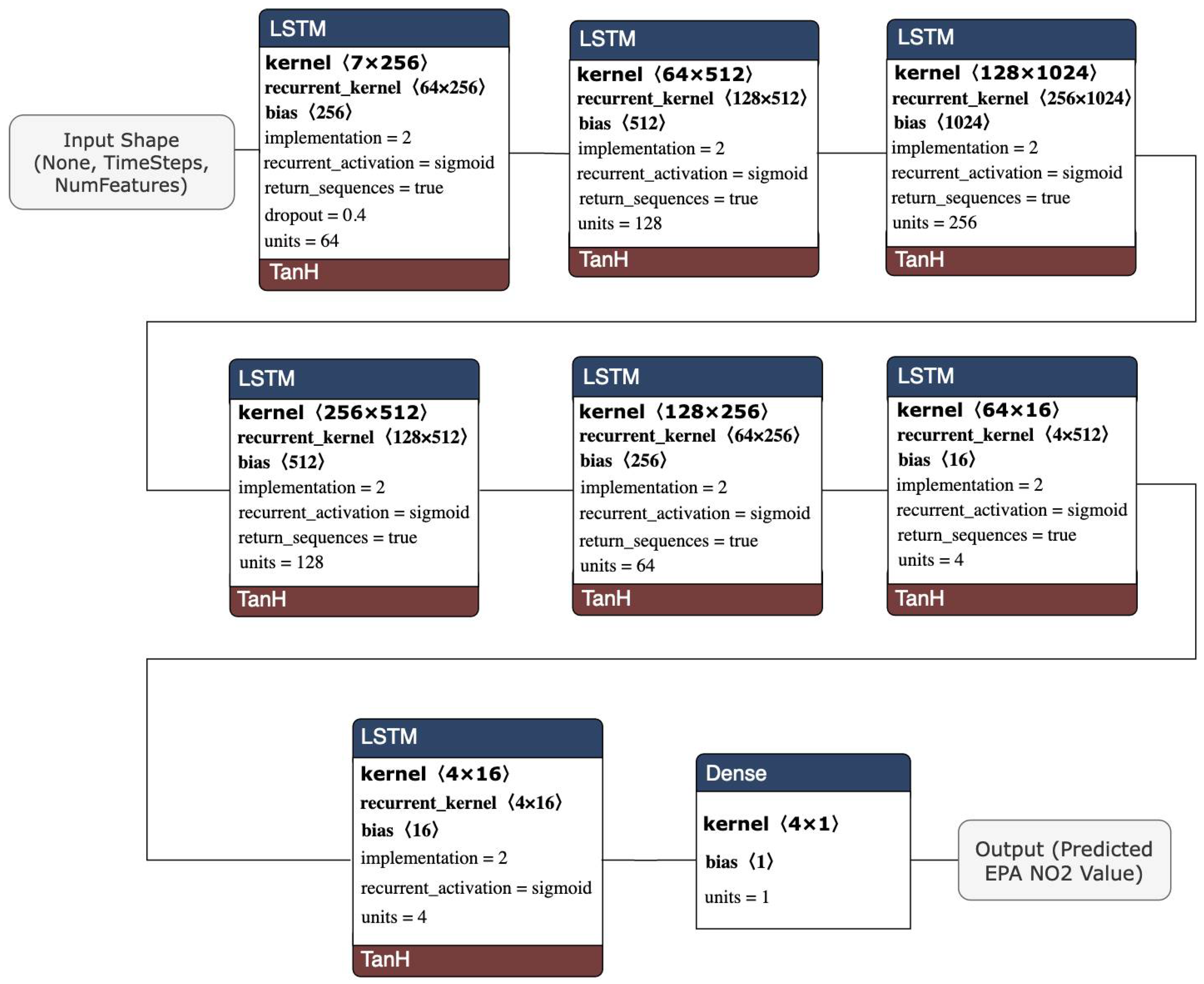
The stacked LSTM architecture model comprised seven LSTM layers, each with (64, 128, 256, 128, 64, 4, 2) units and a dense layer with a single unit. Figure 6 visualizes the architecture of the stacked LSTM model.
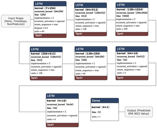
Figure 6.
Stacked LSTM model architecture.
The stacked LSTM model was constructed to be a deeper network topology. The ability for the model to extract and recombine higher-order features embedded in the data for performance improvement was one of the advantages of building a deeper network-especially for a stacked architecture. Each layer of the model passed a recurrent sequence to the next layer to account for the previous time step and to more accurately describe the complex pattern in the nonlinear data at every layer. The model used a dropout setting of 0.4 to reduce overfitting. An MSE loss function was utilized, along with an “adam” optimizer, since it is a typical optimizer in LSTM models and outperformed “rmsprop” in testing. A validation set was provided at training to track accuracy and loss to fine-tune the model. This validation set was not utilized for training but rather to measure the effectiveness of the hyperparameters provided during training.
3.4.2. Support Vector Regression (SVR)
SVR is reliable with non-linear data. As the study’s data was non-linear, an SVR model was used to evaluate the performance capabilities of predicting EPA NO2 emissions and to compare it to the performance of other models in this study.
A radial basis kernel function was selected for this model. The RBF kernel is typically used to find a non-linear classifier or regression line and function for two points X1 and X2 that computes the similarity or how close they are to each other. Separate models were created for each scenario. Each utilized a grid search for a range of values to optimize hyperparameters for each experiment’s scenarios and set of features.
3.4.3. Random Forest
Like the other mentioned models, random forest models can handle nonlinear data and be utilized in regression tasks. Using random forest to build large numbers of decision trees to solve a regression problem was a fit for our use case and prediction problem.
Compared to a decision tree model, the ability of random forest to merge multiple decision trees produces a more accurate prediction. Because random forest is a bootstrap resampling technique that works best with higher dimensions and volume, the result was not exceptional with the study’s volume of data. Separate models were created for each scenario. Each utilized a grid search for a range of values to optimize hyperparameters for each experiments’ scenarios and set of features.
3.4.4. XGBoost
This model is known for its high-performance gradient boosting. XGBoost is highly efficient, flexible in general, and similarly to RF, is a decision-tree-based ensemble machine learning model.
Two different XGBoost models were built, one for the first scenario with varying inputs of feature and one for the second scenario. To fit our non-linear data, the study utilized an XGBoost with a regression squared error loss function. Separate models were created for each scenario. Each utilized a grid search for a range of values to optimize hyperparameters for each experiment’s scenarios and set of features. Because of XGBoost’s well-known high-performance gradient boosting, this model line fit was able to capture the data’s extreme values.
3.5. Model Training Error Metrics
Machine learning approximates a function representing the correlation between inputs and output data. This applies to both linear and non-linear data characteristics. In this study, we used various machine learning models to be trained on the non-linear nature of our data and the relationships between the inputs and output. Measuring the accuracy of the model prediction in the case of regression problems with non-linear data involves standard metrics that measure the performance of the ML models.
Mean absolute error measures the errors between paired observations. Although it is the least looked at metric for measurement, it is a good indicator for understanding the error difference between predicted and actual observations. MAE is insensitive to the direction of errors, and lower values are better (See Equation (1)).
where n is the number of items, and ∑ is the summation notation, and |Yi − Xi| are the difference of absolute errors of predicted EPA NO2 minus observed EPA NO2 values.
Mean squared error measures the average square of errors between the estimated (predicted) values and actual values. It is a risk function that corresponds to the expected values of the squared loss. This metric looks at how close the regression line is to actual values, and lower values are better (See Equation (2)).
where n is the number of items, ∑ is the summation notation, Yi is observed EPA NO2 values, and Ŷi is predicted EPA NO2 values. It is one of the primary metrics used for model performance in this study.
Root mean squared error was utilized as an additional metric. It is a measure of the error rate by the square root of MSE. RMSE is also insensitive to the direction of errors, and lower values are better (See Equation (3)).
where Ŷi is the predicted EPA NO2 values, Yi is observed EPA NO2 values, n is number of items, and ∑ is the summation notation.
The residual standard error measures the accuracy of nonlinear regression models. Similar to the standard deviation, it calculates the average distance of the actual values from the regression line. Additionally, RSE is insensitive to the direction of errors. Lower RSE values mean better results. The residual standard error is defined below (See Equation (4)).
where ∑ is the summation notation. Y is the observed EPA NO2 value. Ŷ is the predicted EPA NO2 value. df is the degrees of freedom, calculated as the total number of observations-total number of model parameters.
The error rate was one of the primary metrics used for model performance in this study. This metric calculates the percentage error rate for all average error distances between actual and predicted values (See Equation (5)).
where the percentage error rate is the result by dividing RMSE using Ȳ which is the mean of target actual values for the test dataset. Error rate provides a comprehensive measurement of predictive performance with lower values being better.
3.6. Tools and Hardware
The code for data collection, formatting, processing, and training were all written in Python 3.6 based on pandas, scikit-learn, Keras, TensorFlow, shapefile, and H2O to create ML models, prepare data, and train and test the models.
We used two different computational environments over the project. Initial data collection and processing were conducted on Microsoft Azure. The main experiment was carried out on three Linux servers with 48 cores Intel® Xeon® Silver 4116 CPU, 128 GB memory, and 4 NVIDIA K80 GPUs.
4. Experiments and Results
4.1. Feature Importance Results
The first stage was to understand all the input variables and their impact. Because MCD19A2 and daily and weekly MERRA-2 were not part of the initial testing, TROPOMI NO2, monthly average wind speed, monthly average temperature, monthly averaged precipitation, monthly averaged cloud percentage, day of the year, day of the week, and day of the month were all assessed without it. Their importance is shown in Figure 7. The static features that did not change for one site, such as latitude, longitude, and site ID, reported no significance. The highest impactful features were TROPOMI NO2, day of the year, and the monthly averaged cloud fraction, ordered from high to low importance. Figure 7 was generated without preprocessing, scaling, or reshaping applied to the features.
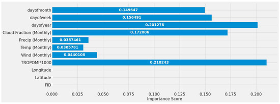
Figure 7.
Early testing random forest models’ feature importance using all features for a single power plant (Alabama) dataset.
4.2. Early Testing
The study undertook preliminary testing to determine whether such predictions could be established for this study. The initial testing experiments involved linear regression, random forest, multilayer perceptron, and voting ensemble. High error rates of around 50% were observed, indicating random predictive capability, but they pointed to areas where preprocessing, feature selection, and model selection may be improved. The second phase of experiments utilized LSTM, support vector regression, random forest, and XGBoost models for their ability to handle non-linear data. This resulted in a lower prediction error rate and increased accuracy.
The early testing experiments were executed without any preprocessing, other than combining the separate datasets and power plant information. As expected, the results were unsatisfactory, highlighting the need for preprocessing techniques, such as feature scaling and train and test splitting.
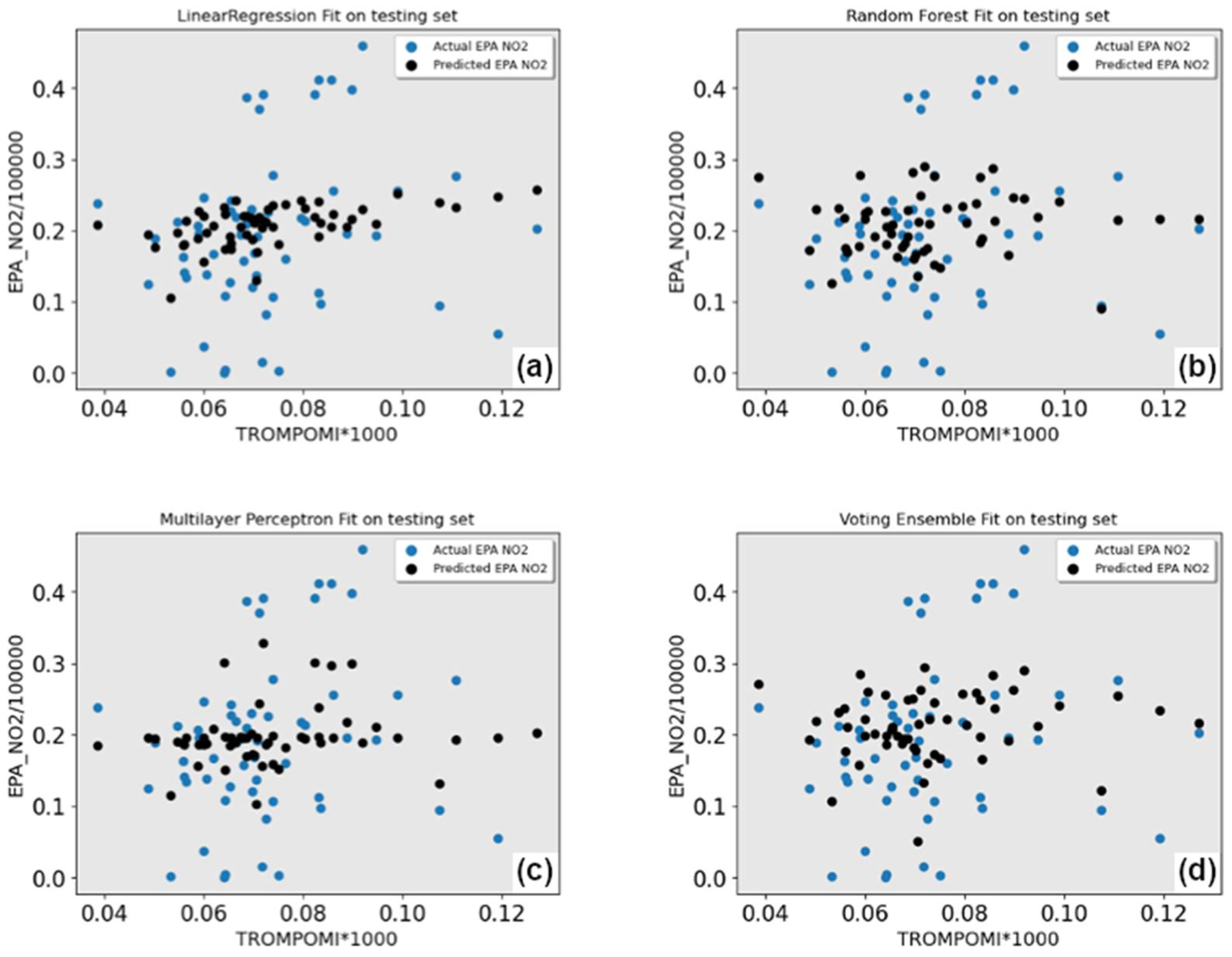
The results of the initial runs are shown in Table 3, and the visual results are shown in Figure 8. Four ML models in Table 3 are presented. Of the four ML models, linear regression had the worst performance, with the mean average error (MAE) and mean square error (MSE) slightly higher than the other models. The other three models produced similar results, with RF having the lowest error rate and residual standard error, making it the best model in this first cycle of the tests.

Table 3.
Results of four ML models executed as initial experiments.
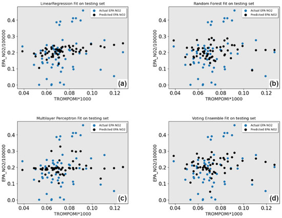
Figure 8.
Early testing experiments. Blue dots are actual, black is predicted. (a) Linear regression model results; (b) Random forest model results; (c) Multilayer perceptron model results; (d) Voting ensemble model results.
4.3. Improved ML Models
4.3.1. LSTM Results
This section introduces the results of the long short-term memory (LSTM) model. We tested performance with many feature set variants for the LSTM models. For all the LSTM experiments listed below, a batch size of 1 with a learning rate of 1 × 10⁻³, no early stopping set, and a dropout setting of 0.4 were used as they were the most optimal values, yielding the results shown in Table 4, Table 5, Table 6 and Table 7. Figure 9, Figure 10 and Figure 11 show the results of the stacked LSTM models at epochs 250, 380, and 430.

Table 4.
Test set validation results of multiple stacked LSTM model experiments for a single power plant (first scenario).

Table 5.
Actual EPA NO2 values from test set compared to predicted values from a stacked LSTM model with 380 epochs using a single plant (Alabama) dataset including MERRA-2.

Table 6.
Test set validation results of multiple stacked LSTM model experiments using all power plant data in 2019 for the second scenario.

Table 7.
Test set validation results of a support vector regression model for the two study scenarios.

Figure 9.
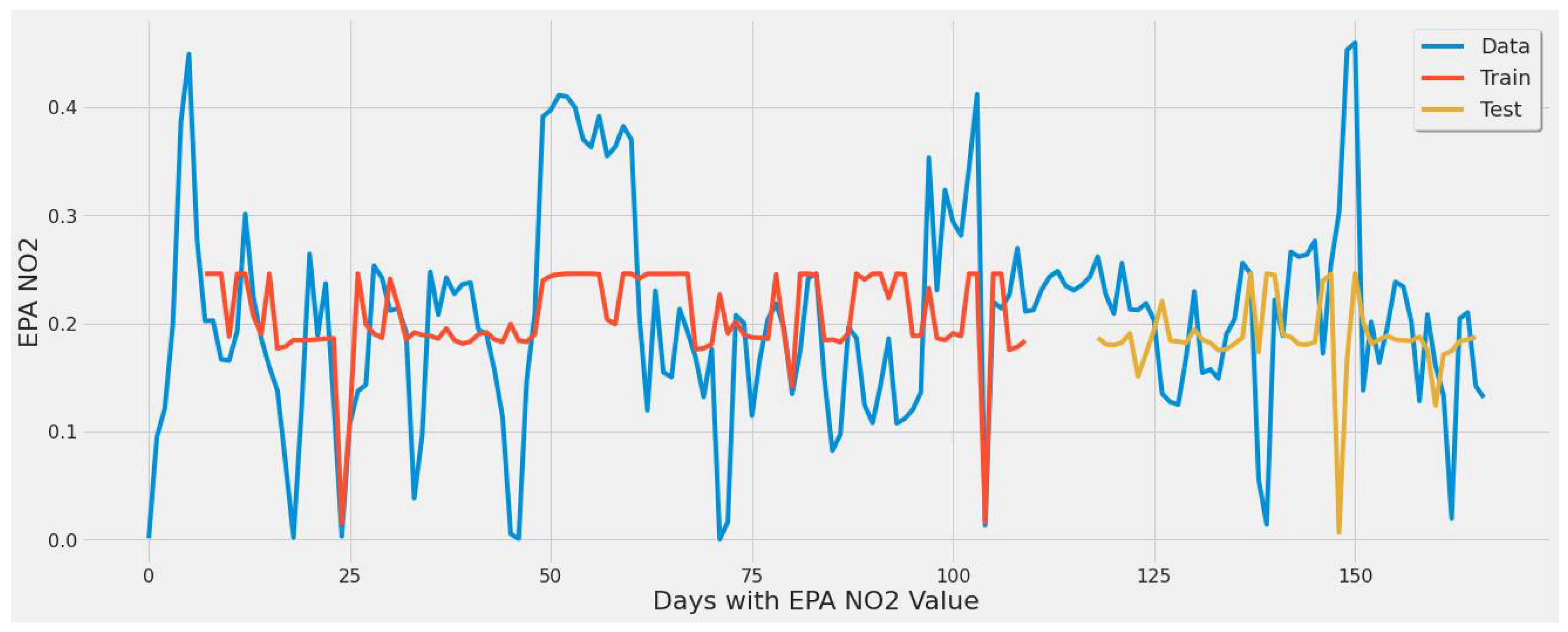
Graph showing the LSTM model [250 epochs] capture of EPA NO2 values over the year using a single plant.
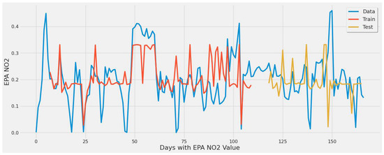
Figure 10.
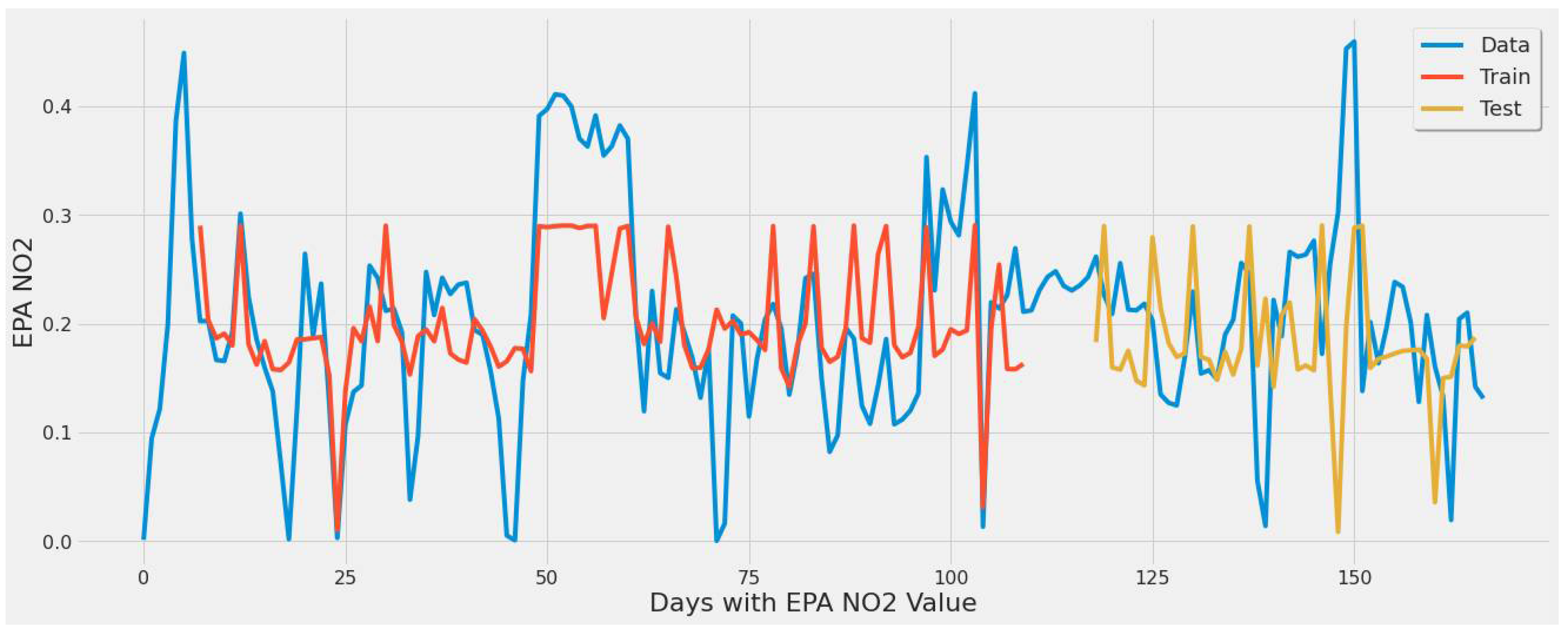
Graph showing the LSTM model [380 epochs] capture of EPA NO2 actual values over the year using a single power plant.

Figure 11.
Graph showing the LSTM model [430 epochs] capture of EPA NO2 values over the year using a single power plant.
Figure 9 largely underestimated EPA NO2. This figure corresponds to LSTM experiment #1 (Table 4). The error rate of 46.85% ranked best for the first three experiments using only TROPOMI NO2 as input and 250 epochs but ranked fifth worst between all experiments and different feature set combinations in Table 4. This was primarily due to the lack of input features used for training. The error rate increased by increasing the epochs to 380 and 430, which was indicative of its inability to further learn any patterns in the EPA NO2 data.
Figure 10 offers a model that is not over or underfitting while capturing some of the actual EPA NO2 data trends (peaks, declines) during the year. This figure corresponds to LSTM experiment #2 (Table 4).
Regarding learning patterns for extreme values found in EPA NO2 data, Figure 10’s stacked LSTM model showed more generalization than Figure 9 and Figure 11 based on the line fit for training and testing sets. The evaluation performed on the train and test datasets in Figure 10 had an error rate of 43.83% for the test set and 39.8% for the training set. These results indicate the model is not overfitting; otherwise, the training error rate would be much lower, and the test set larger.
Figure 11 corresponds to LSTM experiment #3 (Table 4). The error rate increased to 50.4% since the increase in epochs with only one feature (TROPOMI) did not serve as sufficient predictors. Despite having the largest error rate, the MAE was slightly lower than LSTM experiment #2 (most optimal) in Table 4, indicating that individual predictions were closer to actual EPA NO2 on average.
Table 5 lists the actual EPA NO2 values from the test set compared to predicted values for LSTM experiment #5 (Table 4).
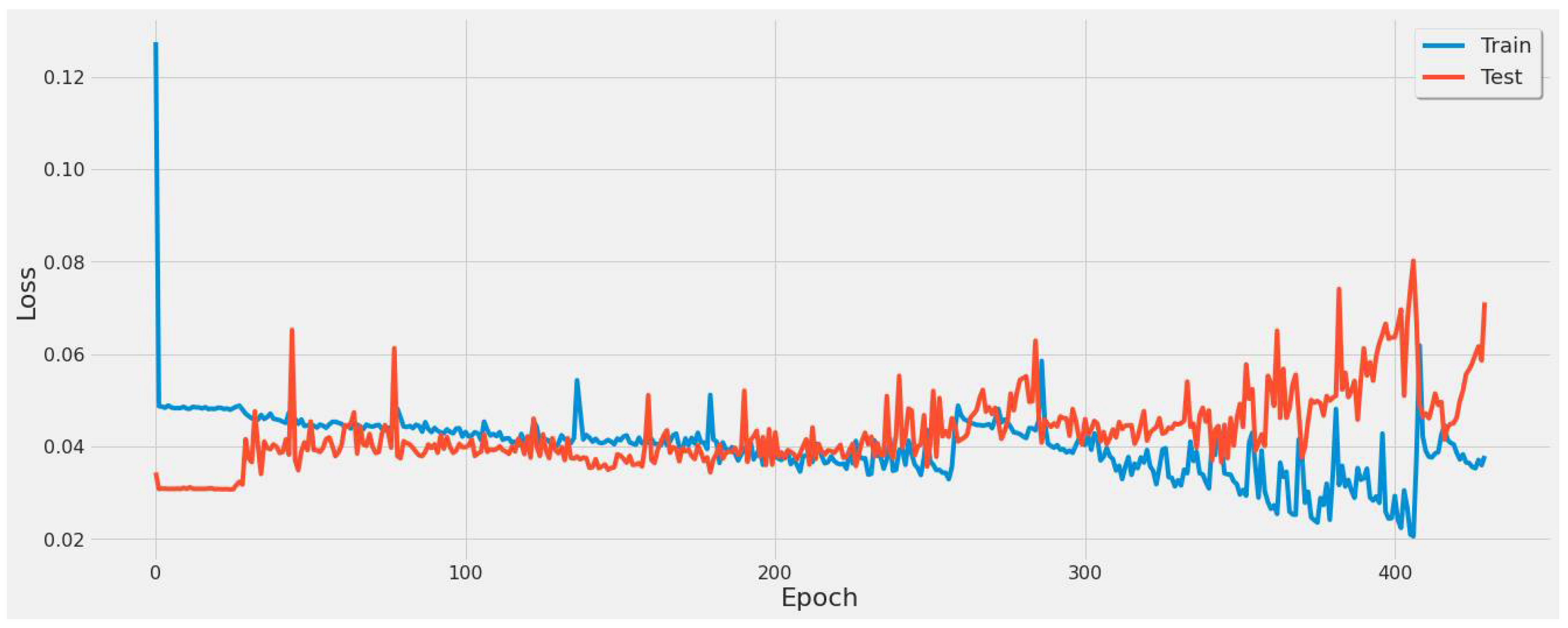
Figure 12 shows the model loss for the 6th experiment with 430 epochs. It revealed certain converging points around 250 and 380 epochs, prompting additional experiments for the various feature sets listed in Table 4 with corresponding epochs. These epoch tests revealed that 380 was optimal across all experiments.

Figure 12.
Graph of model loss through a 430-epoch training cycle for the stacked LSTM model using a single power plant.
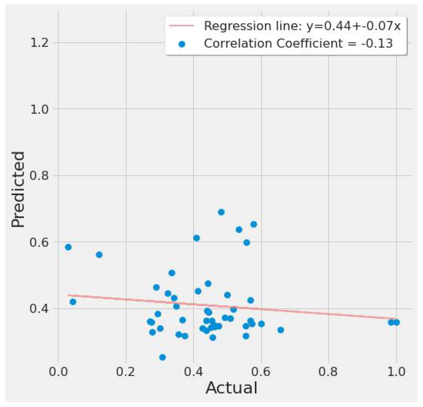
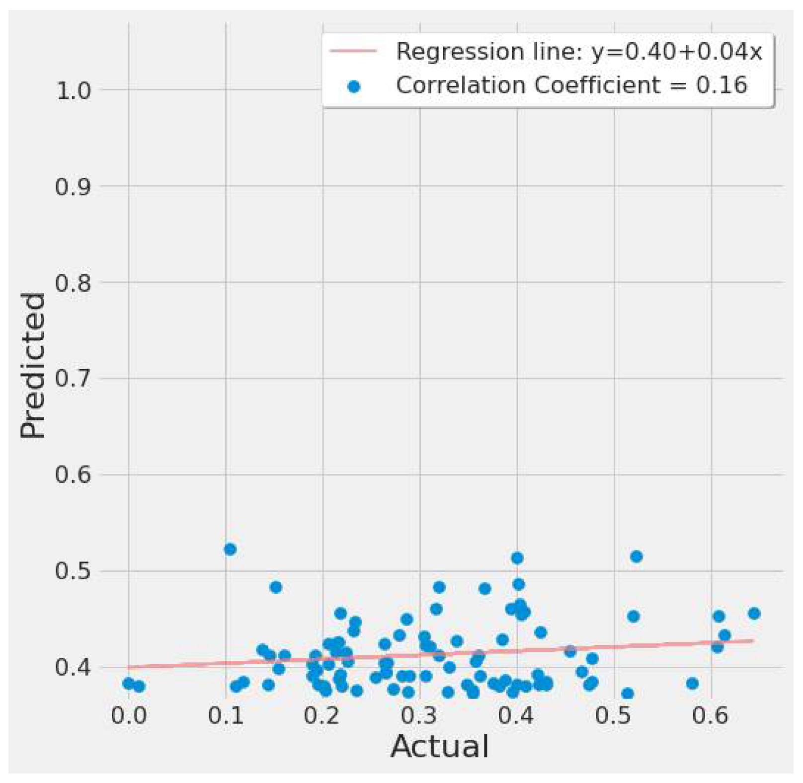
A correlation plot of actual vs. predicted EPA NO2 values is shown in Figure 13 and Figure 14. Figure 13 shows a weak negative correlation for the first study scenario, whereas Figure 14 shows a weak positive correlation for the second scenario. This is due to the LSTM model’s significant error rate in most tests and seeing a plot with any correlation suggests the LSTM model can at least predict, but erroneously. Figure 13 is based on LSTM experiment #5 (Table 4), whereas Figure 14 is based on LSTM experiment #3 (Table 6).
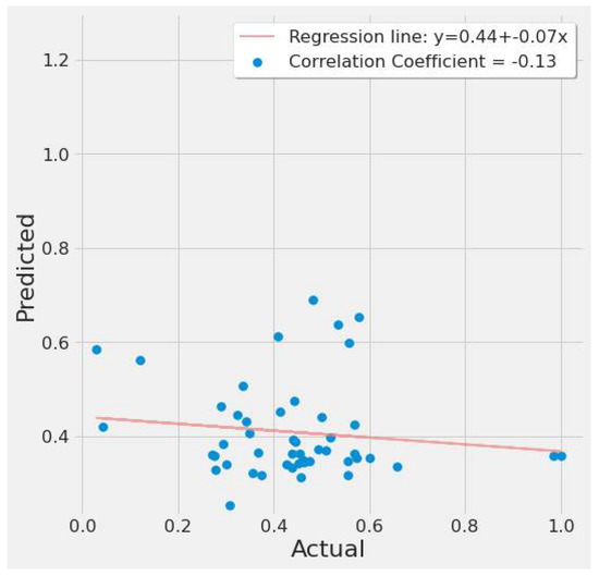
Figure 13.
LSTM actual vs. predicted EPA NO2 correlation plot using TROPOMI and date features for the study’s first scenario.

Figure 14.
LSTM actual vs. predicted EPA NO2 correlation plot using TROPOMI and date features for the study’s second scenario.
LSTM experiment #20 (Table 4) produced the best results in this section based on the error rate for the first scenario. The addition of daily MERRA-2 and MCD19A2, as correlated predictors with the most optimal epoch, reduced the error rate to 39.9% average prediction error. Although this experiment produced the best results, LSTM experiment #10 (Table 4) came in a close second with an error rate of 41.9%. The tenth experiment utilized the same setup as the 20th experiment but without MCD19A2 and TROPOMI, indicating that these datasets only offered a slight performance boost with this model.
The same experiments were applied for the second scenario. Figure 15 corresponds to LSTM experiment #2 (Table 6). It displays the second scenario’s train and test predictions over actual EPA NO2 averaged by date. The experiment had a 63.71 % error rate, which is quite high and indicative of poor predictive ability. Despite the fact that the model in Figure 15 had been tested with various tunings and epochs, the LSTM model failed to predict EPA NO2 in this scenario adequately. Additionally, due to the averaging necessary to avoid EPA NO2 data overlap across date features, this model was biased toward a narrow range of EPA NO2 values between 0.08 and 0.10.
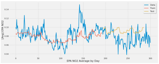
Figure 15.
Graph showing the general model capture [430 epochs] of averaged EPA NO2 values split by train and test sets for all coal-fired power plants second scenario.
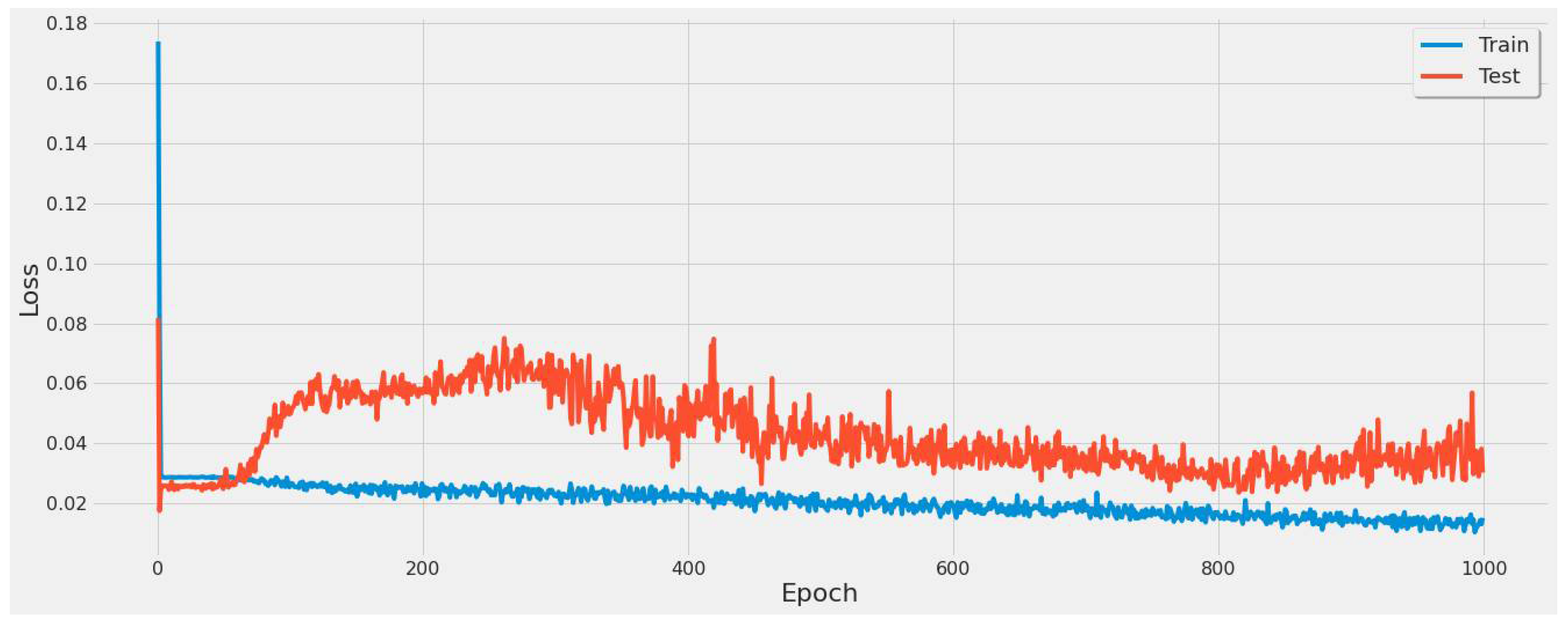
Figure 16 shows the model loss over 1000 epochs. This was conducted to verify if the model had any further convergence points. This figure represents the lack of convergence points and shows that the model achieved the lowest error on a single sample of the data at 800 epochs. This led to an 800 epochs test in Table 6 that yielded the lowest error rate of 55.79% in the second scenario of the experiments.

Figure 16.
Graph of model loss through a 1000 epoch training cycle for the LSTM model all coal-fired power plants second scenario.
4.3.2. SVR Results
This section introduces the results of the support vector regression model. Table 7 shows the performance metrics of experiments. Compared to the early testing results, utilizing an SVR model resulted in a considerable increase in model prediction accuracy. The hyperparameters are included for each experiment in Table 7.
Figure 17 corresponds to SVR experiment #2 (Table 7). Although most extreme values are underestimated, the error rate of 33.6% is a significant improvement over the LSTM model in a similar experiment.

Figure 17.
SVR model fit over actual EPA NO2 actual values throughout the year using a single power plant.
Figure 18 corresponds to SVR experiment #10 (Table 7). This model averaged EPA NO2 across all power plants, introducing bias as most of the averaged EPA NO2 was around 0.08 to 0.10. Still, the model was not overtly overfitting and captured the trend mainly, but the low error rate of 15.52% was influenced by the bias towards the concentrated range of EPA NO2 averaged values.

Figure 18.
SVR model fit over actual EPA NO2 values for training/testing sets throughout the year using TROPOMI/Date features for all coal-fired power plants second scenario.
Figure 19 shows a correlation plot of the predicted vs. actual EPA NO2 for SVR experiment #2 (Table 7). The graph depicts a moderate positive relationship. The regression line is fitted around the cluster of points, indicating a good model fit.

Figure 19.
SVR actual vs. predicted EPA NO2 correlation plot using TROPOMI and date features for the study’s first scenario.
Figure 20 is similar and was generated from SVR experiment #10 (Table 7). It shows a strong positive correlation between actual and predicted EPA NO2 values, with the regression line fitted around the cluster of points.
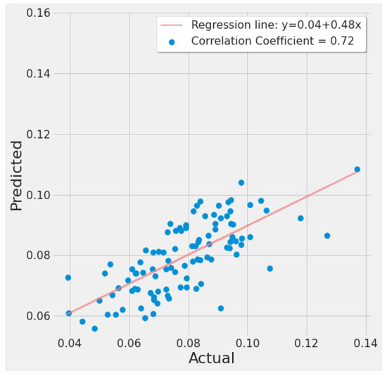
Figure 20.
SVR actual vs. predicted EPA NO2 correlation plot using TROPOMI and date features for the study’s second scenario.
SVR experiment #3 (Table 7) utilized TROPOMI, MERRA-2 daily, and date features. It resulted in the lowest error rate for the study’s first scenario. This experiment resulted in a 13.36% improvement in the error rate in comparison to SVR experiment #1 (Table 7) using TROPOMI NO2 input only. The MAE listed for the third experiment confirm its predictive ability by producing an MAE of 0.0483, indicating a slight difference observed between actual and predicted EPA NO2 values.
The SVR model had the best results across both study scenarios for the lowest error rates of 32.4% (SVR experiment #3) for the first scenario and 15.52% (SVR experiment #10) for the second scenario.
4.3.3. RF Results
The study experimented with random forest for both scenarios and the results are shown in Table 8. The results were comparable to the SVR and XGBoost models while training significantly faster than both. A randomized grid search was used to optimize the hyperparameters for the scenario and set of features used in each experiment. Table 8 lists the settings for different experiments.

Table 8.
Test set validation results of a random forest model for the two study scenarios.
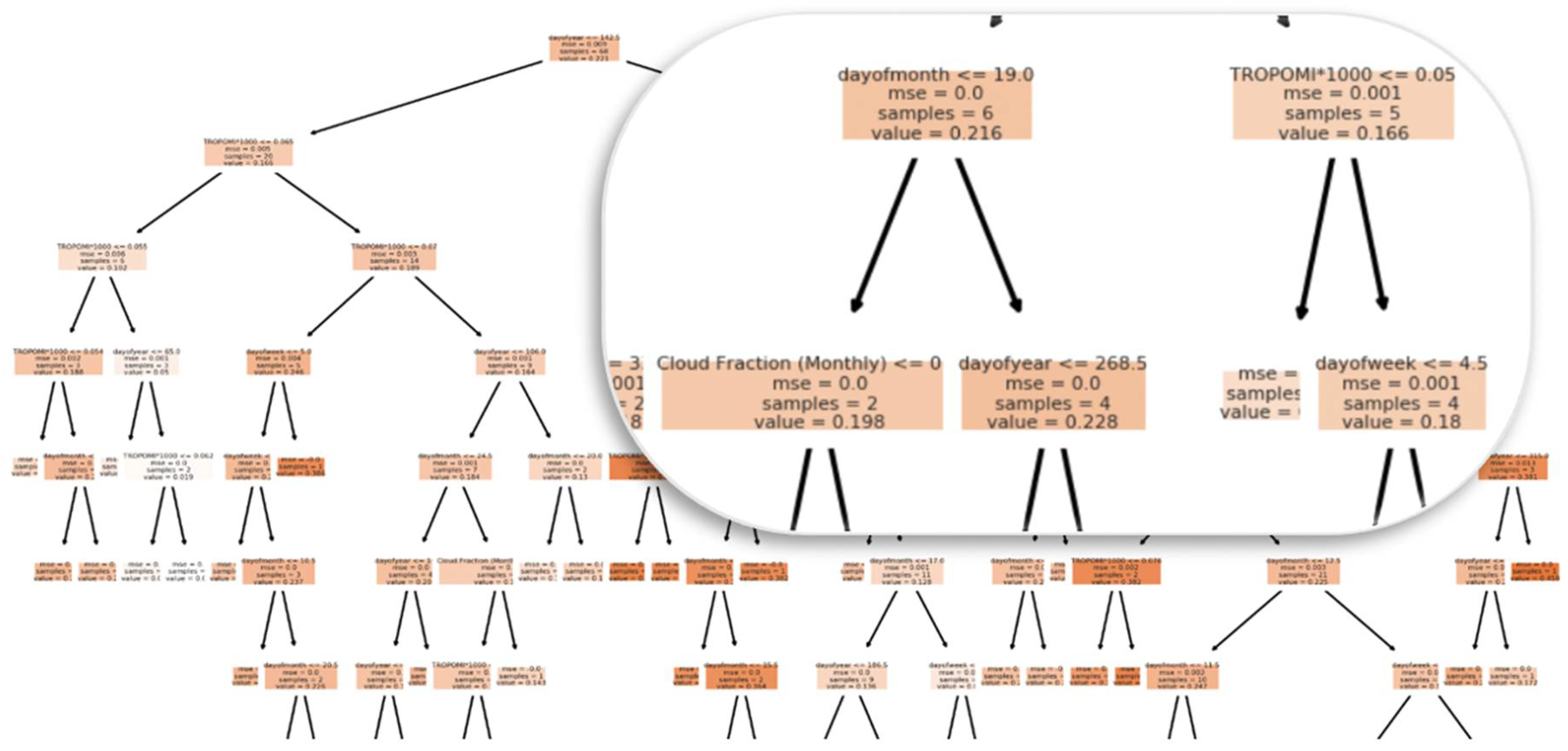
Figure 21 displays the decision tree generated from RF experiment #2 (Table 8). The tree split started with the “dayofyear” feature by taking the middle point value of the year. TROPOMI NO2 and date features split all subsequent nodes. Each split was performed with values higher than a threshold the model set. A sample was taken from the dataset to calculate the MSE of the predicted EPA NO2 error distance from the regression line until a leaf (terminal) node was constructed, determining the optimal EPA NO2 prediction.
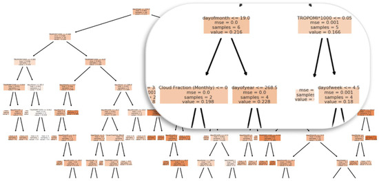
Figure 21.
Graph showing the random forest decision tree nodes and splits.
Figure 22 corresponds to RF experiment #4 (Table 8). The plot mostly shows underestimation for the test set line over actual values. The feature set utilized resulted in performance slightly behind RF experiment #3. The figure showcases the model’s inability to learn the patterns even with different feature sets listed in Table 8.

Figure 22.
Random forest model fit over actual EPA NO2 values for training/testing sets throughout the year using all features of a single power plant (Alabama) dataset.
Figure 23 corresponds to RF experiment #12 (Table 8). The plot graphs the second-best result behind SVR’s similar experimental setup for the study’s second scenario to show a good prediction fit over actual EPA NO2. Specific points in the yellow line pick up some extreme values, while others are estimates.
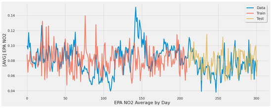
Figure 23.
Random forest model fit over actual EPA NO2 values for training/testing sets throughout the year using all features for all coal-fired power plants second scenario.
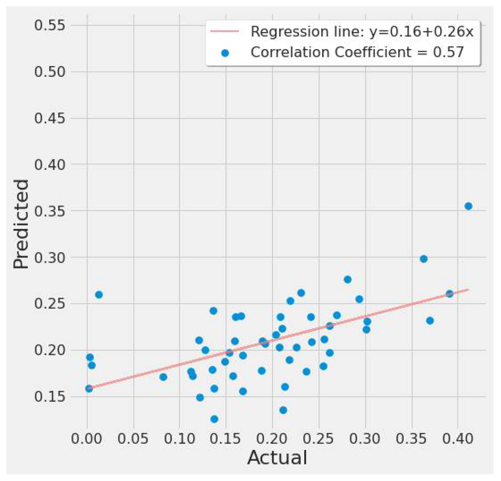
Figure 24 is generated from the results of the RF experiment #4 (Table 8) and depicts a moderate positive relationship. The regression line is fitted around the cluster of points, indicating a good model fit.

Figure 24.
Random forest actual vs. predicted EPA NO2 correlation plot using TROPOMI and date features for the study’s first scenario.
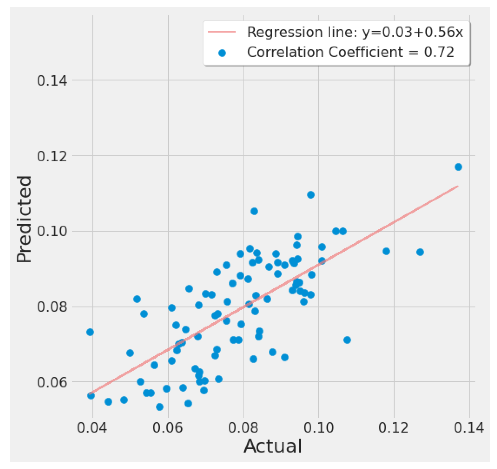
Figure 25 is generated from the last experiment in Table 7 and shows a strong positive correlation between actual and predicted EPA NO2 values indicating a good model fit.
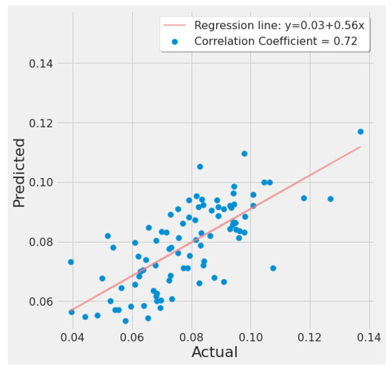
Figure 25.
Random forest actual vs. predicted EPA NO2 correlation plot using TROPOMI and date features for the study’s second scenario.
Figure 26 displays a feature importance graph that the random forest model deemed the most important based on the feature’s correlation score with EPA NO2. It ranked “dayofyear” as the most important due to the trend associated with the time axis and the correlation this feature has with the other input variables. TROPOMI NO2 came second, while another time feature, “dayofmonth” came third. This model determined that MERRA-2 features were not significantly correlated with EPA NO2 and thus has ranked them last.
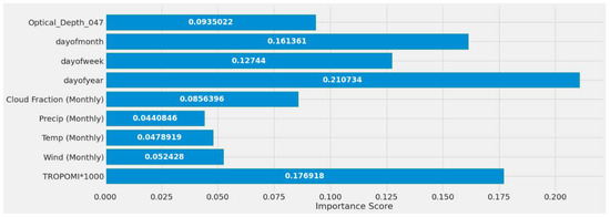
Figure 26.
Random forest models’ feature importance using a single power plant (Alabama) dataset.
Different MERRA-2 temporal datasets were used in Experiments #6 through #10. With daily or weekly MERRA-2 data, this model did not produce greater benefits. The results of the daily MERRA-2 experiments were close to those of the monthly MERRA-2 experiments, however, they were a little behind. This is attributable to the model’s low correlation with the target EPA NO2, which resulted in little performance improvement.
RF experiment #4 (Table 8) lists the error rate of 34.10%, with the MSE being identical to experiment #3 (Table 8) using TROPOMI NO2 feature only. The inclusion of MERRA-2 and date features for this model had little performance boost.
RF experiment #12 (Table 8) produced a low error rate of 15.92% by utilizing a grid search to tune the hyperparameters. Similar to the LSTM model, it is worth noting that this model was somewhat biased toward a narrow range of EPA NO2 values, between 0.08 and 0.10, due to the averaging required to avoid EPA NO2 data overlap across date features.
4.3.4. XGBoost Results
This section introduces the XGBoost model results. Several hyperparameters were set across all experiments listed in Table 9. A maximum depth of 15 to minimize overfitting and 1000 estimators to boost the model’s learning complexity were set. A subsample of 0.7 to sample 70% of the training data before growing additional trees and an “eta” value of 0.1 to minimize the default step size shrinkage and avoid overfitting were used. A repeated K-Fold was used to find the best performance for each experiment. Three folds were provided for the cross validator to resample, each with three repetitions.

Table 9.
Test set validation results of an XGBoost model for the two study scenarios.
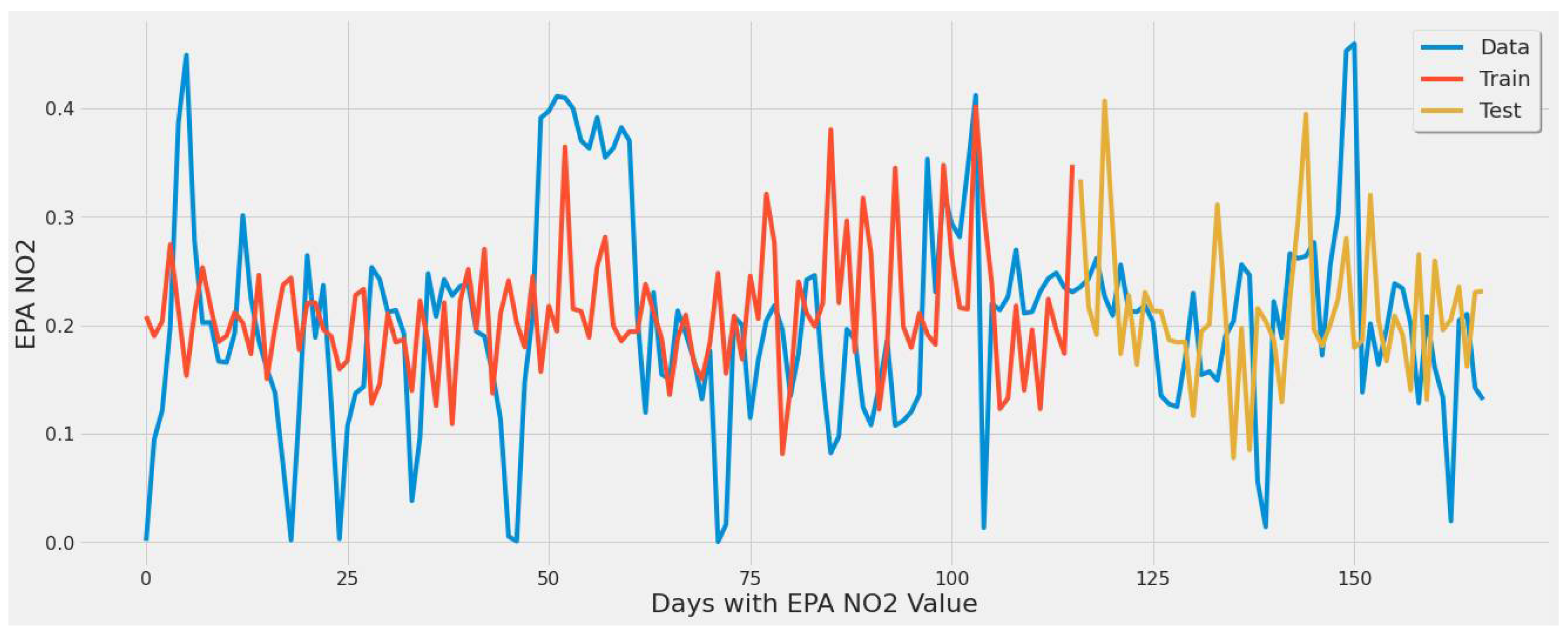
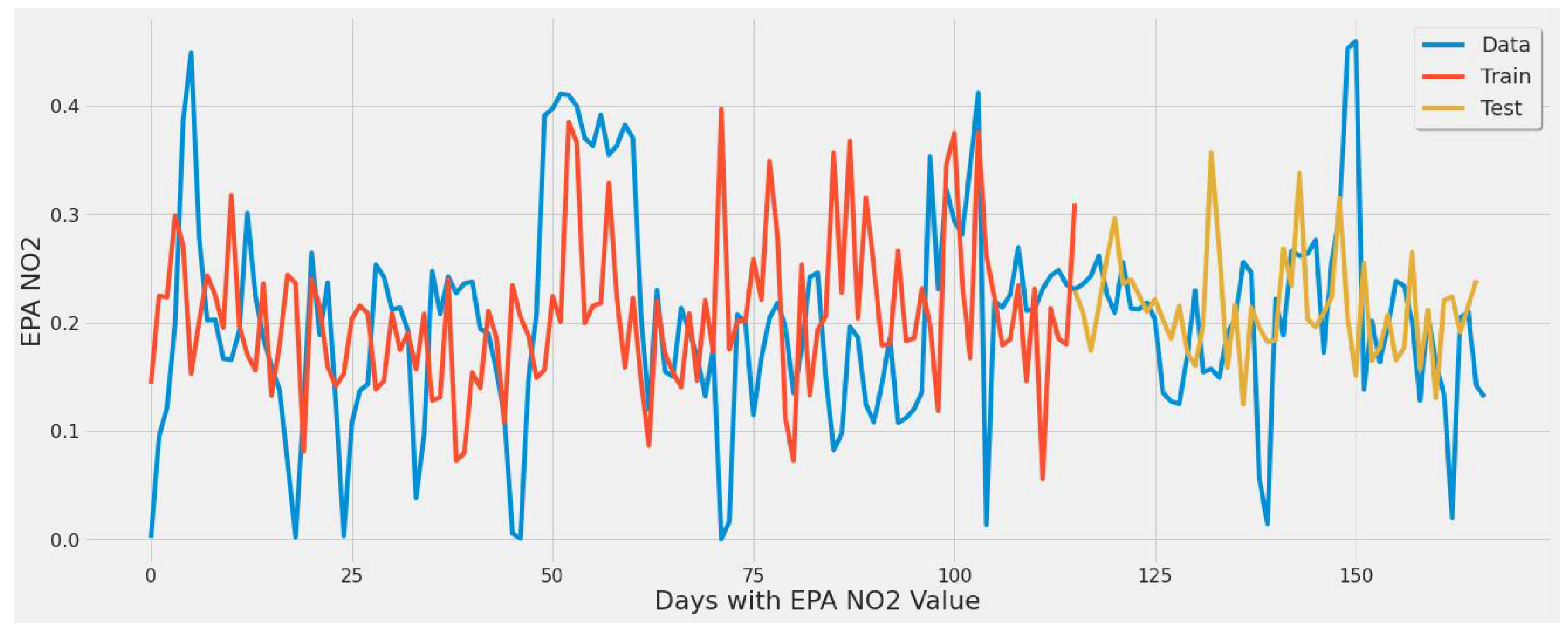
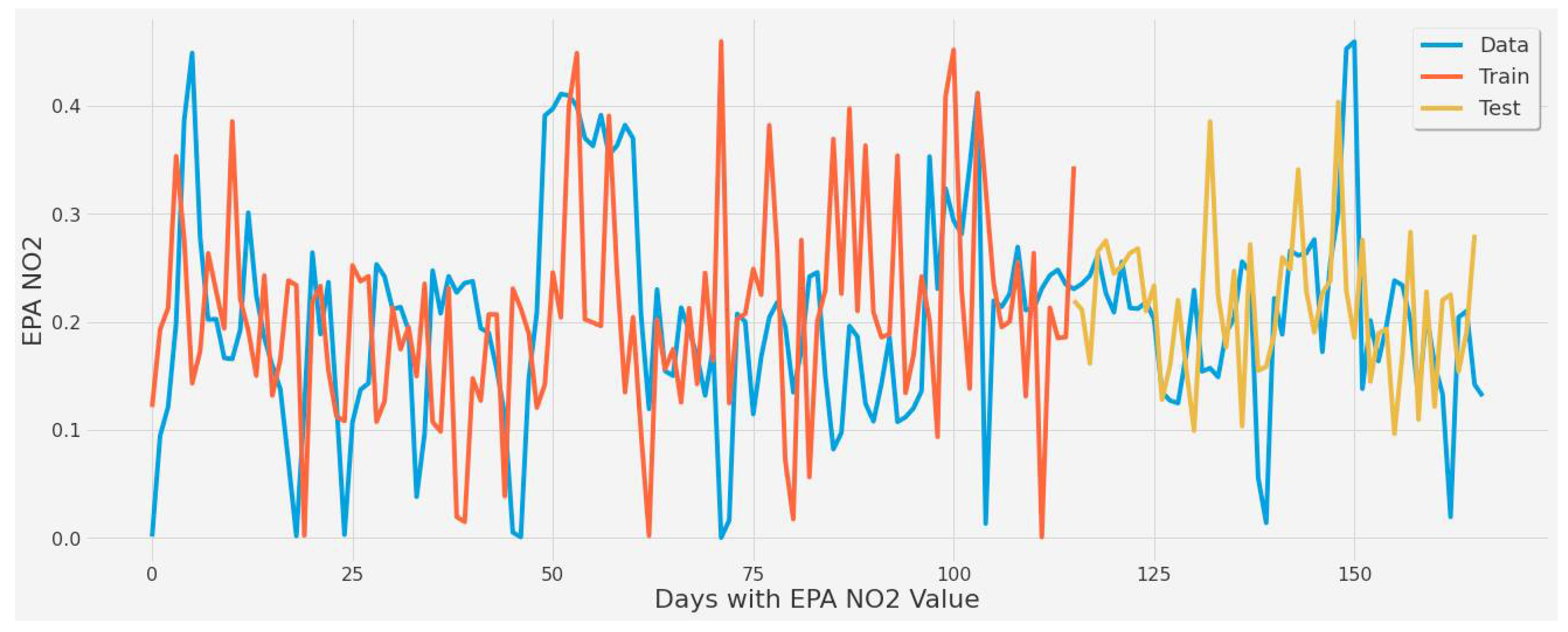
Figure 27 represents XGBoost experiment #2 (Table 9) and shows that the test set was overestimated (yellow line). The model captured some minor peaks and drops rather well (days 125–130) with an error rate comparable to the same feature combination for the RF model and 3% higher than the SVR model. The combination of TROPOMI NO2, MERRA-2 features, and date features resulted in the lowest error rate for this model.

Figure 27.
XGBoost model fit over actual EPA NO2 values for training/testing sets throughout the year using a single power plant (Alabama) dataset.
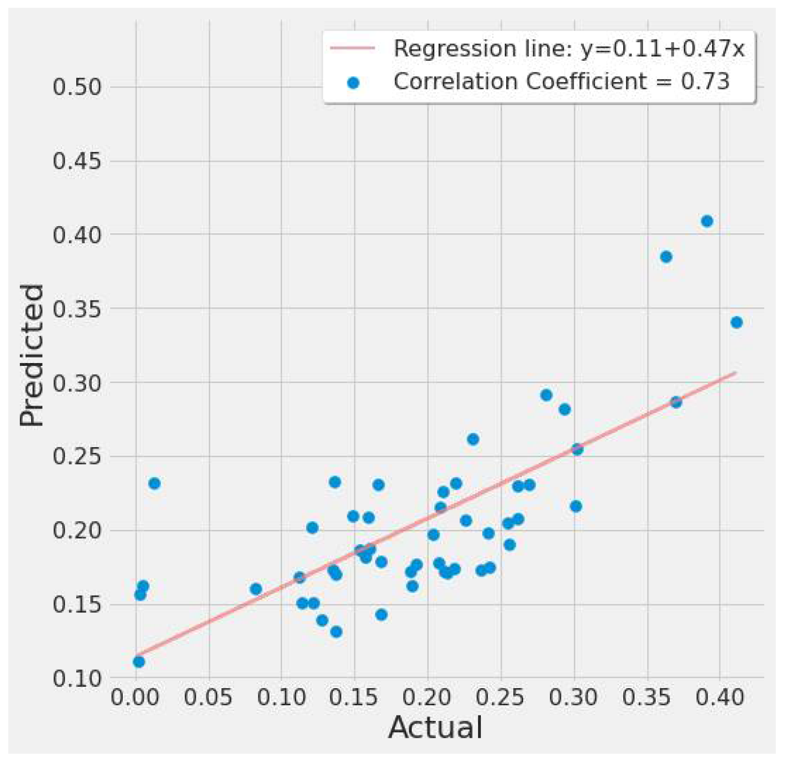
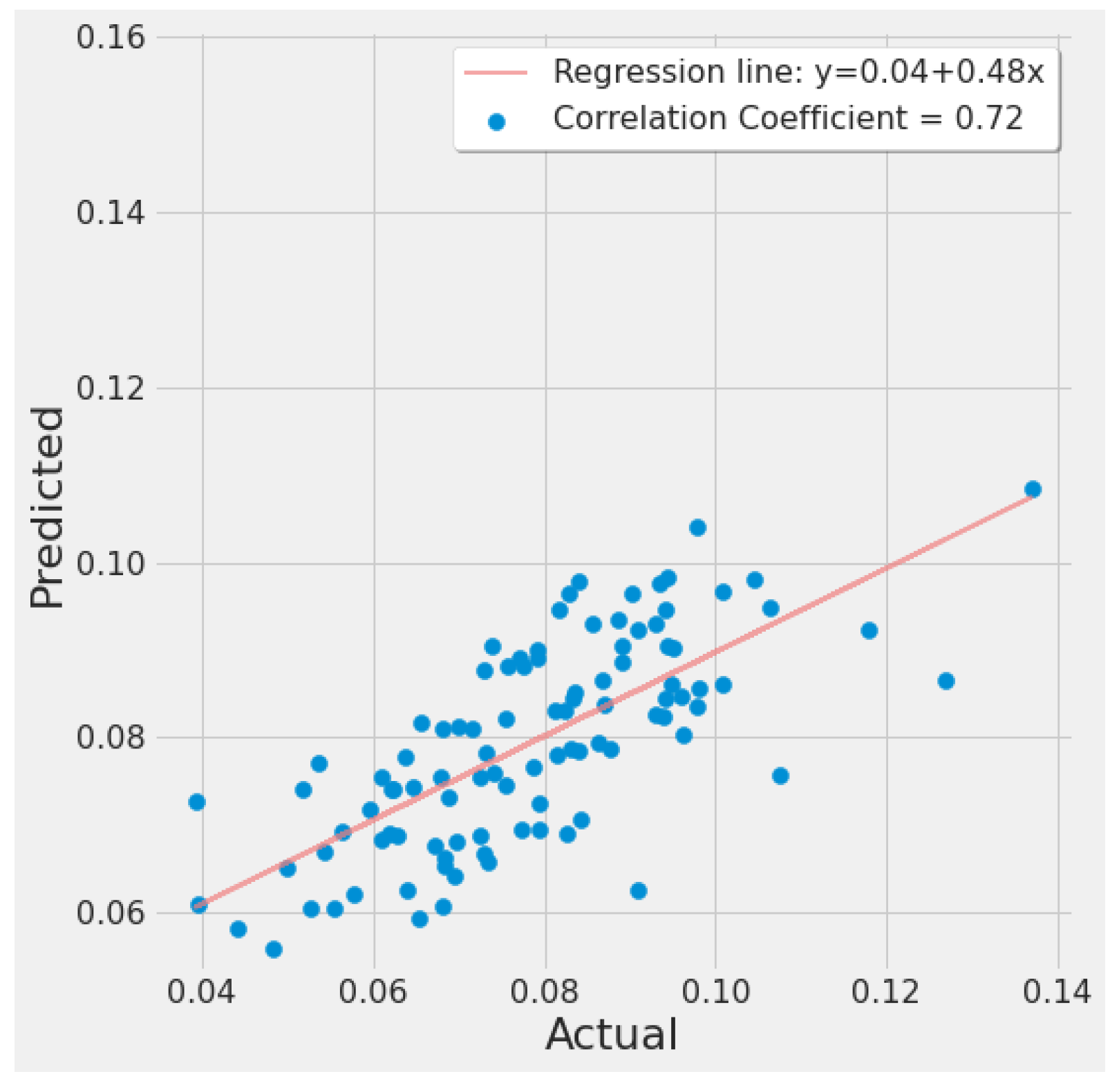
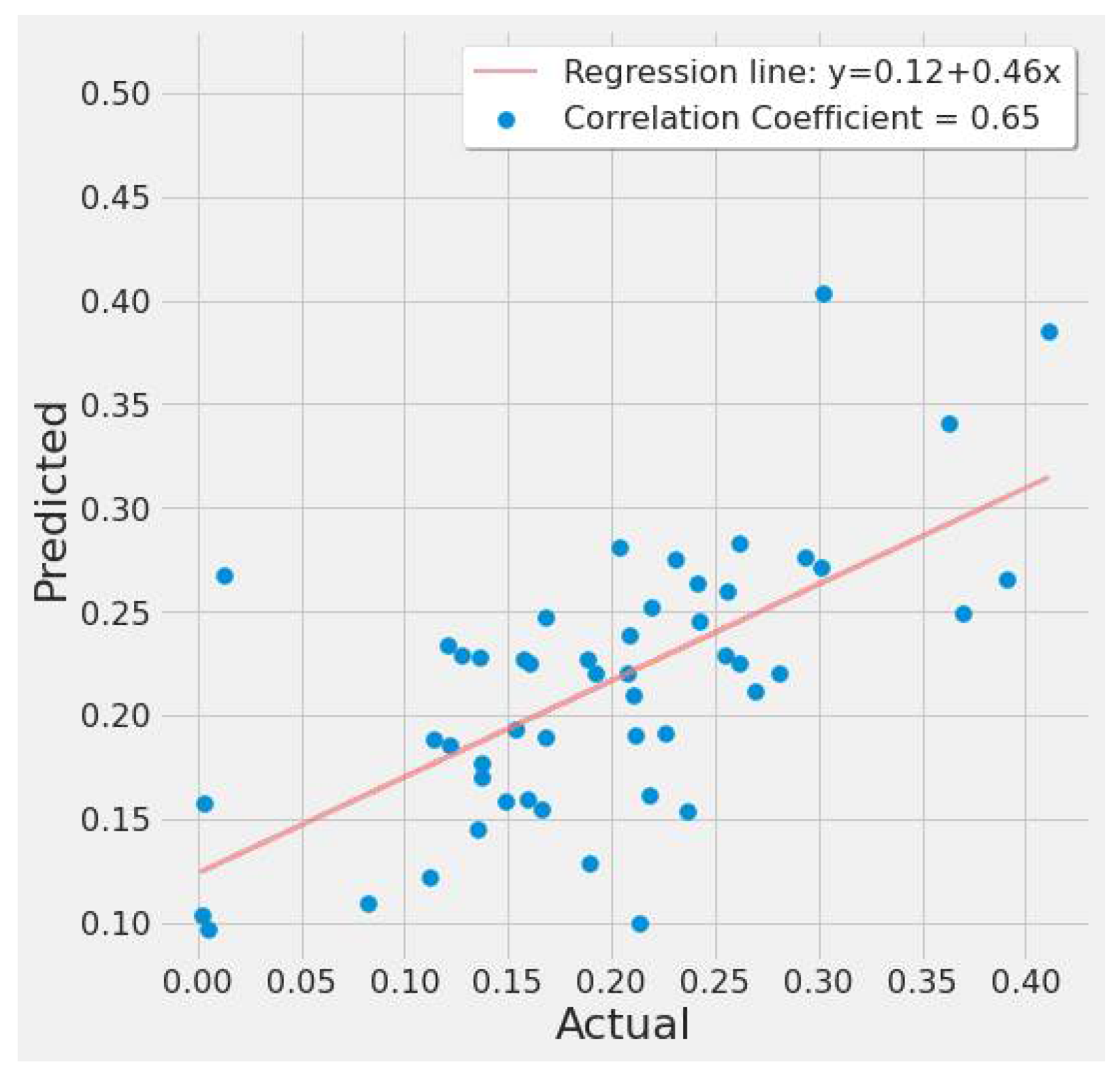
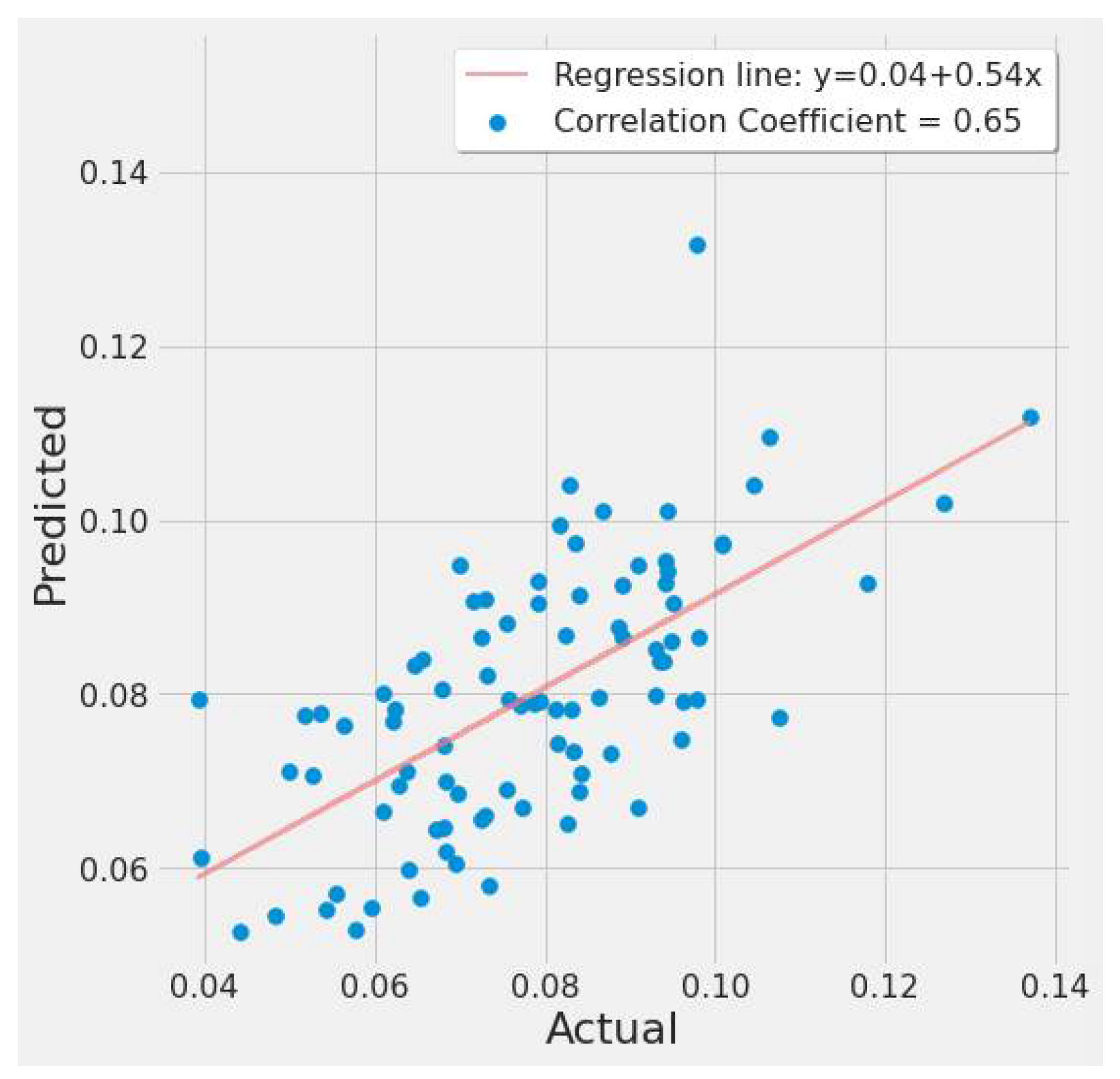
The correlation plot of actual and predicted EPA NO2 values are shown in Figure 28 and Figure 29. Both graphs reveal a moderately positive relationship, indicating a good line fit between actual and predicted values in Table 9’s #2 and #9 experiments.
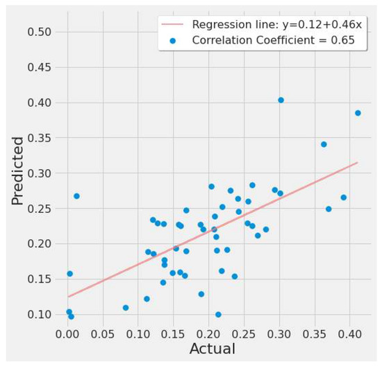
Figure 28.
XGBoost actual vs. predicted EPA NO2 correlation plot using TROPOMI and date features for the study’s first scenario.

Figure 29.
XGBoost actual vs. predicted EPA NO2 correlation plot using TROPOMI and date features for the study’s second scenario.
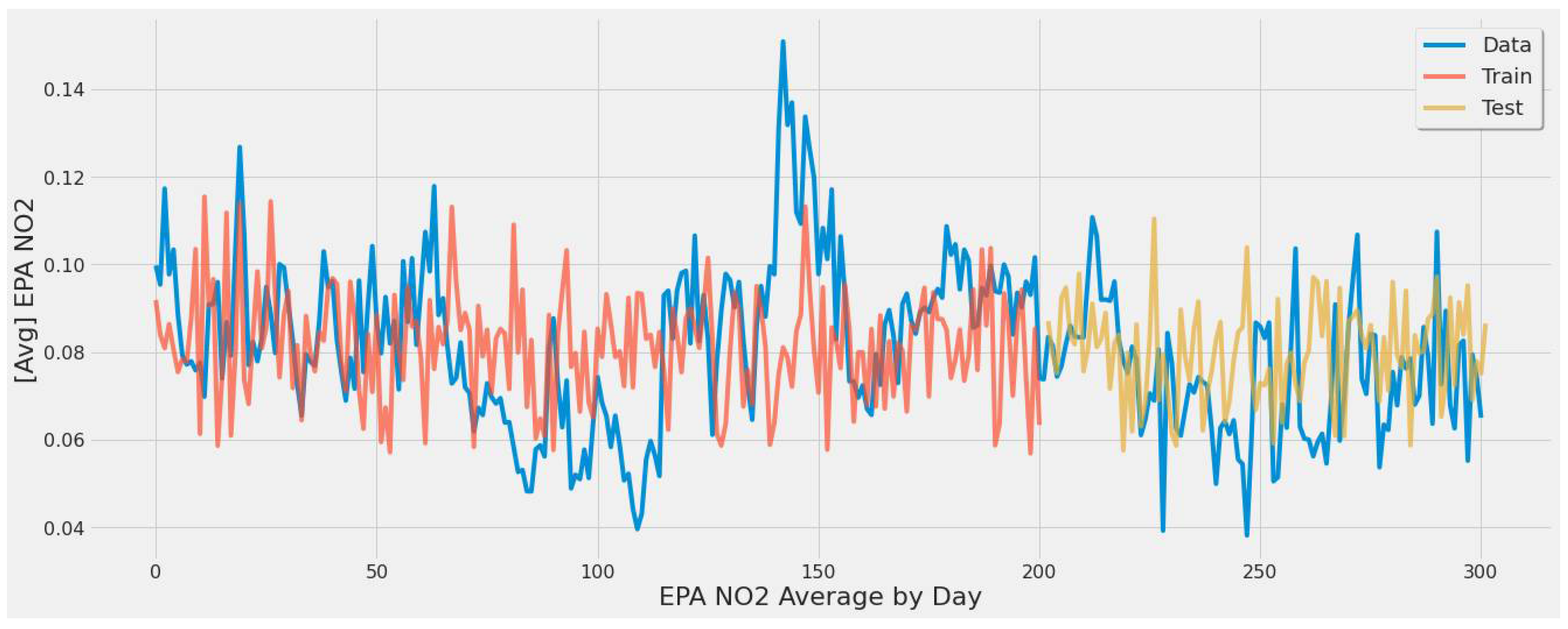
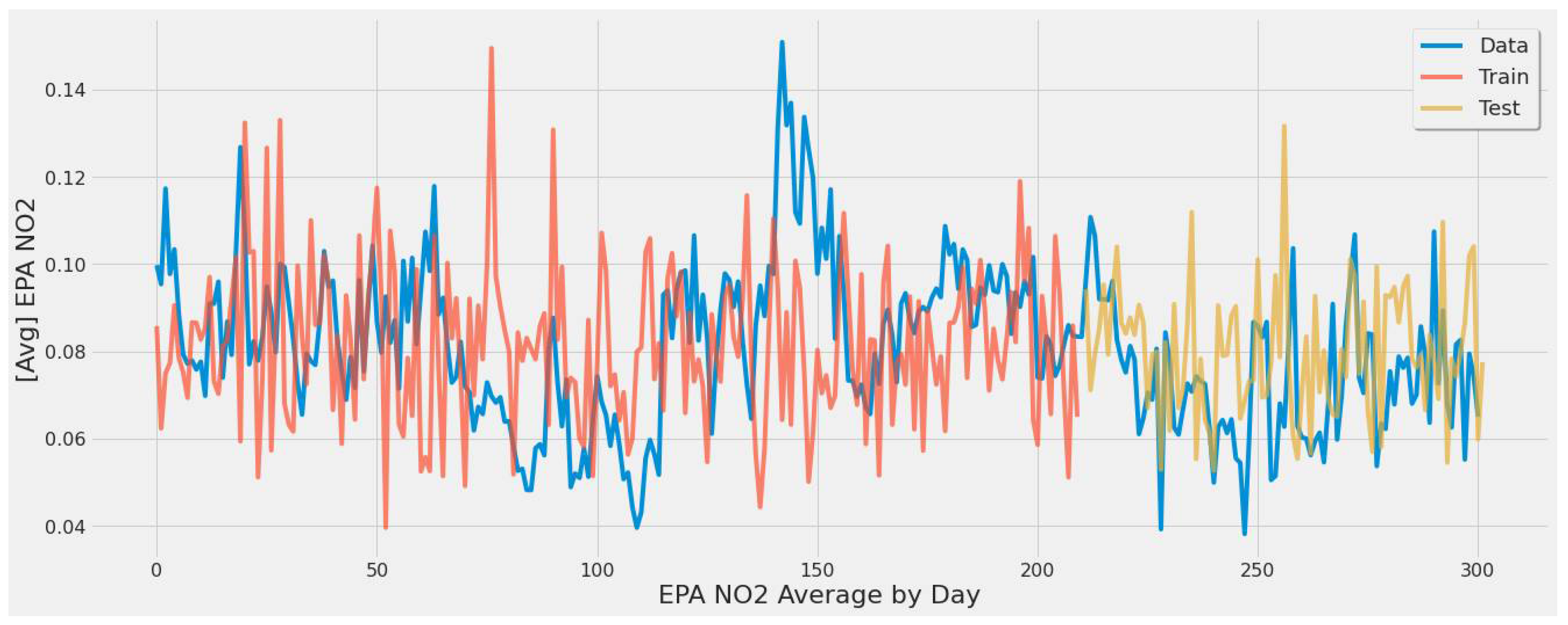
Figure 30 displays the averaged EPA NO2 by day across all 289 power plants in the U.S. Although the test set line generally matched the overall trend of actual values, there was much over and underestimation in the predicted testing values. The model underestimated certain days (day 160), but values not as extreme were captured well across the overall EPA NO2 trend. This model was biased toward a certain range of EPA NO2 values between 0.08 and 0.10.

Figure 30.
XGBoost model fit over averaged EPA NO2 values for training/testing sets throughout the year for all coal-fired power plants second scenario.
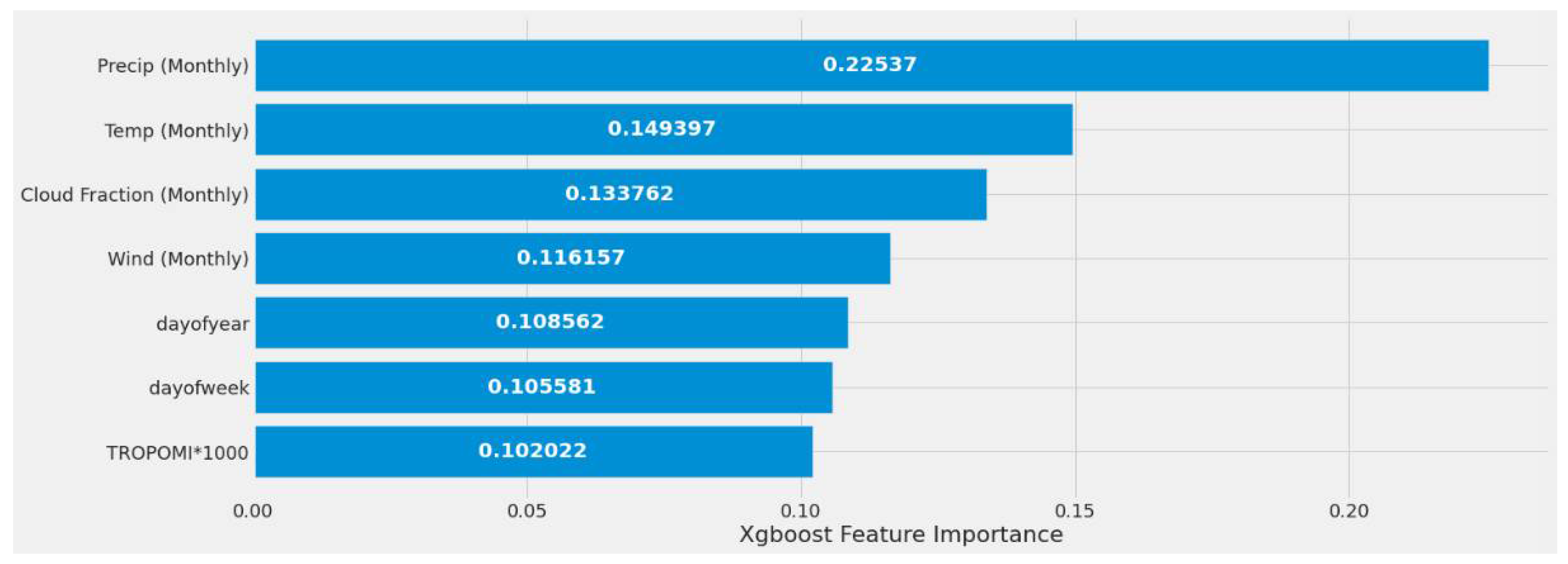
Figure 31 displays a feature importance graph that the XGBoost model deemed the most important based on the feature’s correlation score with EPA NO2. This model had different feature importance than RF and ranked MERRA-2 predictors as the most important, TROPOMI, and time features the least. This model determined that MERRA-2 features were significantly correlated with EPA NO2. Figure 31 represents experiment #2 (Table 9).

Figure 31.
XGBoost models’ feature importance using a single power plant (Alabama) dataset.
The impact of having either daily or weekly MERRA-2 data are seen in Experiments #4 through #8 (Table 9). Using weekly MERRA-2 data, the correlation between MERRA-2 and EPA NO2 improved slightly. When compared to the monthly MERRA-2 experiments, which performed significantly better, this model did not benefit from including the different MERRA-2 weekly and daily datasets.
The study’s first scenario is represented by XGBoost experiments #1, #2, and #3 (Table 9). Different feature sets produced a significant variance in MSE and error rate. Experiment #2 performed considerably better due to the inclusion of monthly MERRA-2, date features, and TROPOMI NO2. These predictors helped experiment #2 estimate EPA NO2 values 27.76% better than experiment #1 and 3.05% better than experiment #3. The second scenario findings are listed in Experiment #9 (Table 9), with the model correctly predicting 82.07% based on the error rate.
5. Discussion
5.1. Ability Assessment of ML and Remote Sensing on Predicting Single Source Emission
Most existing RS-ML research focuses on the general large-scale spatial distribution of NO2 concentration and did not explore micro-resolution single-point emission for several reasons [33]. ML can address these concerns by directly simulating the relationships between remotely sensed data and accurate ground emission sources. As shown in Section 4, at most times there was a significant correlation between TROPOMI and EPA ground observations which indicates that the relationship is very likely to help inferences from one to another. Even though the curve of TROPOMI was relatively flat compared to the EPA observations, the ups and downs in both time series resonated with each other. Regarding the emission transportation, normally the operational power plants are running constantly with short occasional breaks (e.g., EPA orders shutdown after exceeding an emission threshold), the NO2 plume should be close to the power plants and can be captured by the imagery grids even though its spatiotemporal resolution is coarse. The experiment results have validated that ML could overcome the challenges at some level and produce a reliable estimate on specific emission sources. However, certain conditions are required to allow the ML models to work in their best mode. There should be no other major second source of NO2 close by, e.g., metropolitan cities or other massive-emitter facilities. We have not experimented on the boundary of the noise sources and temporarily recommend using 100 miles to single out power plant emissions and clean the training data. In the future, with more availability of higher resolution satellite products, we will be able to use ML to predict all power plant emissions without such spatial restraint.
5.2. Spatiotemporal Pattern Discovery Using ML
Pattern recognition and generalization is a key challenge in ML application. Usually, one model working for a single power plant should be re-trained and calibrated before being applied to another power plant, because the patterns and atmosphere context are different. Observing the results in Section 4, the emission of power plants was highly correlated to the day of the year in ML model training, which is reasonable as the summer and winter are the highest peak of electricity demands and require the plants to operate for longer hours. ML captured that correlation and memorized it in its weight/decision trees. Considering the spatial variances, we also trained the models on all the power plants and compared them to the model trained only on one plant. The performance of the models trained on all power plants was relatively lower than the models trained on single plants. This means that the ML was struggling to fit on all the plants and made compromises to maintain a relatively higher accuracy on every plant. This is reasonable as at some power plants the NO2 was very high in TROPOMI, but EPA observations was lower than other plants, or vice versa. Therefore, at present, we recommend training and testing the approach on a single plant and retraining the models when transferring to a new plant. Meanwhile, it is possible to directly reuse trained models if the atmosphere context and the power plant capacity are similar, for example, two power plants located in the rural mid-west region with 3000 MWh (megawatt hour) net generation.
5.3. Long-Term Operational Capability
The stability of ML has been tested in many other applied cases and is considered trustworthy. In this study, we sought to operationalize the trained model to estimate routine emissions of all power plants as a third-party information source to help regulators to formalize and enforce environment policy. The trained model should be deployed as a service to take the newly observed TROPOMI and other input variables and output a predicted value for each power plant NO2 emission every day. The near-real-time TROPOMI products are normally ready with an average time lag of three hours after acquisition. The computation of converting format and projection, extracting values, triggering the model, and outputting the values normally takes less than ten minutes. Theoretically, the approach can refresh the NO2 estimate of the power plants within less than one day as long as TROPOMI captures a valid value on that day for the power plant location. There will be gaps due to clouds and maintenance of the satellite, which should be notified to the stakeholders via email or network platforms. Gaps of one or two days should have trivial impacts on the regular enforcement of the environmental policy. However, long gaps will have impacts which might, unfortunately, create opportunities for big emitters to violate the rules. This is an existing problem and will be further discussed in the future. Potential solutions include developing NO2 products from more reliable spectral bands that can spear through the clouds or to use third-party data sources, such as on-demand aerial-borne observations. In other words, once satellites fly over the power plants on a clear-sky day, the ML-derived NO2 emission estimates will be calculated and contained in a report and sent to environment enforcement agencies within as little as four hours.
5.4. Bias and Uncertainty
There has been much discussion and argument about the underfitting and overfitting of ML when applied to datasets with many noise sources and uncertainties, especially in high spectral passive remote sensing imagery containing noise coming from sensors or diffuse radiation. Overfitting means the model learned from noise while underfitting means the model has not fully learned the real data patterns. Unfortunately, the noise in remotely sensed data is unavoidable and sometimes cumulative in time series prediction. Many methods and calibration models have been developed for both sensor error correction and atmospheric calibration. All the remote sensing products have gone through quality control and maturity assessment. TROPOMI NRT products are processed based on the 3-dimensional global chemistry transport model and the configuration might also result in uncertainties in different locations. During operation, ESA usually upgrades their workflow occasionally and causes systematic changes in the tropospheric NO2 columns under various conditions, such as cloud-free or seriously polluted areas with small fractions. The changes will have non-trivial impacts on the ML learning process and may lead to non-usable biased estimation. It is recommended that after every major upgrade, the ML model should be re-trained on the new training data including the observations after the upgrade. The single-time-frame models, such as random forest and SVM usually do not need additional adjustments during use as the errors do not accumulate. Time series models, such as the LSTM model, do need to be adjusted or aligned after a period running to offset the accumulated biases and to bring the model status back to the correct track.
An additional cause of uncertainty is that ML models are fundamentally algorithms composed of a set of rules which involve random number generation and optimization to determine model parameters. Therefore, ML models developed on the same dataset are almost always different. The uncertainty of ML applications is a combination of uncertainties from two sources: data and knowledge.
5.5. Study and ML limitations
The findings of this study should be considered in light of some limitations:
- The data collected in this study mostly covered the essential sources for predicting NO2 emissions.
- More data volume for all data sources would have enhanced performance. The data collected was just for the year 2019, and it would have been beneficial to increase the sample size for all datasets.
- Sensor calibration and validation are integral for reliable remote sensing and proper quality of the derived variables/data. This study has ensured extraction of validated and filtered data to retrieve higher quality images of remotely sensed data. These processes are essential for better predictive modeling and, if lacking, can provide incorrect results.
- Passive remote sensing techniques (such as TROPOMI) record solar radiation reflected and emitted from Earth which can be sensitive to weather conditions, lowering their accuracy.
- The ML models and their predictive ability are the second main area of limitation.
- For our first experimental scenario, the LSTM model captured extreme values well. However, it lacked low error rate results and had weak predictive ability, similar to our early testing models.
- The inclusion of a different LSTM architecture was a response to the unsatisfactory results of the original LSTM model tested, and the stacked architecture improved the results for the most part, but not significantly.
- The nonlinear nature of the data, along with the time series element, has traditionally been a complex problem to solve due primarily to random outcomes. The study’s main goal was to take a sample of results from multiple machine learning algorithms to draw conclusions and show that estimating NO2 emissions for power plants using remote sensing data was feasible.
- The study’s experiments were rigorously conducted and validated, but they were ultimately constrained by the volume of data and the predictive performance of our models.
- Additional data sources correlated with NO2 emissions and better remote sensing resolution could considerably improve the results in the future.
6. Conclusions and Future Work
This paper utilized ML to simulate the non-linear relationships and memorize the hidden patterns between remote sensing data and EPA ground observation to estimate emissions from power plants. Several representative ML algorithms have been tested. Compared to traditional techniques, such as numeric modeling and rule-based workflow processing systems, ML has fewer restrictions, such as requiring no initial field conditions, equation coefficient adjustments, expensive computation costs, and no unrealistic assumptions. Future iterations of this study can better use ML models rather than linear regression as their baseline models to achieve higher accuracy and better reliability. This study collected data from multiple data sources including TROPOMI NRT NO2 products, EPA eGRID ground monitoring network data, and NASA MERRA weather data. The training data used TROPOMI and MERRA variables as inputs and EPA emission data as outputs. It covered more than two hundred power plants across the United States. However, due to the relatively coarse spatial resolution of remote sensing data at present (TROPOMI has 7 × 3.5 km before August 2019 and a higher resolution of 3.5 × 5.5 km currently), the NO2 reflected in remote sensing data possibly did not exclusively come from power plants, especially in urban regions. To exclude impacts from other emission sources, we initially chose those power plants located in the rural regions for initial tests. The results showed that ML is capable of correctly detecting the changing trends of NO2 emission by power plants. They confirm that ML is very promising in identifying a reliable value range for specific ground emission sources simply based on remotely sensed daily data (if the remote sensing data has no gaps, such as clouds).
In the future, we will continue to explore different combinations of input variables and tune hyperparameters to improve the accuracy of the trained ML models. More data sources, such as new satellite observations, will enable experiments to increase the spatiotemporal coverage of remote sensing to refine prediction. Right now, the model is not spatially reusable, and we will explore the options to transfer and reuse the models in new power plants in other regions or countries. Another important focus of research is to deploy the model into cloud servers and to start to provide operational services to stakeholders as an alternative information source to monitor coal-fired power plants.
Author Contributions
Conceptualization, Z.S. and D.T.; methodology, Z.S.; software, Z.S.; validation, A.A. and Z.S.; formal analysis, A.A. and Z.S.; investigation, A.A. and Z.S.; resources, Z.S. and D.T.; data curation, Z.S., D.T. and A.A.; writing—original draft preparation, A.A. and Z.S.; writing—review and editing, A.A., Z.S.; visualization, A.A.; supervision, Z.S.; project administration, Z.S.; funding acquisition, Z.S. All authors have read and agreed to the published version of the manuscript.
Funding
This research was funded by NASA ACCESS (#80NSSC21M0028), NASA Applied Science (#17-HAQ17-0044), NSF Geoinformatics (#EAR-1947893).
Acknowledgments
Thanks to Microsoft for providing the Azure computing resources to carry out the initial data processing. Thanks, Zack Chester, for initially collecting and processing the data. Thanks to all the authors of the open-source software we have used during this research.
Conflicts of Interest
The authors declare no conflict of interest.
References
- Nitrogen Oxides (NOx), Why and How They Are Controlled.57. Available online: https://www3.epa.gov/ttn/catc/dir1/fnoxdoc.pdf (accessed on 15 December 2021).
- Srivastava, R.K.; Hall, R.E.; Khan, S.; Culligan, K.; Lani, B.W. Nitrogen Oxides Emission Control Options for Coal-Fired Electric Utility Boilers. J. Air Waste Manag. Assoc. 2005, 55, 1367–1388. [Google Scholar] [CrossRef] [PubMed] [Green Version]
- US EPA, O. Cleaner Power Plants. Available online: https://www.epa.gov/mats/cleaner-power-plants (accessed on 15 December 2021).
- Geostationary Satellite Constellation for Observing Global Air Quality: Geophysical Validation Needs. Available online: https://ceos.org/document_management/Publications/Publications-and-Key-Documents/Atmosphere/GEO_AQ_Constellation_Geophysical_Validation_Needs_1.1_2Oct2019.pdf (accessed on 15 December 2021).
- Beirle, S.; Borger, C.; Dörner, S.; Eskes, H.; Kumar, V.; de Laat, A.; Wagner, T. Catalog of NOx Emissions from Point Sources as Derived from the Divergence of the NO2 Flux for TROPOMI. Earth Syst. Sci. Data 2021, 13, 2995–3012. [Google Scholar] [CrossRef]
- Van der A, R.J.; de Laat, A.T.J.; Ding, J.; Eskes, H.J. Connecting the Dots: NOx Emissions along a West Siberian Natural Gas Pipeline. npj Clim. Atmos. Sci. 2020, 3, 1–7. [Google Scholar] [CrossRef] [Green Version]
- Hedley, J.; Russell, B.; Randolph, K.; Dierssen, H. A Physics-Based Method for the Remote Sensing of Seagrasses. Remote Sens. Environ. 2016, 174, 134–147. [Google Scholar] [CrossRef]
- Crosman, E. Meteorological Drivers of Permian Basin Methane Anomalies Derived from TROPOMI. Remote Sens. 2021, 13, 896. [Google Scholar] [CrossRef]
- Lorente, A.; Boersma, K.F.; Eskes, H.J.; Veefkind, J.P.; van Geffen, J.H.G.M.; de Zeeuw, M.B.; Denier van der Gon, H.A.C.; Beirle, S.; Krol, M.C. Quantification of Nitrogen Oxides Emissions from Build-up of Pollution over Paris with TROPOMI. Sci. Rep. 2019, 9, 20033. [Google Scholar] [CrossRef]
- Beirle, S.; Borger, C.; Dörner, S.; Li, A.; Hu, Z.; Liu, F.; Wang, Y.; Wagner, T. Pinpointing Nitrogen Oxide Emissions from Space. Sci. Adv. 2019, 5, eaax9800. [Google Scholar] [CrossRef] [Green Version]
- Ialongo, I.; Virta, H.; Eskes, H.; Hovila, J.; Douros, J. Comparison of TROPOMI/Sentinel-5 Precursor NO2 Observations with Ground-Based Measurements in Helsinki. Atmos. Meas. Tech. 2020, 13, 205–218. [Google Scholar] [CrossRef] [Green Version]
- Yu, M.; Liu, Q. Deep Learning-Based Downscaling of Tropospheric Nitrogen Dioxide Using Ground-Level and Satellite Ob-servations. Sci. Total Environ. 2021, 773, 145145. [Google Scholar] [CrossRef]
- Yang, G.; Wang, Y.; Li, X. Prediction of the NOx Emissions from Thermal Power Plant Using Long-Short Term Memory Neural Network. Energy 2020, 192, 116597. [Google Scholar] [CrossRef]
- Karim, R.; Rafi, T.H. An Automated LSTM-Based Air Pollutant Concentration Estimation of Dhaka City, Bangladesh. Int. J. Eng. Inf. Syst. 2020, 4, 88–101. [Google Scholar]
- Kristiani, E.; Kuo, T.-Y.; Yang, C.-T.; Pai, K.-C.; Huang, C.-Y.; Nguyen, K.L.P. PM2.5 Forecasting Model Using a Combination of Deep Learning and Statistical Feature Selection. IEEE Access 2021, 9, 68573–68582. [Google Scholar] [CrossRef]
- Abimannan, S.; Chang, Y.-S.; Lin, C.-Y. Air Pollution Forecasting Using LSTM-Multivariate Regression Model. In Proceedings of the Internet of Vehicles, Technologies and Services Toward Smart Cities, Kaohsiung, Taiwan, 18–21 November 2019; Hsu, C.-H., Kallel, S., Lan, K.-C., Zheng, Z., Eds.; Springer International Publishing: Cham, Switzerland, 2020; pp. 318–326. [Google Scholar]
- Georgoulias, A.K.; Boersma, K.F.; van Vliet, J.; Zhang, X.; Zanis, P.; Laat, J. Detection of NO2 Pollution Plumes from Individual Ships with the TROPOMI/S5P Satellite Sensor. Environ. Res. Lett. 2020, 15, 124037. [Google Scholar] [CrossRef]
- Si, M.; Du, K. Development of a Predictive Emissions Model Using a Gradient Boosting Machine Learning Method. Environ. Technol. Innov. 2020, 20, 101028. [Google Scholar] [CrossRef]
- Zhan, Y.; Luo, Y.; Deng, X.; Zhang, K.; Zhang, M.; Grieneisen, M.L.; Di, B. Satellite-Based Estimates of Daily NO2 Exposure in China Using Hybrid Random Forest and Spatiotemporal Kriging Model. Environ. Sci. Technol. 2018, 52, 4180–4189. [Google Scholar] [CrossRef]
- Chen, T.-H.; Hsu, Y.-C.; Zeng, Y.-T.; Candice Lung, S.-C.; Su, H.-J.; Chao, H.J.; Wu, C.-D. A Hybrid Kriging/Land-Use Regres-sion Model with Asian Culture-Specific Sources to Assess NO2 Spatial-Temporal Variations. Environ. Pollut. 2020, 259, 113875. [Google Scholar] [CrossRef] [PubMed]
- Novotny, E.V.; Bechle, M.J.; Millet, D.B.; Marshall, J.D. National Satellite-Based Land-Use Regression: NO2 in the United States. Environ. Sci. Technol. 2011, 45, 4407–4414. [Google Scholar] [CrossRef] [PubMed]
- Wong, P.-Y.; Su, H.-J.; Lee, H.-Y.; Chen, Y.-C.; Hsiao, Y.-P.; Huang, J.-W.; Teo, T.-A.; Wu, C.-D.; Spengler, J.D. Using Land-Use Machine Learning Models to Estimate Daily NO2 Concentration Variations in Taiwan. J. Clean. Prod. 2021, 317, 128411. [Google Scholar] [CrossRef]
- El Khoury, E.; Ibrahim, E.; Ghanimeh, S. A Look at the Relationship Between Tropospheric Nitrogen Dioxide and Aerosol Optical Thickness Over Lebanon Using Spaceborne Data of the Copernicus Programme. In Proceedings of the 2019 Fourth International Conference on Advances in Computational Tools for Engineering Applications (ACTEA), Beirut, Lebanon, 3–5 July 2019; pp. 1–6. [Google Scholar]
- Lin, C.-A.; Chen, Y.-C.; Liu, C.-Y.; Chen, W.-T.; Seinfeld, J.H.; Chou, C.C.-K. Satellite-Derived Correlation of SO2, NO2, and Aerosol Optical Depth with Meteorological Conditions over East Asia from 2005 to 2015. Remote Sens. 2019, 11, 1738. [Google Scholar] [CrossRef] [Green Version]
- Superczynski, S.D.; Kondragunta, S.; Lyapustin, A.I. Evaluation of the Multi-Angle Implementation of Atmospheric Correc-tion (MAIAC) Aerosol Algorithm through Intercomparison with VIIRS Aerosol Products and AERONET. J. Geophys. Res. Atmos. 2017, 122, 3005–3022. [Google Scholar] [CrossRef] [Green Version]
- Zhao, X.; Griffin, D.; Fioletov, V.; McLinden, C.; Cede, A.; Tiefengraber, M.; Müller, M.; Bognar, K.; Strong, K.; Boersma, F.; et al. Assessment of the Quality of TROPOMI High-Spatial-Resolution NO2 Data Products in the Greater Toronto Area. Atmos. Meas. Tech. 2020, 13, 2131–2159. [Google Scholar] [CrossRef]
- Verhoelst, T.; Compernolle, S.; Pinardi, G.; Lambert, J.-C.; Eskes, H.J.; Eichmann, K.-U.; Fjæraa, A.M.; Granville, J.; Niemeijer, S.; Cede, A.; et al. Ground-Based Validation of the Copernicus Sentinel-5P TROPOMI NO2 Measurements with the NDACC ZSL-DOAS, MAX-DOAS and Pandonia Global Networks. Atmos. Meas. Tech. 2021, 14, 481–510. [Google Scholar] [CrossRef]
- Wang, C.; Wang, T.; Wang, P.; Rakitin, V. Comparison and Validation of TROPOMI and OMI NO2 Observations over China. Atmosphere 2020, 11, 636. [Google Scholar] [CrossRef]
- The Aura Mission. Available online: https://aura.gsfc.nasa.gov/omi.html (accessed on 14 December 2021).
- Khatibi, A.; Krauter, S. Validation and Performance of Satellite Meteorological Dataset MERRA-2 for Solar and Wind Applications. Energies 2021, 14, 882. [Google Scholar] [CrossRef]
- Merrill, R. Procedure 1. Quality Assurance Requirements for Gas Continuous Emission Monitoring Systems Used for Compliance Determination; EPA: Washington, DC, USA, 2020; 9p.
- US EPA, O. National Emissions Inventory (NEI). Available online: https://www.epa.gov/air-emissions-inventories/national-emissions-inventory-nei (accessed on 10 December 2021).
- Sun, Z.; Sandoval, L.; Crystal-Ornelas, R.; Mousavi, S.M.; Wang, J.; Lin, C.; Cristea, N.; Tong, D.; Carande, W.H.; Ma, X.; et al. A Review of Earth Artificial Intelligence. Comput. Geosci. 2022, 159, 105034. [Google Scholar] [CrossRef]
Publisher’s Note: MDPI stays neutral with regard to jurisdictional claims in published maps and institutional affiliations. |
© 2022 by the authors. Licensee MDPI, Basel, Switzerland. This article is an open access article distributed under the terms and conditions of the Creative Commons Attribution (CC BY) license (https://creativecommons.org/licenses/by/4.0/).

