Article

The Forest Change Footprint of the Upper Indus Valley, from 1990 to 2020

1
State Key Laboratory of Resources and Environmental Information System, Institute of Geographic Sciences and Natural Resources Research, Chinese Academy of Sciences, Beijing 100101, China
2
University of Chinese Academy of Sciences, Beijing 100049, China
3
China-Pakistan Earth Science Research Center, Islamabad 45320, Pakistan
4
Jiangsu Center for Collaborative Innovation in Geographical Information Resource Development and Application, Nanjing 210023, China
*
Author to whom correspondence should be addressed.
Remote Sens. 2022, 14(3), 744; https://doi.org/10.3390/rs14030744
Submission received: 20 December 2021 / Revised: 22 January 2022 / Accepted: 3 February 2022 / Published: 5 February 2022

Abstract

:
The upper Indus Valley is the most important and vulnerable water tower in the South Asian subcontinent, which provides a vital water supply for 230 million people in the basin. Forests play an important role in water conservation in this region, and the security of upstream forests forms the foundation downstream water and food security. However, a big challenge is to effectively monitor the dynamics of the forest in this region. Thus, we used the LandTrendr spectral-temporal segmentation algorithm combined with 8203 scenes of multi-source remote sensing data to study the forest change footprint in the upper Indus Valley. The overall accuracy of LandTrendr extraction for forest disturbance and recovery was 86.01%, and the Kappa coefficient was 0.73. The results showed the following: (1) From 1990 to 2020, the area of forest recovery was 1.01% more than that of disturbance, 70% of disturbance occurred between 1990 and 2001, and 60% of recovery occurred between 1999 and 2012. (2) Although the overall trend of forest disturbance and recovery was balanced, there were significant differences in forest management status among the different regions. Nepal has the highest forest stability, India has the largest area of forest disturbance, and Pakistan and China have the largest areas of forest recovery. (3) India’s Himachal Pradesh and Jammu and Kashmir are the two provinces with the largest disturbed areas, primarily due to grazing, fires, and commercial tree planting. Pakistan’s North-West Frontier, Azad Kashmir, and China’s Tibet Ali region were major contributors to the recovery, which was driven by afforestation policies in both countries. This study provides an important data base and monitoring method for planning land and forest use in Indus Valley countries, protecting fragile environments, and promoting policies for the Sustainable Development Goals.

1. Introduction

Forests are the main component of terrestrial ecosystem and the largest “carbon pool” on land, which plays an important role in regulating climate and mitigating global warming [1]. Monitoring forest disturbance and recovery has received abundant attention over the past few decades, especially to identify the important role of forests in curbing climate warming and achieving “carbon neutrality” [2]. The United Nations Sustainable Development Goal (SDG) 15 calls for the protection, restoration, and promotion of the sustainable use of terrestrial ecosystems and sustainable management of forests as well as a series of assessment indicators [3]. Forest disturbance is the main factor that affects forest growth, structure, and function. This disturbance is largely due to the degradation and disappearance of forests caused by environmental changes such as drought, hurricanes, geological disasters, and various human activities [4,5]. Forest recovery involves a series of favorable conditions that can promote the growth of forests, including internal and external factors. In areas with more favorable climatic conditions, forest disturbances can be recovered through succession of forest communities or internal self-regulation of ecosystems [6]. In high latitude and ecologically fragile areas, the implementation of forest protection policies plays a positive role in forest recovery [7,8]. Using the Landsat pixel scale, forest disturbance was defined as partial or complete disappearance of the forest canopy. Forest recovery is defined as the inverse ratio of forest loss, which represents an increase in forest cover of the tree canopy [9].
The upper Indus Valley is one of the most critical water towers in the world [10], and ecosystem security in this region is directly linked to the welfare of 230 million individuals downstream. The Karakoram, Hindu Kush, Ladakh, and Himalayas in the upper reaches form diverse forest ecosystems, which are important carbon sinks and water conservation areas. The security of forest ecosystems is related to the security of water and agricultural resources in the Indus Valley basin. However, forest disturbances in this region have been a concern in recent decades. Studies have shown that the annual deforestation rate in this area reaches 2.2% [11]. A previous study by Rashid et al. (2017) showed that the evergreen broad-leaved forest in Kashmir was degraded, and aboveground biomass and carbon storage were lost, thereby adversely affecting carbon fixation in this region [12]. There is evidence that forests in the upper Indus Valley were destroyed, and severe forest disturbances devastated the stability of the original forest ecosystem, leading to catastrophic floods in 1992 and 2010. In response to these problems, the governments of relevant countries have issued several commercial logging bans, but this has not prevented the loss of upstream forest areas. The rate of deforestation and loss of total forest area in this region are still higher than the global average [11,13]. Thus, it is urgent to obtain information on the disturbance and recovery of forests in recent decades through various monitoring methods to provide a reference for the formulation of forest policies in this region.
Forest disturbance and recovery information can be obtained through many technical means such as regular field surveys of forest resources. China, Canada, and Finland have developed relatively complete forest resource survey techniques, but these require higher human and economic costs. The upper Indus Valley includes five countries, and it is difficult to organize forest surveys and obtain forest disturbance and recovery data for all countries. Remote sensing technology is currently considered the most effective and lowest cost method, providing spatiotemporal awareness of forest change on multiple scales [14,15]. The principle of remote sensing technology for monitoring disturbance and recovery is to track the change information of the vegetation canopy spectrum in a time-series image. When the band or index representing the vegetation canopy suddenly or gradually exceeds a certain threshold, the forest is considered disturbed or recovered [16]. Time-series images provide important, consistent, and continuous data sources for the acquisition of forest footprint information in forest-covered areas. Early forest change monitoring based on remote sensing mainly came from the comparative analysis of the interpretation results of two or more temporal remote sensing images. However, because of the limitation of the timeliness of interpretation of samples and other reasons, such methods generally span many years, such as 5 or 10 years, ignoring the short-interval footprint information in the process of forest change, and it is difficult to achieve continuous monitoring of forest change information from a large area.
In the upper Indus Valley, Joshi et al. (2014) interpreted images of the central Himalaya in 1979, 1999, and 2009 by means of artificial visual interpretation, in which forest stands are reduced and forest areas are affected by degradation and isolation [17]. To obtain information on forest loss in the Himalayas, Qamer et al. (2016) used remote sensing images during two time periods from 1990 to 2000 and 2000 to 2010 [18]. Owing to the limitation of computing power or samples, these methods did not describe the forest loss footprint information in detail, and the images of the three periods could not dynamically restore the process of forest change over 21 years. However, most of these were short-term and partial studies, making it difficult to create an overall assessment of the forest status of the entire upper Indus Valley. With the accumulation of remote sensing images and the enhancement of data computing capability, forest change monitoring has gradually developed into a time-series image combined with a change detection algorithm. Since the release of Earth big data computing platforms, such as Google Earth Engine (GEE), increased data computing power has enabled forest change monitoring to use higher spatial resolution data. [19]. In recent years, the big data cloud computing platform for Earth observation has increasingly integrated interference and recovery monitoring algorithms. This includes the vegetation change tracker [20], breaks for additive seasonal and trend [21], vegetation regeneration and disturbance estimates over time [22], continuous change detection and classification [23], and continuous monitoring of land disturbance [24]. These algorithms are widely used in forest event monitoring, such as forest fires, deforestation, and degradation, and are important for recognizing long-term changes in forests.
Based on this background, this research intends to combine Landsat time-series imagery and Earth observation big data cloud computing platform GEE to carry out forest disturbance and recovery monitoring research in the upper Indus Valley. The main objectives include the following: (1) combining the time-spectral segmentation algorithm LandTrendr to obtain the forest change footprint in the upper Indus Valley from 1990 to 2020; and (2) analysis of the results of forest disturbance and recovery to obtain the spatiotemporal cognition of the forest change footprint in the upper Indus Valley.

2. Materials and Methods

2.1. Study Area

The Indus River is a major river in Central Asia and an important source of agricultural irrigation that feeds more than 230 million people. The Indus Valley, ranging from 24° N to 37° N and from 66° E to 82° E (Figure 1), has a diverse geographical environment, covering an area of 618,580.35 km2. It borders the Karakoram Mountains and Himalayas to the northeast, the Thar Desert in India to the southeast, the Hindu Kush Mountains in Afghanistan to the northwest, the Baluchistan Plateau to the southwest, and the Arabian Gulf to the south. The Indus Valley has a subtropical climate, characterized by a distinct monsoon climate. However, owing to the influence of the high mountains in the northeast, the climate is usually between dry and semi-dry, tropical, and subtropical. The year is divided into four seasons.
The upper Indus Valley is the intersection of many mountain ranges, and the complex geographical environment has led to the development of a variety of forest ecosystems. The natural vegetation mainly includes coniferous forests (subalpine forests, arid temperate forests, humid temperate forests, and subtropical pine forests), shrub forests (arid subtropical broad-leaved forests and arid tropical thorn forests), economic forests, and shelter forests. The forests are widely distributed between 500 and 5500 m elevation, and 90% of the forests are located above 1500 m.
According to a report from the Worldwide Fund for Nature, the population boom coupled with poverty and a lack of awareness have led to illegal and unsustainable logging, excessive logging for fuel and charcoal, and increased small-scale agriculture, which continue to reduce the amount of forest cover in the upper Indus Valley. In addition, forest fires, natural disasters, climate change, pests, and diseases further contribute to the degradation and disappearance of forests [25].

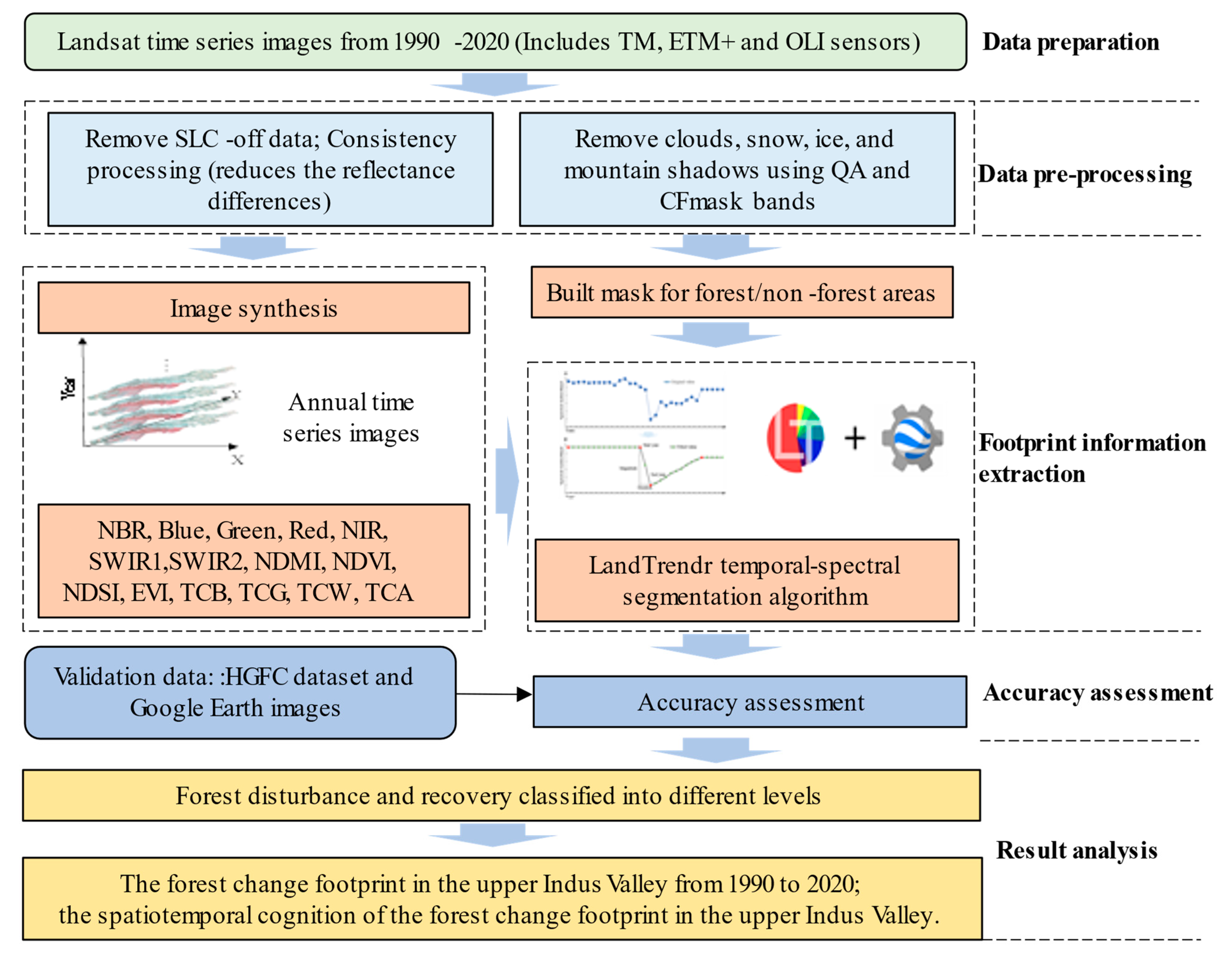
2.2. Data Preprocessing

Table 1 shows the sources and descriptions of multi-source remote sensing data used in this study. Landsat time-series data were used from the United States Geological Survey (USGS), including thematic mapper (TM), enhanced thematic mapper (ETM), and operational land imager (OLI) sensors. The data have the advantages of having high resolution, a short revisit cycle, and easy access and processing. GEE was used as the main data processing platform, which provided access to the atmospheric correction surface reflectance data of all Landsat sensors. We connected all available remote sensing images of vegetation growth season on the GEE platform from July 15 to October 1, which can effectively avoid images caused by seasonal snow in high-altitude mountainous areas. Landsat 7 ETM+ scan line corrector failure (SLC-off) images with data gaps were removed. A total of 8203 remote sensing images were used in this study. In order to reduce the influence of the difference in reflection wavelength between ETM+ and OLI sensors on the results, the harmonic function from OLI to ETM+ was used to process the data consistently [26]. In the high mountains of South Asia, clouds, snow, ice, and mountain shadows have a serious impact on the results of forest change monitoring. We used the image quality assessment band (QA) and the CFMask algorithm to generate masks to remove these four types of elements, and the annual image was generated by the median synthesis method [27]. According to the statistics obtained from annual synthetic images, cloud-free observation has been achieved in 90% of the forest for more than 20 years, and the average cloud-free observation time for each pixel was 25.5 years from 1990 to 2010. The annual synthetic images meet the requirements for LandTrendr algorithm fitting.

2.3. Forest Change Footprint Information Extraction

Figure 2 shows the workflow for obtaining forest change footprint information. This process mainly includes data collection and processing, mask construction, algorithm segmentation, different levels of disturbance and recovery classification, and accuracy assessment.

2.3.1. Built Mask for Forest/Non-Forest Areas

The forest mask can effectively avoid the influence of cultivated land and dense grassland on LandTrendr segmentation results. In this study, the forest area needed to be a maximum union of the forest distribution from 1990 to 2020, which cannot be achieved by using remote sensing images or datasets of a single time phase.
We obtained all available remote sensing images for July 1 to October 1 from 1990 to 2020, and based on the forest extract rule, a normalized difference vegetation index (NDVI) > 0.6 and short-waved infrared radiation (SWIR) < 0.1 generated the annual forest distribution area. Zhu et al. (2012) showed that the NDVI of the forest growth season is always above 0.6, but sometimes other vegetation types, such as crops, grass, and shrubs, could also have an overall forest NDVI value above 0.6. Since forests are generally dark in the SWIR band compared to other vegetation types, a surface reflectance threshold of 0.1 in the overall band 7 excludes other vegetation types that may have high NDVI values [14,28]. The maximum forest union from 1990 to 2020 showed that there was a total forest area of 46,192.25 km2 in the study area, with a forest coverage fraction of 7.47%.

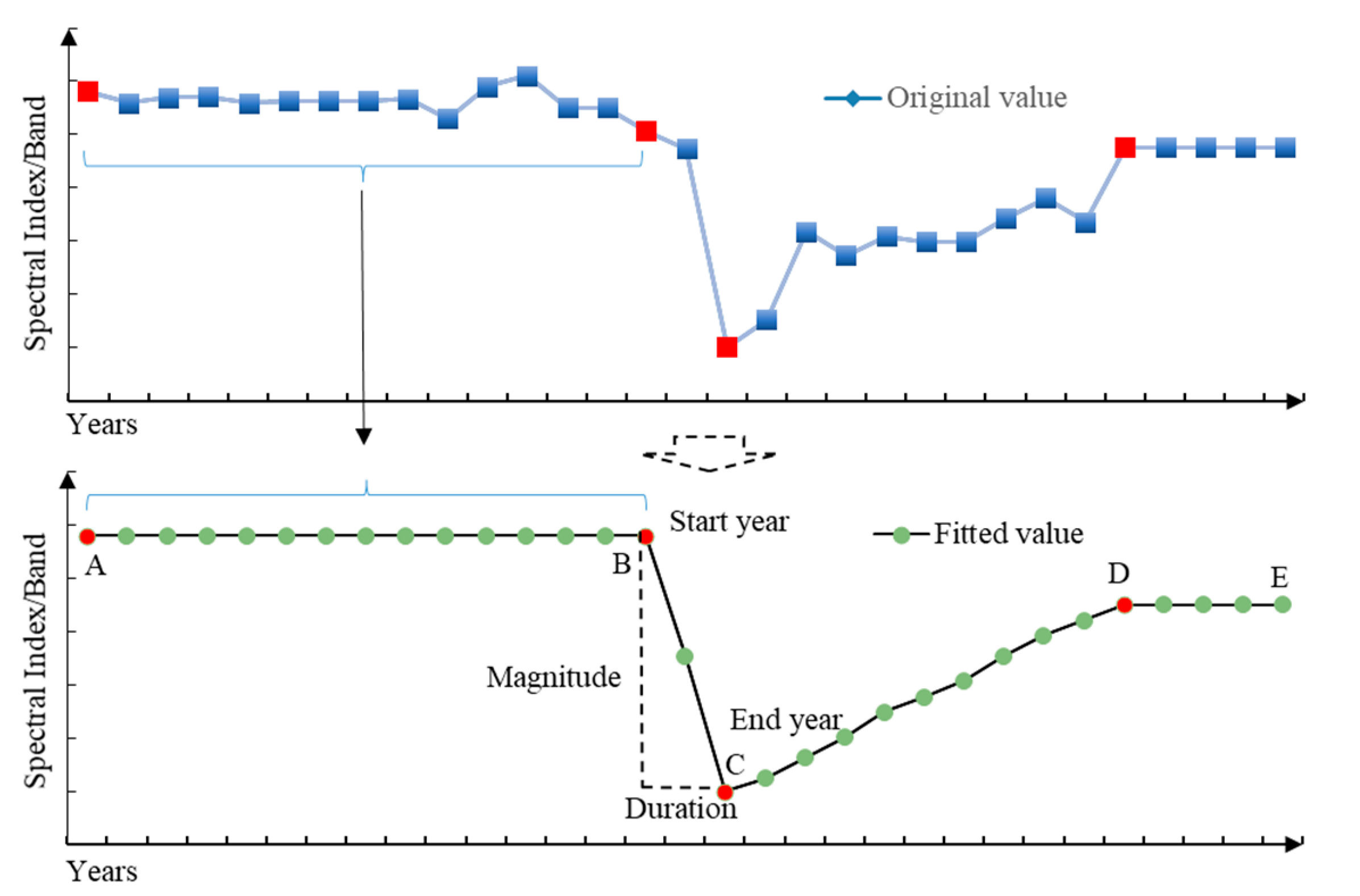
2.3.2. Detection Methods for Forest Disturbance and Recovery

LandTrendr is a set of spectral-temporal segmentation algorithms based on remote sensing image pixels that are useful for change detection in a time series of moderate-resolution satellite imagery. The time segmentation algorithm is considered an effective method for detecting forest disturbance and recovery. The trajectory of the generated spectral time-series data had almost no interannual signal noise [29]. The algorithm uses a time segmentation strategy based on regression and a point-to-point fitting spectral index as a time function, allowing for the capture of slow-evolving processes such as recovery and unexpected events [30]. Interactive Data Language (IDL) initially implemented LandTrendr, and later Google engineers ported LandTrendr to the GEE platform [19,31].
The GEE framework nearly eliminates the onerous data management and image preprocessing aspects of the IDL implementation. LandTrendr combined with GEE also simplifies tedious data management and image preprocessing by directly accessing geospatial datasets. Figure 3 shows the process of the LandTrendr algorithm for extracting forest disturbances. The discrete original value of the spectral index or band was divided into a series of straight lines and breakpoints. From the segmentation results, the start year, end year, duration, and magnitude of the spectral index or band of forest disturbance can be easily obtained.
The LandTrendr algorithm requires a series of surface reflectance bands and spectral indices as inputs when performing spectral-time segmentation. The first band or index was used for the main segmentation, and the other bands were used for fitting to supplement the best results. Cohen et al. (2018) showed that using the 13 bands and indices in Table 2 can effectively reduce the error rate of the LandTrendr segmentation [32]. Table 2 shows the bands and indices used in this study. After obtaining the segmentation results from LandTrendr, we filtered the segmentation results using a forest mask to remove the effects of dense grassland and cropland.

2.3.3. Classification of Forest Disturbance and Recovery Levels

Three levels of disturbance and recovery were classified to further study the extent of forest disturbance and recovery (Table 3). In the segmentation results of the LandTrendr algorithm, the “magnitude” band records the variation amplitude of disturbance and recovery in different years. Different levels of disturbance and recovery were obtained by reclassifying this band. Referring to previous study [41], we obtained the thresholds of disturbance and recovery using the visual interaction method between classification results and high-resolution remote sensing images from Google Earth.
Serious disturbance and strong recovery categories indicate distinct processes of forest change, such as clear-cutting or barren afforestation. Moderate disturbance, moderate recovery, light disturbance, and light recovery may be changes in forest growth trends, such as varying levels of forest degradation or the growth process from young forests to mature forests [41].

2.3.4. Accuracy Assessment

In this study, we validated the forest disturbance and recovery results using two data sources: HGFC datasets and Google Earth images. The validation data were classified into four categories: disturbance, recovery, and both disturbance and recovery (disturbance + recovery).
  • HGFC was produced by the Global Land Analysis and Discovery Laboratory at the University of Maryland, in partnership with the Global Forest Watch, and provides annually updated global-scale forest loss data derived using Landsat time-series imagery (https://storage.googleapis.com/earthenginepartners-hansen/GFC-2020-v1.8/download.html, accessed on 10 December 2021)[9]. This dataset was generated based on multi-source remote sensing data, such as Landsat and MODIS from 2000 to 2020, combined with bagged decision tree classification methods. In contrast to the Hansen product, we extended the time to 1990 and used a change detection algorithm based on spectral-temporal segmentation, a near-automated change detection algorithm that has the advantage of requiring less input data and having a high-detection efficiency compared to the classification method. We downloaded and synthesized HGFC data from 2000 to 2020 for validation, including the disturbance and recovery bands.
  • Validation samples were obtained through visual interpretation of high-resolution Google Earth historical images.

3. Results

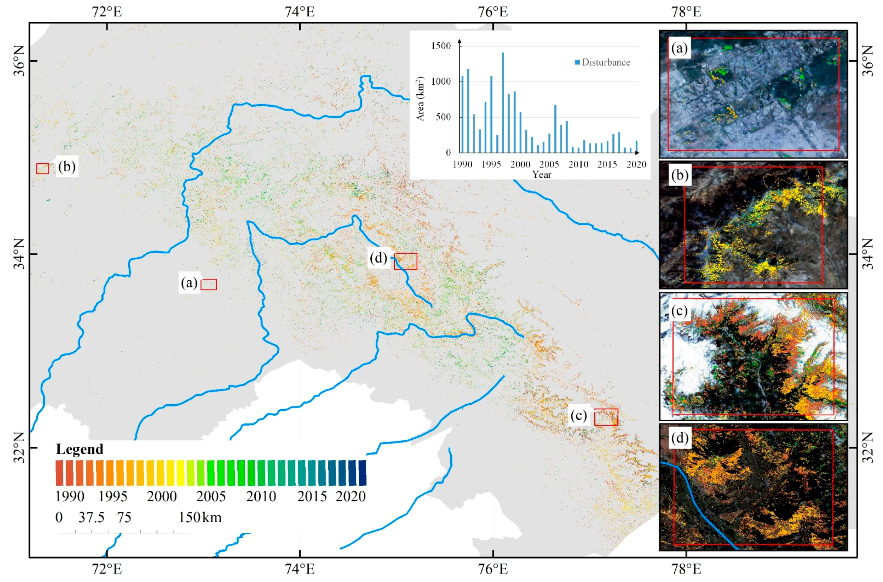
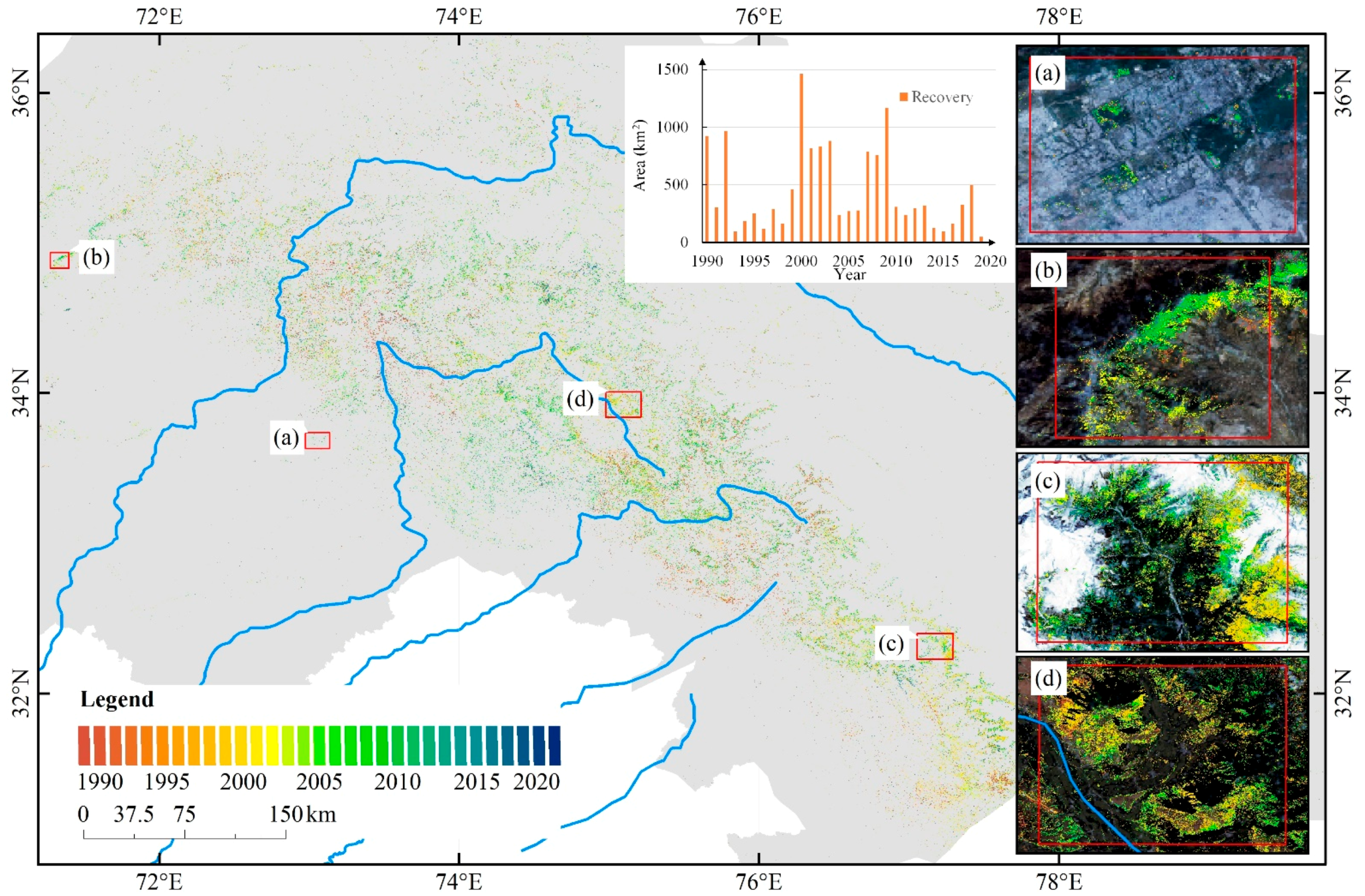
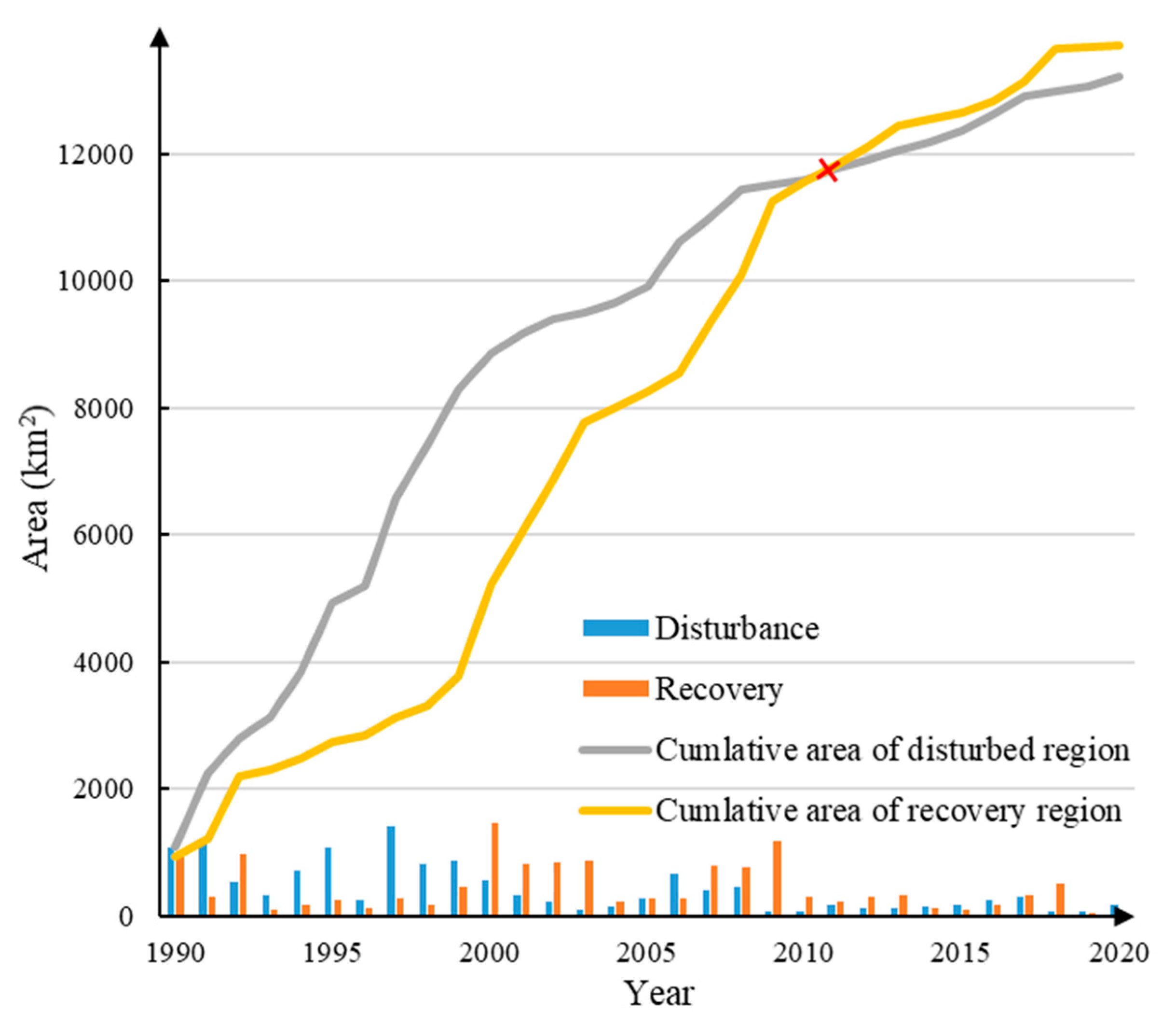
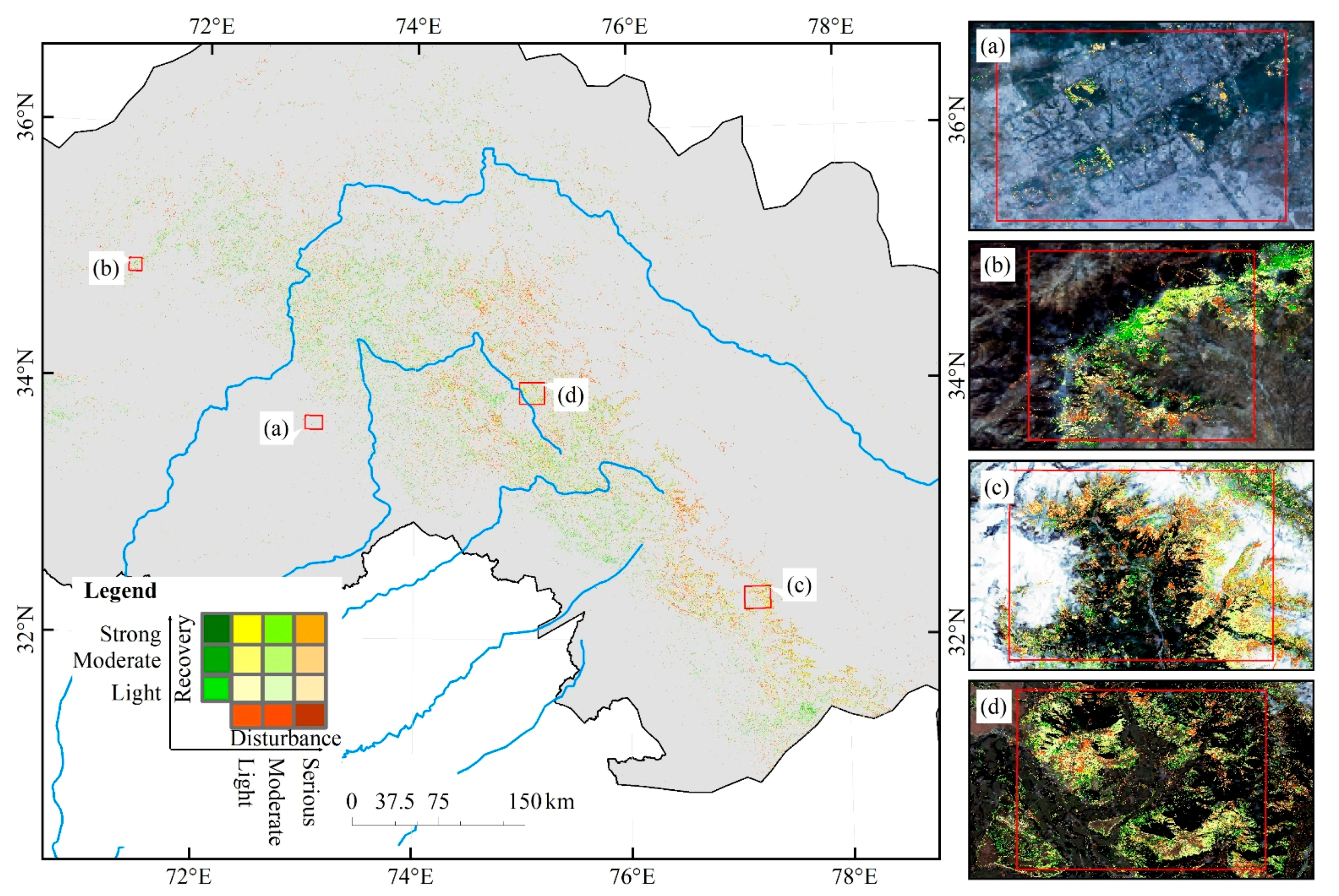
3.1. Spatial and Temporal Patterns of Forest Disturbance and Recovery

Figure 4 shows the spatial distribution of forest disturbances (including serious, moderate, and light disturbances) in the upper Indus Valley from 1990 to 2020 using transitional colors. Forest disturbances are widely distributed in the middle of the study area, mainly in the southwestern Himalayas and the southern Hindu Kush. Large areas of forest disturbance occurred in the upper reaches of the three rivers of Jhelum, Chenab, and Ravi and on both sides of the Kashmir Valley, largely distributed around cities and farmlands, between 1995 and 2015. In the past 31 years, a total of 13,233.55 km2 of forest was disturbed, accounting for 28.64% of the total forest area. The average disturbed area was 426.88 km2 per year, indicating that 0.92% of forests were disturbed at different levels per year on average. The annual disturbed area showed a fluctuating downward trend. In 1990, the disturbed forest area was 1080.17 km2, and reached a peak of 1410.23 km2 in 1997. After 2009, the disturbed forest area was less than 300 km2. The disturbance area from 1990 to 2001 accounted for 70% of the total disturbed area in 31 years, indicating that the disturbance mostly occurred in the first 10 years of the study period.
Figure 5 shows the spatiotemporal information of forest recovery (including strong, moderate, and light recovery) in the upper Indus Valley from 1990 to 2020, and the recovery area is widely distributed in the middle region as well as the disturbed area. Similar to the distribution of disturbances, the restored areas were also concentrated in the southwestern Himalayas and the southern Hindu Kush. In the past 31 years, a total of 13,702.55 km2 of forest was restored, accounting for 29.66% of the total forest area. The average annual recovery area was 442.01 km2, and 0.96% of the forests were restored on average. The annual recovery area showed a hump distribution trend. At the beginning, the recovery forest area was 924 km2 in 1990, and reached the peak of 1464.34 km2 in 2000. The area recovered from 1999 to 2010 accounted for 54.78% of the total area of 31 years, indicating that the forest recovery was mainly concentrated in the middle part of the study period.
From the results of the long-term analysis, it can be concluded that forest recovery and disturbance areas tend to be balanced in the upper Indus Valley. The recovery area was only 469 km2 larger than the disturbance area, accounting for 1.01% of the forest area in the upper Indus Valley. Figure 6 shows the interannual variation characteristics of disturbance and recovery. In 1990–2000, 70% of forest disturbance occurred, followed by 60% forest recovery in 1999–2012. In terms of spatial distribution, 70% of disturbances in 1990–2000 and 60% of recovery in 1999–2012 were mostly spatially coincident. This indicates that the disturbed forests from 1990 to 2000 were restored in the following 10 to 13 years, whether natural or man-made restorations. For the entire upper Indus Valley, 2012 is an important time node. The cumulative disturbance area since 1990 is equal to the cumulative recovery area this year, reaching a point of equilibrium. After 2012, the cumulative recovery area was slightly greater than the cumulative disturbance area.

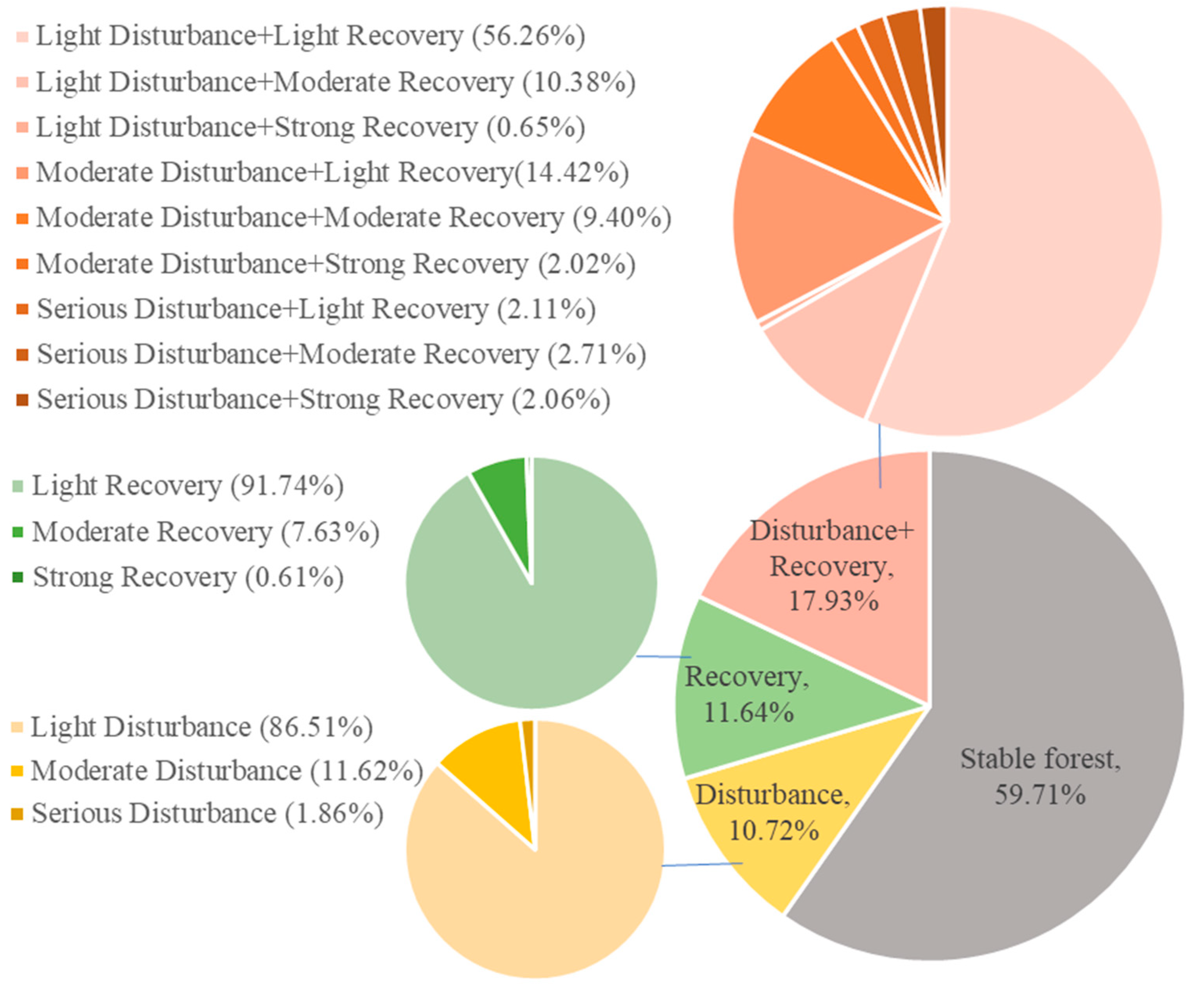
3.2. Temporal and Spatial Characteristics of Different Levels of Disturbance and Recovery

Figure 7 shows the spatiotemporal information distribution of 16 types of disturbance and recovery processes, including three different levels of combinations of disturbance and recovery. The results showed that 17.93% of the forests in the study area underwent two processes of disturbance and recovery from 1990 to 2020, especially in the areas bordering forests and farmland in the southern Himalayas and the sides of the Kashmir Valley.
Figure 8 shows the proportion of different combinations in the total forest area. A total of 59.71% of the forests remained stable in 31 years without disturbance or recovery. In the period from 1990 to 2020, forests that only underwent disturbances accounted for 10.72%, of which 86.51% were light, 11.62% were moderate, and only 1.86% were serious disturbances. The forests that only underwent recovery accounted for 11.64% of the total forest area, which was 0.92% more than the disturbance area. The results of different recovery level were as follows: light recovery (91.74%) > moderate recovery (7.63%) > strong recovery (0.61%).
The area where both disturbance and recovery occurred accounted for 17.93% of the total forest area, indicating that this part of the forest underwent a process of disturbance and recovery conversion. The areas of light disturbance and light recovery were the largest, accounting for 56.26%, followed by moderate disturbance + light recovery (14.42%), light disturbance + moderate recovery (10.38%), and moderate disturbance + moderate recovery (9.4%). The proportions of the other five combinations were all less than 3%. The results showed that forest disturbance and recovery in the study area were mainly light disturbances, and serious disturbances and strong recovery accounted for very few (<2%).
LandTrendr not only obtained spatiotemporal information of severely disturbed and obviously restored forest areas, but also captured the natural growth trend of forests or forest degradation caused by climate change and drought. Although there is no effective way to classify these areas in detail, obtaining varying degrees of disturbance and recovery is crucial for understanding the processes of forest change.

3.3. Accuracy Assessment of LandTrendr Results

The accuracy evaluation of the HGFC data and Google Earth images on LandTrendr segmentation results shows that the algorithm can effectively monitor forest disturbance and recover the footprint (Table 4). The different classes demonstrated high producer and user accuracies.
Analysis of the HGFC data showed that the highest user accuracy disturbance class was 91.69%, whereas the user accuracy for identifying both disturbance and recovery was 65.16%. There was a 26.15% confusion between the disturbance + recovery and disturbance classes, indicating that only one disturbance process was identified in the disturbance + recovery class. There was little difference among the three classes of producer accuracy: the highest accuracy of the recovery category was 87.22%, and the lowest accuracy of the disturbance category was 85.18%. In Google image-based evaluation, the highest user accuracy of 90.05% was achieved in the disturbance class (Table 5). In producer accuracy assessment, the highest accuracy was 91.84% for the disturbance class and the lowest was 61.86% for the recovery class.
The high producer and user accuracies of the disturbance and recovery categories indicate that the LandTrendr method is robust in obtaining disturbance and recovery footprint information.

4. Discussion

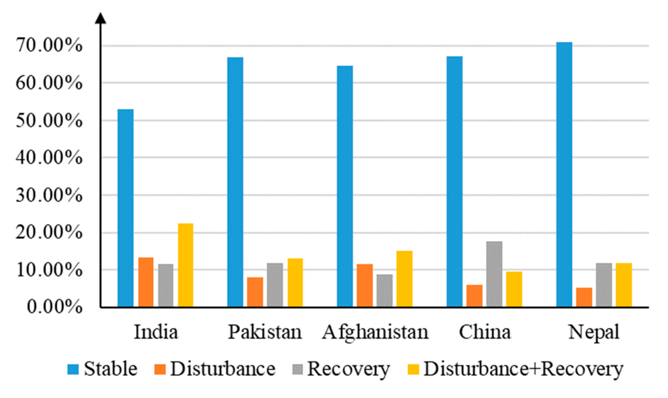
4.1. Forest Disturbance and Recovery in Different Regions

The results showed that, although the overall trend of forest disturbance and recovery was balanced, there were significant differences in forest disturbance and recovery in different regions due to the geographical environment and management policies. The forests in the upper Indus Valley are managed by five countries. To explore the changes in forests in different countries, we created statistics and analyzed results from the perspective of forest management.
Table 6 shows the area of stability, disturbance, recovery, and both disturbance and recovery have occurred in India, Pakistan, Afghanistan, China, and Nepal. The disturbed and recovered forests of the five countries showed significantly different characteristics. From 1990 to 2020, the forest stability in Nepal was the highest (71.03%), Pakistan and China had little difference (66.97% and 64.59%, respectively), and India had the least stability (52.98%). Figure 9 shows the proportion of disturbance and recovery areas in the forest area of the upper Indus Valley in different countries. The highest proportion of disturbance was 13.18% in India, and the least were 5.95% and 5.33% in China and Nepal, respectively. The area of forest recovery was highest in China (17.49%), followed by Pakistan (11.81%), Nepal (11.74%), India (11.41%), and Afghanistan (8.81%). In the region, where both disturbance and recovery have occurred, India accounted for the highest proportion at 22.42%, and Nepal for the lowest proportion at 11.89%.
Figure 10 shows the interannual variation characteristics of forest disturbance and recovery in the upper Indus Valley in different forest management regions. In India, the disturbance forest area has been larger than the recovery forest area for 31 years since 1990. By 2020, the disturbance and recovery forest area showed a trend towards balance, but there was still a 387.86 km2 gap. From 1990 to 1994, the accumulative recovery area of Afghanistan was larger than the accumulative recovery area. After 1994, the accumulative disturbance area continued to be larger than the accumulative recovery area. Although Afghanistan’s forest area in the upper Indus Valley is relatively small, the disturbance and recovery of forests did not reach equilibrium until 2020. There were two inflection points in the forest change trend in Pakistan. In 1993, the cumulative disturbance area in Pakistan exceeded the cumulative recovery area and lasted for 16 years. After reaching equilibrium in 2009, the forest change trend in Pakistan tended to recover. The interannual variation of forest in China and Nepal was similar, and the cumulative recovery area was always larger than the cumulative disturbance area after 1993. Many studies have pointed to forest disturbances in Nepal, but this study only focused on a very small portion of Nepal’s forests located in the upper Indus Valley, and the results represent only that portion of forests.

4.2. Analysis of the Causes of Disturbance and Recovery

There is a close relationship between the climate and vegetation in the Indus Valley. In the upper Sindh and Punjab, overgrazing and deforestation have led to the destruction of many natural vegetation types. In addition, humans have long interfered with natural water systems, and in Shivalik, deforestation has led to a marked deterioration of groundwater and vegetation cover. From 1990 to 2020, 59.71% of the forests in the upper Indus Valley remained stable, and the restored area was 0.92% greater than the disturbed area. Although the overall trend of forest change was balanced, there was still an imbalance among the five countries, especially in different provinces.
Table 7 shows the data of forest change in different administrative regions. Himachal Pradesh and Jammu and Kashmir are the two regions with the most disturbance area exceeding the recovery area, covering 362.77 km2 and 40.89 km2, respectively. Pathania et al. (2012) noted that the forest area in this region decreased with the passage of time, and grazing caused an obvious loss of plantation forest [42]. Other studies have shown that the large-scale introduction of horticultural cash crops in the region between 1998 and 2010 led to some significant changes in forest composition, with commercial cultivation leading to the decline of some important plant species [43]. We also observed that some reports indicate that the forest coverage in this area increased from 1991 to 2015, which can be explained by commercial tree planting [44]. Forest fires, landslides, and other natural disasters are also significant causes of forest disturbance in this region [45], but it is difficult to quantify the specific area of disturbance currently caused by these reasons. These regions should be aware that changes in the composition of forest species and ecological imbalances caused by deforestation and forest degradation may cause irreversible damage to unstable and fragile mountainous areas.
In the Gilgit Baltistan of Pakistan, the forest disturbance area was 40.89 km2 more than the recovery area, and the disturbance was mainly distributed in the Western border area with Afghanistan. Qamer et al. (2016) showed that the area was felled or severely degraded from 1990 to 2010 [18]. The results of this study and those of Qamer et al. (2016) show consistent temporal and spatial characteristics in the Gilgit Baltistan. The forests of Afghanistan are mainly distributed in the Eastern region, and the disturbance and recovery of the provinces are balanced, except in the Paktia, Paktika, and Nangarhar districts. A previous study on forest change in Northern Pakistan from 1990 to 2010 similarly showed that some assessment reports have grossly overstated deforestation rates, which is consistent with the findings of our study [18].
The main contribution of forest recovery came from the Khyber Pakhtunkhwa, Azad Kashmir, and Tibet, and the recovery areas were 537.05 km2, 168.89 km2, and 117.26 km2 more than the disturbance area, respectively. Forest recovery in the Khyber Pakhtunkhwa Province was primarily driven by the Khyber Pakhtunkhwa Billion Tree Forestation Project, which aims to plan, design, initiate, and implement the Green Growth Initiative in the forestry sector [46]. Khan et al. (2020) studied the temporal changes in forest cover, carbon storage, and corresponding CO2 emission/retention trends (1989–2018) in Azad Kashmir and showed that both forest cover and carbon storage increased significantly, and the research results were consistent with this study [47]. The Tibet Ali region, carried out from 2002 biological sand prevention engineering, implemented a five-phase afforestation project, which is consistent with the results of this study.

4.3. Method Limitations and Its Application

The LandTrendr spectral-temporal segmentation algorithm results may vary greatly according to different parameters and spectral indices [48]. The fixed parameters cannot obtain the optimal result, which needs to be further determined by combining the UI program provided by LandTrendr with real ground samples. For forest disturbance and recovery, the information extraction method used in this study can obtain spatiotemporal cognition of the forest change footprint in the upper Indus Valley. However, this approach does not distinguish between the possible causes of disturbance, such as deforestation, climate change, and geological hazards. The rate band in the results provided by LandTrendr provides a possible way to distinguish between these possible causes, which require further analysis.

5. Conclusions

To describe the disturbance and recovery of forests quantitatively and objectively in the upper Indus Valley, we used multi-source remote sensing data, the LandTrendr spectral-temporal segmentation algorithm, and a remote sensing big data computing platform to complete the monitoring of forest change footprint in the upper Indus Valley. The main conclusions are as follows:
(1) The LandTrendr algorithm combined with multi-source remote sensing data and the GEE big data platform completed forest change footprint tracking of forests in the upper Indus Valley for 31 years, and the algorithm showed stable robustness and portability.
(2) Forest disturbance and recovery were widespread in 1990–2020, most of the disturbance occurred in 1990–2000, the recovery was in 2000–2010, and equilibrium was widely attained in 2012.
(3) Forest disturbance and recovery in different forest management regions showed significant differences, and forest disturbance in India and Afghanistan did not reach equilibrium by 2020. Pakistan reached equilibrium in 2009, while Nepal and China showed relatively stable and continuous trends in forest recovery.
This study can further contribute to more effective forest management policy development by identifying the spatial and temporal patterns of disturbance and recovery for quantitative assessment.

Author Contributions

Conceptualization, methodology, and resources, X.Y. and J.W.; software, validation, data curation, and writing —original draft preparation, X.Y.; writing—review and editing, J.W. and X.Y. All authors have read and agreed to the published version of the manuscript.

Funding

Special acknowledgement should be expressed to the China–Pakistan Joint Research Center on Earth Sciences and the Construction Project of the China Knowledge Center for Engineering Sciences and Technology (Grant number CKCEST-2020-2-4), which supported the implementation of this study.

Institutional Review Board Statement

Not applicable.

Informed Consent Statement

Not applicable.

Data Availability Statement

The data presented in this study are available on request from the corresponding author.

Conflicts of Interest

The authors declare no conflict of interest.

References

  1. Bala, G.; Caldeira, K.; Wickett, M.; Phillips, T.J.; Lobell, D.B.; Delire, C.; Mirin, A. Combined climate and carbon-cycle effects of large-scale deforestation. Proc. Natl. Acad. Sci. USA 2007, 104, 6550–6555. [Google Scholar] [CrossRef] [PubMed] [Green Version]
  2. Bonan, G.B. Forests and climate change: Forcings, feedbacks, and the climate benefits of forests. Science 2008, 320, 1444–1449. [Google Scholar] [CrossRef] [PubMed] [Green Version]
  3. Mondal, P.; McDermid, S.S.; Qadir, A. A reporting framework for Sustainable Development Goal 15: Multi-scale monitoring of forest degradation using MODIS, Landsat and Sentinel data. Remote Sens. Environ. 2020, 237, 111592. [Google Scholar] [CrossRef]
  4. Attiwill, P.M. The disturbance of forest ecosystems—The ecological basis for conservative management. For. Ecol. Manag. 1994, 63, 247–300. [Google Scholar] [CrossRef]
  5. Seidl, R.; Fernandes, P.M.; Fonseca, T.F.; Gillet, F.; Jonsson, A.M.; Merganicova, K.; Netherer, S.; Arpaci, A.; Bontemps, J.D.; Bugmann, H.; et al. Modelling natural disturbances in forest ecosystems: A review. Ecol. Model. 2011, 222, 903–924. [Google Scholar] [CrossRef] [Green Version]
  6. Munoz, R.; Bongers, F.; Rozendaal, D.M.A.; Gonzalez, E.J.; Dupuy, J.M.; Meave, J.A. Autogenic regulation and resilience in tropical dry forest. J. Ecol. 2021, 109, 3295–3307. [Google Scholar] [CrossRef]
  7. Vina, A.; McConnell, W.J.; Yang, H.B.; Xu, Z.C.; Liu, J.G. Effects of conservation policy on China’s forest recovery. Sci. Adv. 2016, 2, 1500965. [Google Scholar] [CrossRef] [Green Version]
  8. Chen, Y.; Luo, G.; Maisupova, B.; Chen, X.; Mukanov, B.M.; Wu, M.; Mambetov, B.T.; Huang, J.; Li, C. Carbon budget from forest land use and management in Central Asia during 1961–2010. Agric. For. Meteorol. 2016, 221, 131–141. [Google Scholar] [CrossRef]
  9. Hansen, M.C.; Potapov, P.V.; Moore, R.; Hancher, M.; Turubanova, S.A.; Tyukavina, A.; Thau, D.; Stehman, S.V.; Goetz, S.J.; Loveland, T.R.; et al. High-resolution global maps of 21st-century forest cover change. Science 2013, 342, 850–853. [Google Scholar] [CrossRef] [Green Version]
  10. Immerzeel, W.W.; Lutz, A.F.; Andrade, M.; Bahl, A.; Biemans, H.; Bolch, T.; Hyde, S.; Brumby, S.; Davies, B.J.; Elmore, A.C.; et al. Importance and vulnerability of the world’s water towers. Nature 2020, 577, 364–369. [Google Scholar] [CrossRef]
  11. FAO. State of the World’s Forests 2011; Food and Agricultural Organization of the United Nations: Rome, Italy, 2011. [Google Scholar]
  12. Rashid, I.; Bhat, M.A.; Romshoo, S.A. Assessing changes in the above ground biomass and carbon stocks of Lidder valley, Kashmir Himalaya, India. Geocarto Int. 2017, 32, 717–734. [Google Scholar] [CrossRef]
  13. Zeb, A.; Hamann, A.; Armstrong, G.W.; Acuna-Castellanos, D. Identifying local actors of deforestation and forest degradation in the Kalasha valleys of Pakistan. For. Policy Econ. 2019, 104, 56–64. [Google Scholar] [CrossRef]
  14. Masek, J.G.; Huang, C.Q.; Wolfe, R.; Cohen, W.; Hall, F.; Kutler, J.; Nelson, P. North American forest disturbance mapped from a decadal Landsat record. Remote Sens. Environ. 2008, 112, 2914–2926. [Google Scholar] [CrossRef]
  15. Griffiths, P.; Kuemmerle, T.; Baumann, M.; Radeloff, V.C.; Abrudan, I.V.; Lieskovsky, J.; Munteanu, C.; Ostapowicz, K.; Hostert, P. Forest disturbances, forest recovery, and changes in forest types across the Carpathian ecoregion from 1985 to 2010 based on Landsat image composites. Remote Sens. Environ. 2014, 151, 72–88. [Google Scholar] [CrossRef]
  16. Pflugmacher, D.; Cohen, W.B.; Kennedy, R.E.; Yang, Z.Q. Using Landsat-derived disturbance and recovery history and lidar to map forest biomass dynamics. Remote Sens. Environ. 2014, 151, 124–137. [Google Scholar] [CrossRef]
  17. Joshi, A.K.; Joshi, P.K.; Chauhan, T.; Bairwa, B. Integrated approach for understanding spatio-temporal changes in forest resource distribution in the central Himalaya. J. For. Res. 2014, 25, 281–290. [Google Scholar] [CrossRef]
  18. Qamer, F.M.; Shehzad, K.; Abbas, S.; Murthy, M.S.R.; Xi, C.; Gilani, H.; Bajracharya, B. Mapping Deforestation and Forest Degradation Patterns in Western Himalaya, Pakistan. Remote Sens. 2016, 8, 385. [Google Scholar] [CrossRef] [Green Version]
  19. Gorelick, N.; Hancher, M.; Dixon, M.; Ilyushchenko, S.; Thau, D.; Moore, R. Google Earth Engine: Planetary-scale geospatial analysis for everyone. Remote Sens. Environ. 2017, 202, 18–27. [Google Scholar] [CrossRef]
  20. Huang, C.; Coward, S.N.; Masek, J.G.; Thomas, N.; Zhu, Z.; Vogelmann, J.E. An automated approach for reconstructing recent forest disturbance history using dense Landsat time series stacks. Remote Sens. Environ. 2010, 114, 183–198. [Google Scholar] [CrossRef]
  21. Verbesselt, J.; Hyndman, R.; Newnham, G.; Culvenor, D. Detecting trend and seasonal changes in satellite image time series. Remote Sens. Environ. 2010, 114, 106–115. [Google Scholar] [CrossRef]
  22. Hughes, M.J.; Kaylor, S.D.; Hayes, D.J. Patch-Based Forest Change Detection from Landsat Time Series. Forests 2017, 8, 166. [Google Scholar] [CrossRef]
  23. Deng, C.B.; Zhu, Z. Continuous subpixel monitoring of urban impervious surface using Landsat time series. Remote Sens. Environ. 2020, 238, 21. [Google Scholar] [CrossRef]
  24. Zhu, Z.; Zhang, J.; Yang, Z.; Aljaddani, A.H.; Cohen, W.B.; Qiu, S.; Zhou, C. Continuous monitoring of land disturbance based on Landsat time series. Remote Sens. Environ. 2020, 238, 11116. [Google Scholar] [CrossRef]
  25. Nature, W.W.F.f. As the World’s Population Grows, Forests Are Coming under More Pressure Than Ever. Available online: https://www.wwfpak.org/our_work_/forests/ (accessed on 18 December 2021).
  26. Roy, D.P.; Kovalskyy, V.; Zhang, H.K.; Vermote, E.F.; Yan, L.; Kumar, S.S.; Egorov, A. Characterization of Landsat-7 to Landsat-8 reflective wavelength and normalized difference vegetation index continuity. Remote Sens. Environ. 2016, 185, 57–70. [Google Scholar] [CrossRef] [Green Version]
  27. Zhu, Z.; Wang, S.; Woodcock, C.E. Improvement and expansion of the Fmask algorithm: Cloud, cloud shadow, and snow detection for Landsats 4–7, 8, and Sentinel 2 images. Remote Sens. Environ. 2015, 159, 269–277. [Google Scholar] [CrossRef]
  28. Zhu, Z.; Woodcock, C.E.; Olofsson, P. Continuous monitoring of forest disturbance using all available Landsat imagery. Remote Sens. Environ. 2012, 122, 75–91. [Google Scholar] [CrossRef]
  29. Yan, X.; Wang, J. Dynamic monitoring of urban built-up object expansion trajectories in Karachi, Pakistan with time series images and the LandTrendr algorithm. Sci. Rep. 2021, 11, 1–15. [Google Scholar] [CrossRef]
  30. Kennedy, R.E.; Yang, Z.G.; Cohen, W.B. Detecting trends in forest disturbance and recovery using yearly Landsat time series: 1. LandTrendr-Temporal segmentation algorithms. Remote Sens. Environ. 2010, 114, 2897–2910. [Google Scholar] [CrossRef]
  31. Kennedy, R.E.; Yang, Z.; Gorelick, N.; Braaten, J.; Cavalcante, L.; Cohen, W.B.; Healey, S. Implementation of the LandTrendr Algorithm on Google Earth Engine. Remote Sens. 2018, 10, 691. [Google Scholar] [CrossRef] [Green Version]
  32. Cohen, W.B.; Yang, Z.; Heale, S.P.; Kennedy, R.E.; Gorelic, N. A LandTrendr multispectral ensemble for forest disturbance detection. Remote Sens. Environ. 2018, 205, 131–140. [Google Scholar] [CrossRef]
  33. Lopez-Garcia, M.; Caselles, V. Mapping burns and natural reforestation using Thematic Mapper data. Geocarto Int. 1991, 6, 31–37. [Google Scholar] [CrossRef]
  34. Wilson, E.H.; Sader, S.A. Detection of forest harvest type using multiple dates of Landsat TM imagery. Remote Sens. Environ. 2002, 80, 385–396. [Google Scholar] [CrossRef]
  35. Tucker, C.J. red and photographic infrared linear combinations for monitoring vegetation. Remote Sens. Environ. 1979, 8, 127–150. [Google Scholar] [CrossRef] [Green Version]
  36. Salomonson, V.V.; Appel, I. Estimating fractional snow cover from MODIS using the normalized difference snow index. Remote Sens. Environ. 2004, 89, 351–360. [Google Scholar] [CrossRef]
  37. Huete, A.; Didan, K.; Miura, T.; Rodriguez, E.P.; Gao, X.; Ferreira, L.G. Overview of the radiometric and biophysical performance of the MODIS vegetation indices. Remote Sens. Environ. 2002, 83, 195–213. [Google Scholar] [CrossRef]
  38. Huang, C.; Wylie, B.; Yang, L.; Homer, C.; Zylstra, G. Derivation of a tasselled cap transformation based on Landsat 7 at-satellite reflectance. Int. J. Remote Sens. 2002, 23, 1741–1748. [Google Scholar] [CrossRef]
  39. Crist, E.P. A Tm Tasseled Cap Equivalent Transformation for Reflectance Factor Data. Remote Sens. Environ. 1985, 17, 301–306. [Google Scholar] [CrossRef]
  40. Baig, M.H.A.; Zhang, L.; Shuai, T.; Tong, Q. Derivation of a tasselled cap transformation based on Landsat 8 at-satellite reflectance. Remote Sens. Lett. 2014, 5, 423–431. [Google Scholar] [CrossRef]
  41. Liu, S.; Wei, X.; Li, D.; Lu, D. Examining Forest Disturbance and Recovery in the Subtropical Forest Region of Zhejiang Province Using Landsat Time-Series Data. Remote Sens. 2017, 9, 479. [Google Scholar] [CrossRef] [Green Version]
  42. Pathania, M.S.; Sharma, S.K. Impact of migratory animals on grazing lands: An evidence from Himachal Pradesh. Indian J. Anim. Res. 2012, 46, 40–45. [Google Scholar]
  43. Shah, S.; Sharma, D.P. Land use change detection in Solan Forest Division, Himachal Pradesh, India. Forest Ecosystems 2015, 2, 327–338. [Google Scholar] [CrossRef] [Green Version]
  44. Sharma, P.; Mahajan, A.; Lata, K.; Bharti, H.; Randhawa, S.S. An Analysis of the Temporal Changes in the Forests of Himachal Pradesh—A Review; State Centre on Climate Change State Council for Science: Shimla, India, 2015; Volume 10, pp. 63–76. [Google Scholar]
  45. Nandy, S.; Singh, C.; Das, K.K.; Kingma, N.C.; Kushwaha, S.P.S. Environmental vulnerability assessment of eco-development zone of Great Himalayan National Park, Himachal Pradesh, India. Ecol. Indic. 2015, 57, 182–195. [Google Scholar] [CrossRef]
  46. Khan, M.I.; Hussain, S.K.; Saad, H.; Rukh, G.; Ahmed, M.M.; Ahmad, I. Third Party Monitoring of Billion Trees Afforestation Project in Khyber Pakhtunkhwa Phase-Ii; World Wide Fund for Nature Pakistan (WWF-Pakistan): Lahore, Pakistan, 2017. [Google Scholar]
  47. Khan, I.A.; Khan, M.R.; Baig, M.H.A.; Hussain, Z.; Hameed, N.; Khan, J.A. Assessment of forest cover and carbon stock changes in sub-tropical pine forest of Azad Jammu & Kashmir (AJK), Pakistan using multi-temporal Landsat satellite data and field inventory. PLoS ONE 2020, 15, e0226341. [Google Scholar] [CrossRef] [Green Version]
  48. Hislop, S.; Jones, S.; Soto-Berelov, M.; Skidmore, A.; Haywood, A.; Nguyen, T.H. A fusion approach to forest disturbance mapping using time series ensemble techniques. Remote Sens. Environ. 2019, 221, 188–197. [Google Scholar] [CrossRef]
Figure 1. The study area is in the upper Valley of the Indus River. To highlight the forests, we used a Sentinel-2 image synthesized with false colors (the darker red represents the lusher vegetation).
Remotesensing 14 00744 g001
Figure 2. Flowchart of forest change footprint monitoring in the upper Indus Valley.
Remotesensing 14 00744 g002
Figure 3. LandTrendr pixel time-series segmentation. Image data were reduced to a single band or spectral index and then divided into a series of straight-line segments by breakpoint (red points) identification. For example, this figure shows the segmentation process of the NDVI, AB, and CD, which represent the steady state of the forest, where BC is fitted as a disturbance event, and CD is an inverse process of BC and is identified as a recovery process.
Remotesensing 14 00744 g003
Figure 4. Spatial and temporal footprint distribution map of forest disturbance. Four selected sub-areas in the figure represent disturbance result examples in different areas, including (a) plain area, (b) plain and alpine transition area, (c) alpine area, and (d) river valley area.
Remotesensing 14 00744 g004
Figure 5. Spatial and temporal footprint distribution map of forest recovery. Four selected sub-areas in the figure represent recovery result examples in different areas, including (a) plain area, (b) plain and alpine transition area, (c) alpine area, and (d) river valley area.
Remotesensing 14 00744 g005
Figure 6. Interannual variation characteristics of disturbance and recovery. The red cross represents the cumulative area of the disturbed region equal to the cumulative area of the recovery region in the upper Indus Valley.
Remotesensing 14 00744 g006
Figure 7. Spatial distribution of forest disturbance and recovery combinations with different levels. Four selected sub-areas in the figure represent different levels of disturbance and recovery examples in different areas, including (a) plain area, (b) plain and alpine transition area, (c) alpine area, and (d) river valley area.
Remotesensing 14 00744 g007
Figure 8. Proportion of disturbance and recovery of different levels in forest area.
Remotesensing 14 00744 g008
Figure 9. The proportion of forest disturbance and recovery area in the upper Indus Valley.
Remotesensing 14 00744 g009
Figure 10. Interannual variation characteristics of disturbance and recovery in in the upper Indus Valley. (a) India (b) Pakistan (c) Afghanistan (d) China (e) Nepal.
Remotesensing 14 00744 g010
Table 1. Datasets used in this study.
NameData SourceData Description
Landsat time-series remote sensing imageUSGS, filter and synthesize on GEEA total of 8203 remote sensing images were used, path and row as shown in Figure 1.
Google Earth imageGoogle Earth Pro SoftwareAssist in determining thresholds for different levels of disturbance and recovery; collect samples for accuracy assessment.
Hansen Global Forest Change datasets v1.8 (2000–2020) (HGFC) [9]University of MarylandResults from time-series analysis of Landsat images in characterizing global forest extent and change from 2000 through 2020. The data are used for an accuracy assessment.
Table 2. Bands/indices used in this study.
Band/Index NameDescriptionCalculate MethodReference
Blue, Green, Red, NIR, SWIR1, SWIR2Original bands from the TM, ETM+, and OLI.The SLC-off data were removed, and the harmonization function [26] was used for consistency processing along with ETM+ and OLI data to obtain the annual sequence images of six bands. /
Normalized burn ratio (NBR)Normalized difference indices generated by TM, ETM+, and OLI sensors.NBR = (NIR-SWIR2)/(NIR+SWIR2)[33]
Normalized difference moisture index (NDMI)Normalized difference indices generated by TM, ETM+, and OLI sensors.NDMI = (NIR-SWIR1)/(NIR+SWIR1)[34]
Normalized difference vegetation index (NDVI)Normalized difference indices generated by TM, ETM+, and OLI sensors.NDVI = (NIR-Red)/(NIR+Red)[35]
Normalized difference snow index (NDSI)Normalized difference indices generated by TM, ETM+, and OLI sensors.NDSI = (Green-SWIR1)/(Green+SWIR1)[36]
Enhanced vegetation index (EVI)A vegetation index calculated from three bands of TM, ETM+, and OLI sensors.EVI = 2.5 * ((NIR - Red)/(NIR + 6 * Red - 7.5 * Blue + 1))[37]
Tasseled cap brightness (TCB)It is derived from spectral data and the tasselled-cap transformation algorithm. The algorithm can compress spectral data into several bands of physical scene features with minimal information loss.TCB = 0.2043(Blue) + 0.4158(Green) + 0.5524(Red) + 0.5741(NIR) + 0.3124(SWIR1) + 0.2303(SWIR2)[38,39,40]
Tasseled cap greenness (TCG)TCG = −0.1603(Blue) − 0.2819(Green) − 0.4934(Red)) + 0.7940(NIR) − 0.0002(SWIR1) − 0.1446(SWIR2)
Tasseled cap wetness (TCW)TCW = 0.0315(Blue) + 0.2021(Green) + 0.3102(Red)) + 0.1594(NIR) − 0.6806(SWIR1) − 0.6109(SWIR2)
Tasseled cap wetness (TCA) TCA = arctan (TCB/TCG)
Table 3. Different levels of disturbance and recovery [41].
TypeLevelDescriptionThresholds
DisturbanceSeriousLand use type changes, deforestation, and forest fires caused complete changes in the surface; for example, the transition from forests to agricultural land and buildings.500 < magnitude
ModerateDue to different reasons such as selective logging, drought, or pests and diseases, the forest has been severely disturbed.350 < magnitude ≤ 500
LightLocal changes in the forest, forest disturbances can be reflected in high-resolution images, such as plenter-thinning in the management process. 200 < magnitude ≤ 350
RecoveryStrongThe transition from non-forest land use types to forest types is mainly through afforestation, and areas with better climate conditions can also be self-regulated or community succession through forest ecosystems.<−500
ModerateThe opposite process of moderate disturbance indicates the change of forest structure, such as the change from sparse forest to dense forest.−500 ≤magnitude < −350
LightDue to afforestation or self-recovery of forests, the density of forest structure gradually becomes higher, which can be observed in high-resolution images.−350 ≤magnitude < −200
Table 4. The accuracy assessment result was based on LandTrendr segmentation results and HGFC datasets.
Reference Data: HGFC Datasets (Pixels)
DisturbanceRecoveryDisturbance + RecoveryUser Accuracy
LandTrendr results (pixels)Disturbance72655936591.69%
Recovery101446172981.57%
Disturbance + Recovery2508362365.16%
Producer accuracy85.18%87.22%86.88%
Overall accuracy86.01%
Kappa0.73
Table 5. The accuracy assessment result was based on LandTrendr segmentation results and samples from Google Earth images.
Reference Data: Google Earth Images (Pixels)
DisturbanceRecoveryDisturbance + RecoveryUser Accuracy
LandTrendr results (pixels)Disturbance15201076190.05%
Recovery356333689.91%
Disturbance + Recovery10010283780.56%
Producer accuracy91.84%61.86%89.61%
Overall accuracy87.17%
Kappa0.79
Table 6. Forest disturbance and recovery statistics in the upper Indus Valley (unit: km2).
RegionForest AreaStableDisturbanceRecoveryDisturbance + Recovery
India23,345.8112,368.8 (52.98%)3078.08 (13.18%)2664.1 (11.41%)5234.9 (22.42%)
Pakistan20,366.9613,640.44 (66.97%)1646.3 (8.08%)2405.44 (11.81%)2678.15 (13.15%)
Afghanistan1463.67945.44 (64.59%)167.42 (11.44%)128.88 (8.81%)221.41 (15.13%)
China1009.24626.36 (62.06%)60.09 (5.95%)176.51 (17.49%)146.25 (14.49%)
Nepal6.574.67 (71.03%)0.35 (5.33%)0.77 (11.74%)0.78 (11.89%)
Disturbance + Recovery means both disturbance and recovery have occurred
Table 7. Forest disturbance and recovery area of 28 administrative regions in the upper Indus Valley (km2).
Forest Management CountryProvinceForest AreaStableDisturbanceRecoveryRecovery − Disturbance
AfghanistanBamian0.320.210.100.07−0.02
Badakhshan10.107.431.532.210.68
Baghlan17.4811.754.913.53−1.38
Ghazni0.170.060.100.07−0.02
Kabol4.892.311.192.211.02
Kapisa59.4941.0212.2213.120.90
Konarha920.04627.05212.51209.93−2.58
Laghman132.28100.7021.8620.38−1.47
Lowgar8.224.531.763.201.44
Nangarhar102.2456.9234.7027.47−7.23
Paktia124.1550.6364.7643.06−21.70
Paktika22.676.4915.087.61−7.47
Parvan42.8226.5111.6311.29−0.34
Takhar0.010.010.000.000.00
Vardak18.7910.086.696.32−0.37
ChinaXinjiang9.186.102.601.76−0.84
Xizang1000.05620.26203.74321.00117.26
IndiaHimachal Pradesh8259.543997.953423.463060.69−362.77
Haryana0.100.030.060.060.00
Jammu and Kashmir14,960.138318.084831.744784.82−46.92
Punjab11.704.834.245.871.63
Uttar Pradesh114.3447.7153.4347.49−5.93
NepalKarnali6.574.671.131.550.42
PakistanAzad Kashmir4517.453036.43948.271117.16168.89
Federally Administered Tribal Areas 1017.79734.91160.99234.3473.35
Gilgit Baltistan 4248.702689.321126.951086.06−40.89
Khyber Pakhtunkhwa10,073.756802.692002.932539.98537.05
Punjab 509.27374.6984.74105.2120.47
Total 46,192.2627,583.364952.125375.30423.18
Publisher’s Note: MDPI stays neutral with regard to jurisdictional claims in published maps and institutional affiliations.

