Article

A Combined Approach for Retrieving Bathymetry from Aerial Stereo RGB Imagery

1
College of Information, Shanghai Ocean University, 999 Hucheng Huanlu Road, Shanghai 201308, China
2
College of Marine Science, Shanghai Ocean University, 999 Hucheng Huanlu Road, Shanghai 201308, China
*
Author to whom correspondence should be addressed.
Remote Sens. 2022, 14(3), 760; https://doi.org/10.3390/rs14030760
Submission received: 27 December 2021 / Revised: 1 February 2022 / Accepted: 2 February 2022 / Published: 7 February 2022
(This article belongs to the Section Ocean Remote Sensing)

Abstract

:
Shallow water bathymetry is critical in understanding and managing marine ecosystems. Bathymetric inversion models using airborne/satellite multispectral data are an efficient way to retrieve shallow bathymetry due to the affordable cost of airborne/satellite images and less field work required. With the increasing availability and popularity of unmanned aerial vehicle (UAV) imagery, this paper explores a new approach to obtain bathymetry using UAV visual-band (RGB) images. A combined approach is therefore proposed for retrieving bathymetry from aerial stereo RGB imagery, which is the combination of a new stereo triangulation method (an improved projection image based two-medium stereo triangulation method) and spectral inversion models. In general, the inversion models require some bathymetry reference points, which are not always feasible in many scenarios, and the proposed approach employs a new stereo triangulation method to obtain reliable bathymetric points, which act as the reference points of the inversion models. Using various numbers of triangulation points as the reference points together with a Geographical Weighted Regression (GWR) model, a series of experiments were conducted using UAV RGB images of a small island, and the results were validated against LiDAR points. The promising results indicate that the proposed approach is an efficient technique for shallow water bathymetry retrieval, and together with UAV platforms, it could be deployed easily to conduct a broad range of applications within marine environments.

1. Introduction

Shallow water regions’ bathymetry is important in various managements and modelling, such as navigation and transportation [1], modelling of sediment deformation [2], coastal line or water bank erosion [3,4], and the needs of sand mining and beach nourishment [5]. Bathymetry retrieval techniques can be sorted into two broad categories according to the principals that are used: geometric measurements and radiometric measurements. Geometric methods are based on the signal/ray travel return time to calculate the distance or using two or multiple optical rays to triangulate the depths; these methods include traditional echo sounding [6], two-medium photogrammetric triangulation [7,8], LiDAR [9], and so on. Radiometric methods (refer as satellite-derived bathymetry (SDB) methods) [10,11,12,13] are based on radiative transfer, where atmosphere composition and water column, as well as seabed type and composition, will affect the spectral information acquired using multispectral/hyperspectral imaging sensors. SDB methods usually use inversion models to infer the depth information. Some popular methods are introduced in the next section and a new combined approach for bathymetry retrieval is proposed in Section 3.

2. Bathymetric Retrieval Methods Review

On the category of geometric measurements to obtain bathymetry, echo sounding techniques are employed for deep water measurement but are usually not suitable for shallow water due to the vessel’s access. Airborne LiDAR becomes a promising technique to efficiently obtain shallow bathymetry; its accuracy is very high but very expensive to employ. With the rapid development of UAV technologies, imaging model-based methods [14] to obtain the bathymetry have become a popular choice for shallow bathymetry retrieval compared to sound-based methods or LiDAR. Imaging model-based correction requires rigorous mathematic equations through collinearity and Snell’s law, and it is difficult to implement due to the rigorous requirements and complexity [14,15].
To improve the accuracy of bathymetry acquisition by imaging model-based methods, Partama et al. [16] proposed an empirical method to correct the refraction effect by using the procedures of Structure-from-Motion (SfM) and Multi-View Stereo (MVS). Their method utilizes the empirical relationship between the measured true depth and estimates apparent depth to generate an empirical depth correction factor. Mandlburger et al. [17] proposed deriving bathymetry using RGBC (red, green, blue, costal blue) aerial images and a deep neural network method, and laser point clouds serve as the reference data and training data for the method. Murase et al. [18] proposed an approximation method to solve the position problem through the incident angles of light rays from an underwater object to two cameras. They mentioned that the horizontal shift can be neglected when the interest point is not on the vertical bisector of the shooting positions. Shan [19] suggested that a two-medium refraction problem can be described as a radial component or equivalent to correct the camera focal length. Skarlatos and Agraflotis et al. [20] proposed a non-iterative method based on machine learning to re-project an original image to an image that does not have any refraction effects, and then employed SfM and MVS techniques to obtain bathymetry. Cao et al. [15] proposed an algorithm to obtain the optimal observation position when the conjugate light rays were not intersecting. Although the abovementioned methods can improve the accuracy of water depth to a certain degree, the positions of observation points must be taken into account; otherwise, they will introduce new errors.
Another category of bathymetry techniques is based on radiometric measurements–SDB. SDB methods use the Beer–Lambert Law (in this case wavelength-dependent exponential attenuation of light in the water column) to derive inversion models. Assuming some references are available for estimating inversion models’ coefficients, it is generally possible to inverse a large area’s bathymetry using the models and estimated coefficients. There are 4 classic global inversion models: single-band bathymetric inversion model [10], two-band bathymetric inversion model [21], multi-band bathymetric inversion [22] model, and artificial neural network (ANN) method to inverse bathymetric [23].

3. A Proposed Combined Approach for Bathymetry Retrieval

In order to avoid the computational complexity of imaging model-based correction, a projection image based two-medium stereo triangulation method (hereinafter referred to as ST method) is proposed to make the water depth calculation simpler. The projection image concept was first introduced by one of the authors of [24], and utilizing the projection image, [24] achieves elevation correction of a single target point on the ground and refinement of the building edges. In this paper, this work was extended to take into account the ray refraction through two-medium photogrammetry, and the resultant projection images are then well suitable for quick and simple water depth triangulation. The ST method served as the water depth reference provider for inversion methods. The Geographical Weighted Regression (GWR) model, which has a character of weighting distribution, was used during the inversion model’s regression. In order to obtain the effective variables of the GWR model, we use principle component analysis (PCA) to extract the optimal component information from a set of combinations of RGB band ratios. Legleiter [11] proposed that the natural logarithmic values of the band ratios can be regarded as the appropriate estimators of water depths; therefore, the natural logarithmic value of the optimal RGB band ratio was used as the model’s estimator to estimate the model’s coefficients.
The details of the projection image based two-medium stereo triangulation method and GWR model are described in Section 3.1 and Section 3.2, respectively. The efficiency of the combined approach is illustrated by a bathymetry inversion experiment in Section 4.1. In Section 4.2, different numbers of triangulation points are used as reference points of the GWR model for inverse bathymetry of an island’s surrounding area, using the relative experiments to validate the superiorities of the combined approach. Furthermore, the inversion results of the GWR model are compared with that inversed by the MLR model.

3.1. The Projection Image Based Two-Medium Stereo Triangulation Method

The ST method is the extended version of the method used for elevation correction and refinement [24]. Similar to orthoimage generation process (forward and backward projections) [25], a projection image is obtained by projecting the original image onto a horizontal plane that has a constant elevation. It can be proven that in the two-medium photogrammetry case, although the ray refracts when passing through the air-water interface, all the projected points of an underwater vertical line still form a straight locus either on the left or right projection image. Therefore the same projection image method used in [24] can be applied to correct and refine the water depths of underwater points.
The relationships of underwater points (P, P1, and P2), projection points (PL, PR, PL1, PL2, PR1, and PR2), camera centers (SL and SR), and projected camera centers (SL’ and SR’) are shown in Figure 1. Through searching along the vertical line passing through P, all the projected points of the line can be mapped onto a locus LL (on the left projection image) or LR (on the right projection image). Assuming the searching is performed between points P1 and P2 (P is located somewhere on the line segment between P1 and P2), PL, PR, PL1, PL2, PR1, and PR2 are the projected points of P, P1, and P2 (L mean on the left projection image and R means on the right projection image), respectively. The depth (ZP) of P can be determined by comparing the correlation coefficients of the left and right candidate pairs (PL and PR; PL1 and PR1; PL2 and PR2).
There are three major advantages or special properties of projection images that make the projection image concept very attractive, especially from the computation efficiency aspect:
  • All projection images are within the same spatial coordinate system;
  • All projection images’ pixels have the same ground sample distance (GSD) and are not affected by any rotation angles because the rotation angles are zeros; and
  • When the elevation of target point is equal to the horizontal plane elevation Z0, the projected points of the target point on the left and right projection images share the same position.
When the original image is projected to an air-water interface with elevation Z0, the projected point P (XP, YP, Z0) can be obtained by Equation (1):
{ X P = ( a 1 ( x x 0 ) + a 2 ( y y 0 ) a 3 f c 1 ( x x 0 ) + c 2 ( y y 0 ) c 3 f ) ( Z 0 Z S ) + X S Y P = ( b 1 ( x x 0 ) + b 2 ( y y 0 ) b 3 f c 1 ( x x 0 ) + c 2 ( y y 0 ) c 3 f ) ( Z 0 Z S ) + Y S
where x, y are the original image coordinates; x0, y0 are the camera’s principal points and f is the camera’s focal length; (XS, YS, ZS) are the coordinate of camera projection center S; (ai, bi, ci) (i = 1, 2, 3) denote the nine parameters of the rotation matrix of the original image [26].
In the two-medium photogrammetry case, rigorous geometry is taken in account in the proposed method. According to Snell’s Law, the relationship of a left projected point PL (XPL, YPL, Z0) and the searching point Pi (XP, YP, ZPi) can be expressed in Equation (2):
{ n 2 = sin 2 α L sin 2 β L = ( X P L X S ) 2 [ ( X P X P L ) 2 + ( Z 0 Z P i ) 2 ] ( X P X S ) 2 [ ( X P L X S ) 2 + ( Z P i Z 0 ) 2 ] n 2 = sin 2 α L sin 2 β L = ( Y P L Y S ) 2 [ ( Y P Y P L ) 2 + ( Z 0 Z P i ) 2 ] ( Y P X P L ) 2 [ ( Y P L Y S ) 2 + ( Z P i Z 0 ) 2 ]
where n is the ratio of water refractive index and air refractive index, αL is the angle of incidence to the left projection image, and βL is the angle of light refraction at the left projection image.
Utilizing Equation (2), a series of candidate pairs (left and right projected points) of an underwater point can be obtained. Using a simple matching technique (cross correlation coefficients) the best candidate pair can be found for the underwater point. The cross correlation coefficients can be computed by the normalized cross correlation coefficient (NCC) [27,28] image matching technique:
N C C i ( P Li , P Ri ) = s W ( I L i ( s L i ) I L i ¯ ) ( I R i ( s R i ) I R i ¯ ) s W ( I L i ( s L i ) I L i ¯ ) 2 s W ( I R i ( s R i ) I R i ¯ ) 2
I L i ¯ = 1 m × n s W I L i ( s L i )                 I R i ¯ = 1 m × n s W I R i ( s R i )               i = 1 , 2 , 3 , , n
where ILi, IRi denote the image intensity values of the points PLi, PRi on their projection images within a correlation window W. m and n are window W’s size, and sLi, sRi are the pixels in window W on the left and right projection images, respectively. The NCCi value mainly depends on ILi and IRi, which are defined by the pixel values sLi and sRi.
Using the projection images, the steps of the ST method to obtain a target point’s water depth are described as follows:
  • Projecting the original images to the air-water interface to generate projection images;
  • Locating the target point’s horizontal position (X, Y), obtaining a series of depth candidates for the target point within the reasonable water depth range (hmin, hmax) and depth searching increment (k), and choosing an appropriate cross correlation window size (m × n);
  • Computing the candidate pairs of searching points using Equation (2);
  • Computing the correlation coefficients of the candidate pairs by Equation (3); and
  • Finding the pair with the maximum correlation coefficient and regarding its corresponding depth as the optimal depth position of the target point.

3.2. Geographically Weighted Regression (GWR) Model

The GWR model has many applications by the spatial heterogeneous relationship in the inversion process, such as housing market modelling [29], urban analysis [30], ecology and environmental science [31], and infectious disease epidemiology [32]. The GWR model was employed by Kim [33] for bathymetry inversion model’s regression and their experiments indicate that better results can be obtained using the GWR model compared to the multiple linear regression (MLR) model and artificial neural network (ANN) model.
Compared to global regression models, such as the MLR model or ANN model, the GWR model reflects the spatially varying relationships, and the coefficients are the functions of special locations [34]. The GWR model can be described using Equation (4):
y i = β 0 ( u i , v i ) + k = 1 m β k ( u i , v i ) x i k + ε i               i = 1 ,   2 ,   ,   n
where yi is the estimated water depth of sample i; xik is the kth explanatory variable of sample i; m is the number of explanatory variables; β0 is the intercept parameter of sample i; βk is the local regression coefficient for the kth explanatory variable of sample i; εi is the random error of sample i; (ui, vi) is the position coordinate of sample i.
The set of coefficients varies continuously by the location changes over the experimental area in the GWR model, where the regression point that is nearer to the observation point has more influence in the set of coefficients than a point farther away [35]. The set of regression coefficients around the reversion point at the location (ui, vi) can be estimated by weight least squares [36]. The key to regression coefficients is selecting the weighting function and kernel function. Considering that a lot of the observations in this study are clustered distribution around the experimental area, adaptive kernel was chosen to provide the geographic weighting in GWR [28], and the Akaike Information Criterion (AIC) [37] bandwidth method was used to compute the bandwidth to control the size of the kernel.

3.3. Bathymetric Accuracy Assessment Criteria

To evaluate the performance of ST method and the combined approach, mean absolute error (MAE), root mean squared error (RMSE), and coefficient of determination (R2) are chosen as the criteria to assess the bathymetric accuracy, where R2 varies from 0 to 1, and the value closer to 1 denotes the better model performance. The corresponding equations are expressed as Equations (5)–(7):
MAE = 1 n i = 1 n | Z i H i |
RMSE = i = 1 n ( Z i H i ) 2 n
R 2 = 1 i = 1 n ( Z i H i ) 2 i = 1 n ( Z i Z ¯ ) 2
where Zi and Hi denote the real water depth and estimated depth of the test point i respectively, Z ¯ denotes the mean value of n real water depths, and n is the number of test points.

4. The Experiments of Retrieving Bathymetry Using the Combined Approach

To verify the proposed combined approach, a bathymetry retrieval experiment in the surrounding region of an island (18°39′N, 110°17′E) was conducted. The shallow water around the island is very clear and the visibility can reach to 10 m in depth. The total 50 images with more than 0.75 overlap rates were captured using a Phantom4 RTK camera mounted on a small lightweight UAV. The UAV flying height was around 250 m above the water level. The image size was 5472 × 3648 pixels, the pixel size was 2.41 × 2.41 μm2, and the focal length was 9 mm. A total of 32 ground control points (the black triangles in Figure 2) sampled from LiDAR points, of which the accuracies were 0.1 m, 0.1 m, 0.2 m in X, Y, Z directions, respectively, were used for image calibration and orientation. An iterative camera calibration method was used [38] to estimate the camera lens distortion. The distortion residuals of the calibrated images reported less than 0.58 pixels, and the image orientation accuracies after the block adjustment applied were around 0.25 m, 0.24 m, and 0.55 m in X, Y, and Z directions, respectively. The elevation of air-water interface was determined manually using the air-water interface points through the forward stereo triangulation method [25]. The projection images were then generated by projecting the original images onto the air-water interface plane. Figure 2 shows the mosaic image composed using 5 projection images. There are slight displacements among the projected images, mainly because the region shares different elevations with the air-water interface plane.
Besides UAV RGB images, the LiDAR point cloud data of the experimental area were also acquired from an UAV-borne photon-counting bathymetric Lidar. This instrument uses the time-of-flight distance measurement principle of infrared nanosecond pulses for topographic applications and green (532 nm) nanosecond pulses for bathymetric applications. Figure 3 shows the bathymetry with 1 m spatial resolutions derived by interpolating those LiDAR points using the ordinary kriging method [39]. The interpolated bathymetry was used as the evaluation and validation data to compare and validate the combined approach.

4.1. Bathymetry Determination Using the Combined Approach

Following the ST method’s steps described in Section 3.1, 520 underwater points (shown as yellow points in Figure 2) were triangulated to obtain water depths, and the method was achieved in the environment of VC++ 2013. These 520 points were mainly distributed in the test area within 15 m of water depth. The triangulated depths are compared with the depths of their nearest LiDAR points’. When applying the ST method, considering that the water depths of 520 points are less than 15 m, the hmin was set to 0 m and the hmax was set to 15 m. The cross correlation window size had a strong influence on the results [40]; a 51 × 51 window size was set as cross correlation window size and 0.2 m as the depth searching interval—the same as the projection image’s resolution. A series of candidate pairs and their corresponding correlation coefficients were obtained based on the above setting parameters. The optimal depth position of the target point, therefore, can be determined using the maximum correlation coefficient criterion, for example. All 520 points were tested by ST method, and 400 points out of 520 points that had maximum coefficients greater than 0.6 were chosen as the acceptable points. Those 400 points were then compared with their nearest LiDAR points, shown in the corresponding scatter diagram in Figure 4a, and MAE reached 1.595 m and RMSE reached 1.843 m. The large residuals can be attributed to the fact that the ST method ignores the sea surface undulations due to waves and refractions’ change, as well as some test points with weak textures.
In order to infer the bathymetry of the experimental area, the obtained triangulation depths were used as the reference depths of the inversion model. Then the GWR model (introduced in Section 3.2) was used as inversion model to infer bathymetry of the experimental area, and PCA was used to extract the optimal band ratio that can reveal the most information among the 6 band ratios (DNR/DNG, DNR/DNB, DNG/DNR, DNG/DNB, DNB/DNR, and DNB/DNG) in the RGB image. As the result of PCA, the ratio of the digital number red band (DNR) and digital number green band (DNG) had the highest component score, which explained 92.1% of the total band ratios’ information. Then the natural logarithmic values (ln(DNR/DNG)) of the DNR and DNG ratios were used as the variables of GWR model. Here, the obtained 400 triangulation depths were used as the reference depths of the GWR model and their corresponding ln(DNR/DNG) values were used as the model’s variables to estimate the model’s parameters. Then 400 reference depths can be calibrated by the model’s parameters. Figure 4b shows the scatter diagram of 400 calibrated values when comparing with the corresponding 400 LiDAR depths, and MAE and RMSE are 1.050 m and 1.383 m, respectively.
From the inversion results, the precisions of reference points have improved after being calibrated by the model’s parameters. This indicates that the combined method, which utilizes the GWR model combined with the ST method to obtain bathymetry, is an effective way, and this method is easy to implement since only RGB images are required.

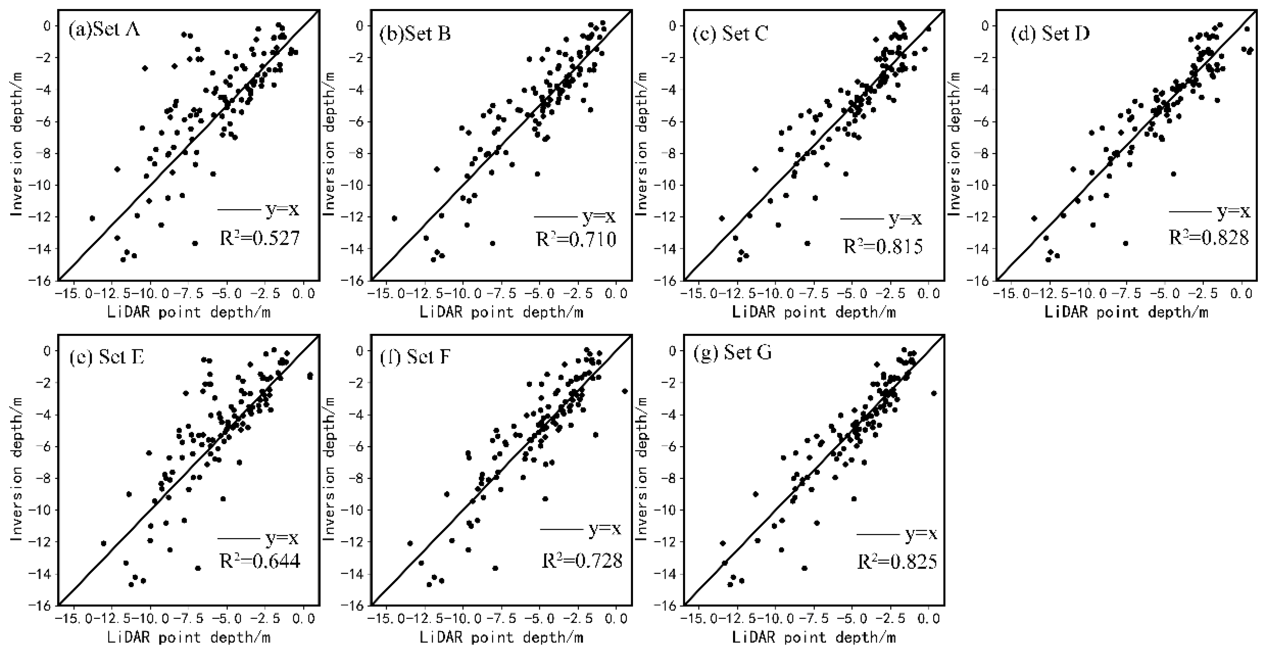
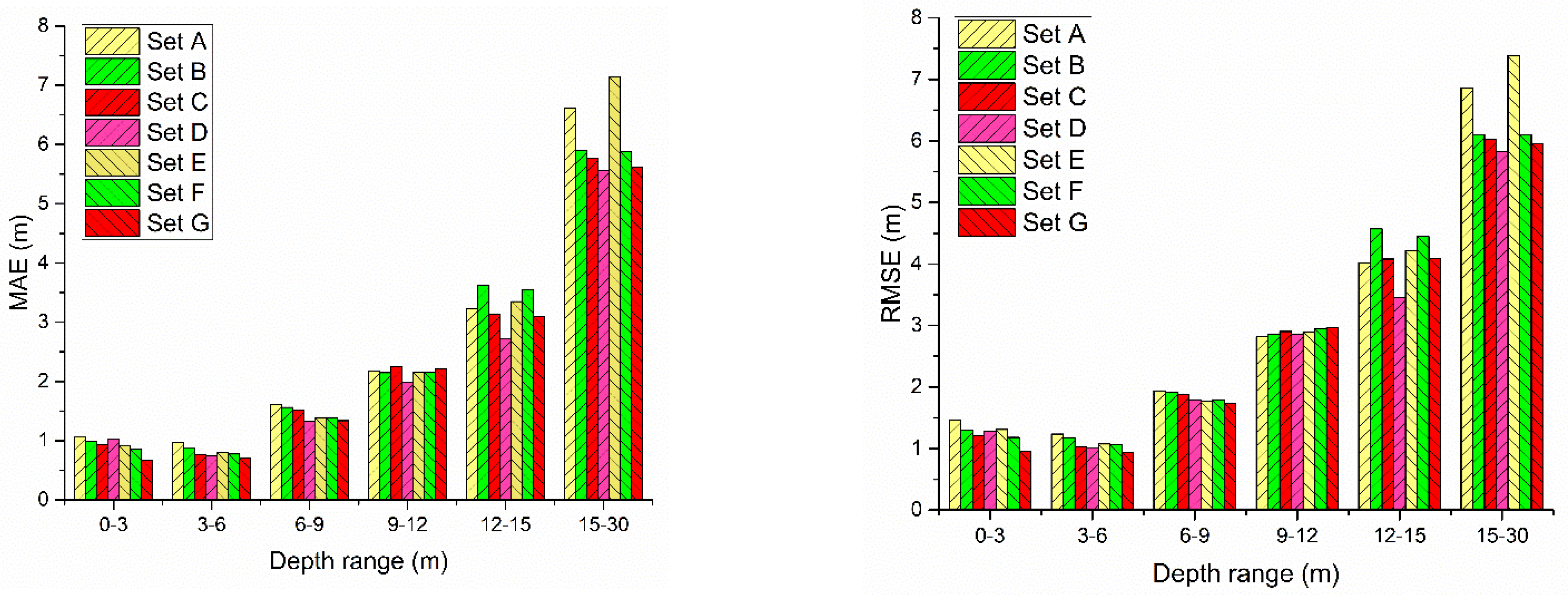
4.2. Evaluation of the Combined Approach

Section 4.1 validates that the GWR model combined with depths obtained by the ST method is an effective way to inverse bathymetry. To further illustrate the advantages of the combined approach, the inversion results retrieved by the combined method are compared with that inferred by the GWR model combined with LiDAR points. Considering the general situation, the number of water depth points is limited because the depths are usually acquired from electronic charts, LiDAR data, or field depths measurement with bathymetric instruments, and these technologies are difficult to carry out. Four triangulation sets (Set A, Set B, Set C, and Set D) of triangulation depths as reference points for the GWR model were carried out. The reference points (120 points, 200 points, 300 points, and 400 points) of the 4 sets were derived from 400 triangulation points, which were obtained by the ST method. Table 1 shows the MAE and RMSE of the reference points of the 4 triangulation sets when compared with their nearest LiDAR points, and Figure 5 shows the positions of reference points in 4 triangulation sets. Similarly, another 3 LiDAR sets (Set E, Set F, and Set G) experiments, which took LiDAR points as reference points of the GWR model, were tested. The LiDAR points were the nearest points of reference in Set A, Set B, and Set C. Besides these points being used as reference points in inversion, 120 LiDAR points were independently selected (Figure 5) as validation points to validate the inversion results obtained by the 4 triangulation sets or 3 LiDAR sets, respectively. Table 2 shows the comparison results of 120 validation points and their corresponding estimation values acquired by 4 triangulation sets and 3 LiDAR sets, and Figure 6 shows the scatter plots of 120 estimation values derived from 4 triangulation sets and 3 LiDAR sets when compared with their LiDAR depths.
From Table 1 and Table 2, the accuracies of 120 validation points in 4 triangulation sets increase with an increase of the number of reference points, although the accuracies of the reference points decrease. This phenomenon illustrates that in the case of low precision of reference points, using more reference points can also obtain high precision inversion results. Similarly, by comparing the inversion results of 4 triangulation sets and 3 LiDAR sets, the phenomenon is also proven. Using the ST method to obtain depth is a cost-effective approach, and it has the characteristics of semi-automation and fast acquisition of a large number of points’ depth. Combining the method with the GWR model is a high-efficiency way to inverse bathymetry, since only UAV RGB images are required. Additionally, from comparing the inversion results with the high-precision LiDAR points in Table 2 and Figure 6, the combined approach is also proven to have high inversion precision.
According to the GWR model and its reference points, the local regression coefficients and intercept parameters corresponding to 1 m spatial resolutions of the experimental area were estimated, and then the experimental area’s bathymetry with 1 m spatial resolutions could be derived by the corresponding local regression coefficients and intercept parameters. In order to further validate the combined approach, the absolute residuals between the interpolation bathymetry (Figure 3) of dense LiDAR points and the inferred bathymetries by 4 triangulation sets and 3 LiDAR sets are showin in Figure 7. Table 3 shows MAE and RMSE in the whole experimental area by per-pixel comparison between the interpolation bathymetry and the inferred bathymetries of 4 triangulation sets and 3 LiDAR sets.
As shown in Figure 7 and Table 3, bathymetry obtained in Set D is closest to interpolation bathymetry. This phenomenon indicates that the triangulation depths can be used to inverse bathymetry, and that abundant triangulation depths involved in inversing the bathymetry can get better results than those inversed by limited number measured depths such as LiDAR depths. The bigger residuals are usually found in the area that has a depth of more than 12 m; this phenomenon can be attributed to the fact that the reference points are mainly distributed within 12 m depth areas.
To better analyze the errors of different depths on the bathymetries retrieved by 4 triangulation sets and 3 LiDAR sets, the experimental regional depths were divided into 6 depth ranges, and each depth range and its corresponding MAE and RMSE are shown in Figure 8. As Figure 8 shows, the inversion precision has increased in the depth of the 3–30 m range by increasing the number of reference points. For the 0–3 m depth range, the substrates of the bottom have big diversities, and the transparency of water is very high. The area has a high requirement for reference points in the inversion model. Set G has relatively more reference points and higher accuracy, so it is reasonable for Set G to have the highest inversion accuracy in the 0–3 m depth range.
To validate that the GWR model is superior in RGB image-based inversion models over other global inversion models, the MLR model was used to inverse bathymetry of the experimental area. Here, using the natural logarithmic values (ln(DNR), ln(DNG), and ln(DNB)) of the red band, green band, and blue band as the variables of the MLR model, respectively, the corresponding water depth can be retrieved as follows:
h = a 0 + a 1 ln ( D N R ) + a 2 ln ( D N G ) + a 3 ln ( D N B )
where ai (i = 1, 2, 3) are the regression coefficients, a0 is the bias, and h is the estimate depth. The reference points of the 4 triangulation sets were also used as the reference points of the MLR model, respectively, and then the corresponding coefficients and bias were obtained. Utilizing the obtained coefficients and bias, the corresponding estimation depths of 120 validation points were derived. Table 4 shows the MAE and RMSE of 120 validation points when compared to the 120 estimated values with the LiDAR depths.
Inferior validation results are shown when comparing the MAE and RMSE with those points obtained by the GWR model (4 triangulation sets in Table 2), and the increasing number of reference points have indistinctive effects on the inversion results. This can be attributed to the fact that the global regression models have great dependences on radiances reflected by water substrates and demand that the radiances have special uniform distribution; however, the bottom of the inversion area has large diversities, such that the underwater substrates around the north side of the island are full of coral reefs with inhomogeneous distributions, and the rest of the shallow water area of the island is mostly sand and gravels. The experimental results indicate that the GWR model has higher accuracy than the global regression models in the area with spatial inhomogeneous distributions, and the GWR model is sensitive to the number of observation points. When more points are involved in inversion, the better inversion results are retrieved.

5. Discussions and Conclusions

With the rapid development of UAV technology, bathymetry acquisition directly based on UAV RGB images is efficient and low-cost when compared to sound-based methods or LiDAR. This paper presents a combined approach to retrieve bathymetry from aerial stereo RGB images. Firstly, we used the projection image based two-medium stereo triangulation method to obtain water depths; then, the obtained depths were used as the water depth references for the GWR model. These two components of the proposed combined approach are highly complementary each other. Such combination can overcome the common weaknesses of bathymetry methods: the projection image based two-medium stereo triangulation method works well in clear and texture rich water, and the inversion method works well in homogeneous shallow water regions. Using the projection images to obtain water depths greatly simplifies the complexity of the image space and target space transformation, eliminates the repeated pixel resampling from the original images, and greatly improves the calculation efficiency. The GWR method is efficient for deriving bathymetry because it can well reflect the spatial relationships of the variable values.
The experiments demonstrate the effectiveness of the combined approach. Although there are errors in the water depths obtained by the projection image based two-medium stereo triangulation method, the preliminary results were still produced by the GWR method when combined with more triangulation water depths, and the results can be slightly higher than that obtained by the GWR method combined with less LiDAR points. The article also compares the GWR method with the conventional inversion model (MLR), and the results shows that the GWR method is better than the MLR method. The GWR method has better inversion results by increasing the number of reference points, while the MLR results are not obvious with the reference points increasing.
The depth inversion using UAV RGB images has great potential and still has a wide application prospect. Although only airborne (UAV) RGB images are demonstrated, the proposed combined method can be considered a general method for retrieving bathymetric measurements using airborne or satellite images. Although the combination method is convenient, it still has some limitations, such as the high requirement on water transparency, and the inversion result is affected by wave, tide, sun glint, etc. Further research is planned to conduct rigorous investigations to expand this proposed approach, such as utilizing overlapped image regions to improve the reliabilities and robustness of the retrieved bathymetry.

Author Contributions

Conceptualization, J.W. and M.C.; methodology, J.W. and L.H.; software, J.W.; validation, W.Z., J.W. and Y.W.; formal analysis, J.W.; investigation, W.Z.; resources, M.C.; data curation, W.Z.; writing—original draft preparation, J.W.; writing—review and editing, J.W.; visualization, Y.W.; supervision, M.C.; project administration, M.C.; funding acquisition, M.C. All authors have read and agreed to the published version of the manuscript.

Funding

This research was funded by Special Fund for Scientific Research development of Shanghai Ocean University (Grant NO. A1-2006-21-7016), Shanghai Science and technology innovation plan project (Grant NO. 20dz1203800).

Institutional Review Board Statement

Not applicable.

Informed Consent Statement

Not applicable.

Data Availability Statement

The data presented in this study are available on request from the corresponding author. The data are not publicly available due to the conflict of interest with the on-going research of the corresponding author.

Acknowledgments

The authors would like to thank the Marine Surveying and Mapping Research Center of Shanghai Ocean University for providing UAV RGB images for this research. Many thanks to Remote Sensing Editorial Office and anonymous reviewers for their constructive comments that helped improve this manuscript.

Conflicts of Interest

The authors declare no conflict of interest.

References

  1. Zhang, K.; Zhang, H.; Shi, C.; Zhao, J. Underwater navigation based on topographic contour image matching. In Proceedings of the 2010 International Conference on Electrical and Control Engineering, Wuhan, China, 25–27 June 2010; pp. 2494–2497. [Google Scholar]
  2. Badejo, O.; Adewuyi, K. Bathymetric survey and topography changes investigation of Part of Badagry Creek and Yewa River, Lagos State, Southwest Nigeria. J. Geogr. Environ. Earth Sci. Int. 2019, 22, 1–16. [Google Scholar]
  3. Koehl, M.; Piasny, G.; Thomine, V.; Garambois, P.-A.; Finaud-Guyot, P.; Guillemin, S.; Schmitt, L. 4D GIS for montoring river bank erosion at meander bend scale case of Moselle River. ISPRS—Int. Arch. Photogramm. Remote Sens. Spat. Inf. Sci. 2020, XLIV-4/W1-2020, 63–70. [Google Scholar] [CrossRef]
  4. Chen, B.; Yang, Y.; Wen, H.; Ruan, H.; Zhou, Z.; Luo, K.; Zhong, F. High-resolution monitoring of beach topography and its change using unmanned aerial vehicle imagery. Ocean. Coast. Manag. 2018, 160, 103–116. [Google Scholar] [CrossRef]
  5. Lanza, S.; Randazzo, G. Improvements to a Coastal Management Plan in Sicily (Italy): New Approaches to borrow sediment management. J. Coast. Res. 2011, 64, 1357–1361. [Google Scholar]
  6. Senet, C.; Seemann, J.; Flampouris, S.; Ziemer, F. Determination of Bathymetric and Current Maps by the Method DiSC Based on the Analysis of Nautical X-Band Radar Image Sequences of the Sea Surface (November 2007). Geosci. Remote Sens. IEEE Trans. 2008, 46, 2267–2279. [Google Scholar] [CrossRef]
  7. Westaway, R.M.; Lane, S.N.; Hicks, D.M. Remote sensing of clear-water, shallow, gravel-bed rivers using digital photogrammetry. Photogramm. Eng. Remote Sens. 2001, 67, 1271–1281. [Google Scholar]
  8. Mandlburger, G. Through-Water dense image matching for shallow water bathymetry. Photogramm. Eng. Remote Sens. 2019, 85, 445–454. [Google Scholar] [CrossRef]
  9. Ma, Y.; Xu, N.; Liu, Z.; Yang, B.; Yang, F.; Wang, X.; Li, S. Satellite-derived bathymetry using the ICESat-2 lidar and Sentinel-2 imagery datasets. Remote Sens. Environ. 2020, 250, 112047. [Google Scholar] [CrossRef]
  10. Lyzenga, D.R. Passive remote sensing techniques for mapping water depth and bottom features. Appl. Opt. 1978, 17, 379–383. [Google Scholar] [CrossRef]
  11. Legleiter, C. Mapping river depth from publicly available aerial images. River Res. Appl. 2013, 29, 760–780. [Google Scholar] [CrossRef]
  12. Muzirafuti, A.; Barreca, G.; Crupi, A.; Faina, G.; Paltrinieri, D.; Lanza, S.; Randazzo, G. The contribution of multispectral satellite image to shallow water bathymetry mapping on the coast of Misano Adriatico, Italy. J. Mar. Sci. Eng. 2020, 8, 126. [Google Scholar] [CrossRef] [Green Version]
  13. Le Quilleuc, A.; Collin, A.; Jasinski, M.; Devillers, R. Very high-resolution satellite-derived bathymetry and habitat mapping using pleiades-1 and ICESat-2. Remote Sens. 2022, 14, 133. [Google Scholar] [CrossRef]
  14. Skarlatos, D.; Agrafiotis, P. A novel iterative water refraction correction algorithm for use in Structure from Motion photogrammetric pipeline. J. Mar. Sci. Eng. 2018, 6, 77. [Google Scholar] [CrossRef] [Green Version]
  15. Cao, B.; Deng, R.; Zhu, S. Universal algorithm for water depth refraction correction in through-water stereo remote sensing. Int. J. Appl. Earth Obs. Geoinf. 2020, 91, 102–108. [Google Scholar] [CrossRef]
  16. Partama, I.G. A simple and empirical refraction correction method for UAV-based shallow-water photogrammetry. Int. J. Environ. Chem. Ecol. Geol. Geophys. Eng. 2017, 11, 254–261. [Google Scholar]
  17. Mandlburger, G.; Kölle, M.; Nübel, H.; Soergel, U. BathyNet: A deep neural network for water depth mapping from multispectral aerial images. PFG—J. Photogramm. Remote Sens. Geoinf. Sci. 2021, 89, 71–89. [Google Scholar] [CrossRef]
  18. Murase, T.; Tanaka, M.; Tani, T.; Miyashita, Y.; Ohkawa, N.; Ishiguro, S.; Suzuki, Y.; Kayanne, H.; Yamano, H. A photogrammetric correction procedure for light refraction effects at a two-medium boundary. Photogramm. Eng. Remote Sens. 2008, 74, 1129–1136. [Google Scholar] [CrossRef]
  19. Shan, J. Relative orientation for two-media photogrammetry. Photogramm. Rec. 2006, 14, 993–999. [Google Scholar] [CrossRef]
  20. Agrafiotis, P.; Karantzalos, K.; Georgopoulos, A.; Skarlatos, D. Correcting image refraction: Towards accurate aerial image-based bathymetry mapping in shallow waters. Remote Sens. 2020, 12, 322. [Google Scholar] [CrossRef] [Green Version]
  21. Stumpf, R.P.; Holderied, K.; Sinclair, M. Determination of water depth with high-resolution satellite imagery over variable bottom types. Limnol. Oceanogr. 2003, 48, 547–556. [Google Scholar] [CrossRef]
  22. Bramante, J.; Kumaran Raju, D.; Sin, T. Multispectral derivation of bathymetry in Singapore’s shallow, turbid waters. Int. J. Remote Sens. 2013, 34, 2070–2088. [Google Scholar] [CrossRef]
  23. Hedley, J.; Harborne, A.; Mumby, P. Technical note: Simple and robust removal of sun glint for mapping shallow-water benthos. Int. J. Remote Sens. 2005, 26, 2107–2112. [Google Scholar] [CrossRef]
  24. Wang, J.; Chen, Y. Digital surface model refinement based on projection images. Photogramm. Eng. Remote Sens. 2021, 87, 181–187. [Google Scholar]
  25. Nielsen, M. True Orthophoto Generation; Technical University of Denmark: Lyngby, Denmark, 2004. [Google Scholar]
  26. Wang, Z. Principle of Photogrammetry (with Remote Sensing); Publishing House of Surveying and Mapping: Beijing, China, 1990. [Google Scholar]
  27. Zhang, L.; Gruen, A. Multi-image matching for DSM generation from IKONOS imagery. Isprs J. Photogramm. Remote Sens. 2006, 60, 195–211. [Google Scholar] [CrossRef]
  28. Brunsdon, C.; Fotheringham, A.S.; Charlton, M.E. Geographically weighted regression: A method for exploring spatial non-stationarity. Geogr. Anal. 1996, 28, 281–298. [Google Scholar] [CrossRef]
  29. Páez, A.; Long, F.; Farber, S. Moving window approaches for hedonic price estimation: An empirical comparison of modelling techniques. Urban Stud. 2008, 45, 1565–1581. [Google Scholar] [CrossRef]
  30. Noresah, M.S.; Ruslan, R. Modelling urban spatial structure using Geographically Weighted Regression. In Proceedings of the Combined IMACS World Congress/Modelling and Simulation Society-of-Australia-and-New-Zealand (MSSANZ)/18th Biennial Conference on Modelling and Simulation, Cairns, Australia, 13–17 July 2019; pp. 1950–1956. [Google Scholar]
  31. Windle, M.J.S.; Rose, G.A.; Devillers, R.; Fortin, M.-J. Exploring spatial non-stationarity of fisheries survey data using geographically weighted regression (GWR): An example from the Northwest Atlantic. Ices J. Mar. Sci. 2010, 67, 145–154. [Google Scholar] [CrossRef] [Green Version]
  32. Liu, Y.; Jiang, S.; Liu, Y.; Wang, R.; Li, X.; Yuan, Z.; Wang, L.; Xue, F. Spatial epidemiology and spatial ecology study of worldwide drug-resistant tuberculosis. Int. J. Health Geogr. 2011, 10, 50. [Google Scholar] [CrossRef] [Green Version]
  33. Kim, J.S.; Baek, D.; Seo, I.W.; Shin, J. Retrieving shallow stream bathymetry from UAV-assisted RGB imagery using a geospatial regression method. Geomorphology 2019, 341, 102–114. [Google Scholar] [CrossRef]
  34. Páez, A.; Wheeler, D.C. Geographically weighted regression. In International Encyclopedia of Human Geography; Kitchin, R., Thrift, N., Eds.; Elsevier: Oxford, UK, 2009; pp. 407–414. [Google Scholar]
  35. Fotheringham, A.; Charlton, M.; Brunsdon, C. Geographically weighted regression: A natural evolution of the expansion method for spatial data analysis. Environ. Plan. A 1998, 30, 1905–1927. [Google Scholar] [CrossRef]
  36. Lu, B.; Charlton, M.; Harris, P.; Fotheringham, A.S. Geographically weighted regression with a non- Euclidean distance metric: A case study using hedonic house price data. Int. J. Geogr. Inf. Sci. 2014, 28, 660–681. [Google Scholar] [CrossRef]
  37. Akaike, H. Information theory and an extension of the maximum likelihood principle. In Selected Papers of Hirotugu Akaike; Springer: New York, NY, USA, 1998; pp. 199–213. [Google Scholar]
  38. Wang, J. An iterative approach for self-calibrating bundle adjustment. ISPRS—Int. Arch. Photogramm. Remote Sens. Spat. Inf. Sci. 2020, XLIII-B2-2020, 97–102. [Google Scholar] [CrossRef]
  39. Wackernagel, H. Ordinary kriging. Multivar. Geostat. 1995, 7, 387–398. [Google Scholar]
  40. Kanade, T.; Okutomi, M. A stereo matching algorithm with an adaptive window: Theory and experiment. Pattern Anal. Mach. Intell. IEEE Trans. 1994, 16, 920–932. [Google Scholar] [CrossRef] [Green Version]
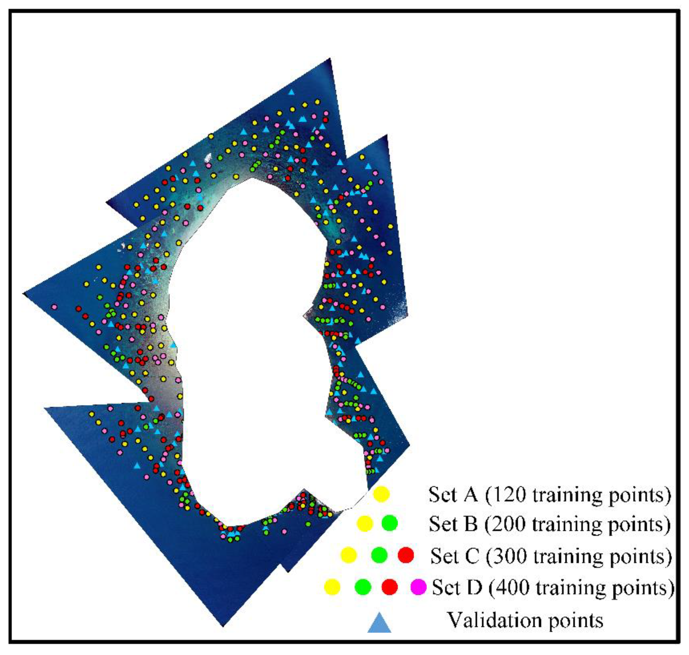
Figure 1. The relationships among the searching points, projection points, and projected centers in the ST method.
Remotesensing 14 00760 g001
Figure 2. The mosaic image of the experimental area composed by 5 projection images.
Remotesensing 14 00760 g002
Figure 3. Bathymetry derived by interpolating dense LiDAR points.
Remotesensing 14 00760 g003
Figure 4. Comparisons between LiDAR point depths and the 400 triangulation depths obtained by the ST method (a), and LiDAR depths and 400 calibrated depths derived by the combined approach (b).
Remotesensing 14 00760 g004
Figure 5. Distributions of reference points and validation points in 4 triangulation sets.
Remotesensing 14 00760 g005
Figure 6. Scatter plots of LiDAR points’ depths and the 120 estimation depths that are derived from 4 triangulation sets and 3 LiDAR sets. (a) Set A, (b) Set B, (c) Set C, (d) Set D, (e) Set E, (f) Set F and (g) Set G.
Remotesensing 14 00760 g006
Figure 7. Absolute residuals between the interpolation bathymetry of dense LiDAR points and the inferred bathymetries of 4 triangulation sets and 3 LiDAR sets. (a) Set A, (b) Set B, (c) Set C, (d) Set D, (e) Set E, (f) Set F and (g) Set G.
Remotesensing 14 00760 g007
Figure 8. MAE and RMSE of depth ranges corresponding to bathymetry derived by 3 LiDAR sets and 4 triangulation sets.
Remotesensing 14 00760 g008
Table 1. MAE and RMSE of the reference points of 4 triangulation sets when compared with their nearest LiDAR points.
4 Triangulation SetsSet ASet BSet CSet D
Reference points’ number120200300400
MAE (m)0.9971.2441.3711.595
RMSE (m)1.1651.4881.6311.843
Table 2. Inversion results of 4 triangulation sets and 3 LiDAR sets when compared to the estimation depths with LiDAR depths of 120 validation points.
Reference Points’ Number Set ASet BSet CSet DSet ESet FSet G
Triangulation Points as Reference PointsLiDAR Points as Reference Points
120200300400120200300
120 Validation points’ MAE (m)1.7131.3411.1181.0591.4711.2751.09
120 Validation points’ RMSE (m)2.3291.8241.4551.4062.0211.7651.417
Table 3. MAE and RMSE of the experimental area by comparing the interpolation bathymetry of dense LiDAR points and the inferred bathymetries of 4 triangulation sets and 3 LiDAR sets.
Set ASet BSet CSet DSet ESet FSet G
The experimental area’s MAE (m)2.312.2472.1291.9862.2932.1571.997
The experimental area’s RMSE (m)3.2873.2113.0642.8763.4323.1643.019
Table 4. The validation results of the MLR model combined with the ST method.
The Number of Reference Points120200300400
120 validation points’ MAE (m)2.0451.981.8941.948
120 validation points’ RMSE (m)2.6092.5732.5062.515
Publisher’s Note: MDPI stays neutral with regard to jurisdictional claims in published maps and institutional affiliations.

