Phenotypic Traits Extraction and Genetic Characteristics Assessment of Eucalyptus Trials Based on UAV-Borne LiDAR and RGB Images

Abstract

Phenotype describes the physical, physiological and biochemical characteristics of organisms that are determined or influenced by genes and environment. Accurate extraction of phenotypic data is a prerequisite for comprehensive forest phenotyping in order to improve the growth and development of forest plantations. Combined with the assessments of genetic characteristics, forest phenotyping will help to accelerate the breeding process, improve stress resistance and enhance the quality of the planted forest. In this study, we disposed our study in Eucalyptus trials within the Gaofeng forest farm (a typical Eucalyptus plantation site in southern China) for a high-throughput phenotypic traits extraction and genetic characteristics analysis based on high-density point clouds (acquired by a UAV-borne LiDAR sensor) and high-resolution RGB images (acquired by a UAV-borne camera), aiming at developing a high-resolution and high-throughput UAV-based phenotyping approach for tree breeding. First, we compared the effect of CHM-based Marker-Controlled Watershed Segmentation (MWS) and Point Cloud-based Cluster Segmentation (PCS) for extracting individual trees; Then, the phenotypic traits (i.e., tree height, diameter at breast height, crown width), the structural metrics (n = 19) and spectral indices (n = 9) of individual trees were extracted and assessed; Finally, a genetic characteristics analysis was carried out based on the above results, and we compared the differences between high-throughput phenotyping by UAV-based data and on manual measurements. Results showed that: in the relatively low stem density site of the trial (760 n/ha), the overall accuracy of MWS and PCS was similar, while in the higher stem density sites (982 n/ha, 1239 n/ha), the overall accuracy of MWS (F₍₂₎ = 0.93, F₍₃₎ = 0.86) was higher than PCS (F₍₂₎ = 0.84, F₍₃₎ = 0.74); With the increase of stem density, the difference between the overall accuracy of MWS and PCS gradually expanded. Both UAV–LiDAR extracted phenotypic traits and manual measurements were significantly different across the Eucalyptus clones (P < 0.05), as were most of the structural metrics (47/57) and spectral indices (26/27), revealing the genetic divergence between the clones. The rank of clones demonstrated that the pure clones (of E. urophylla), the hybrid clones (of E. urophylla as the female parent) and the hybrid clones (of E. wetarensis and E. grandis) have a higher fineness of growth. This study proved that UAV-based fine-resolution remote sensing could be an efficient, accurate and precise technology in phenotyping (used in genetic analysis) for tree breeding.

1. Introduction

Phenotype refers to the physical, physiological and biochemical characteristics such as morphology, structure, function of organisms under the combined action of genes and the environment [1,2]. Forest tree phenotype describes the comprehensive expression of height, yield, color, wood properties, stress resistance and other traits in the process of forest growth and development, it is the systematic measurement and characterization of different scales of forest (e.g., cells, organs, individuals, populations, forests, etc.) [3,4,5,6,7]. The analysis of phenotypes among forest trees can help accurately estimate the genetic characteristics, thereby improving our understanding of the adaptability of trees and their response to environmental changes, revealing the interaction between tree genes and the environment, as well as effectively correlating genotypes and phenotypes in forest trees for screening the target genes [8]. Although the genetic improvement of some conventional tree species has shown progress, there remains an imbalance between the breeding efficiency and the demands from commercial markets and ecological construction [9]. The development of precision silviculture and forest phenotyping requires the extraction and analysis of high-throughput, non-destructive and accurate data of forest phenotypic traits in order to quantify the genetic principles of specific phenotypes, accelerate forest tree breeding, improve the stress resistance of trees and systematically assess the internal relationship of “genotype–phenotype-environment” [10,11]. Eucalyptus are of great value for their contributions to industrial timber and pulpwood services in countries (e.g., Austria and China etc.) of the world due to its fast growth rate, barren-tolerance, wide adaptability and strong resistance. In Guangxi province, one of the key Eucalyptus plantation and industry provinces of China, the total planation area of Eucalyptus has exceeded 2 million ha, and the annual timber output has exceeded 21 million m³, accounting for approximately 1/4 of the national timber output. Therefore, Eucalyptus plays an important role in ensuring the national timber reserve and supply [12,13]. Although the improved breeding system has been developed in Guangxi province in recent years, the development of Eucalyptus planation remains restricted by challenges such as the degradation of Eucalyptus varieties, reduction of forest quality, and deceleration of yield growth etc. [14,15]. The recent advanced technology of high-throughput phenotypic trait extraction and statistical analysis of the genetic characteristics in forest trees is imperative for supporting genetic breeding of the precision silviculture.

At present, the accurate, precise and high-throughput acquisition of phenotypic traits as well as the development of the approaches for forest phenotyping is of great importance for genetic and tree breeding studies (and applications) [16,17]. The traditional forest phenotype acquisition commonly depends on manual measurements which is time-consuming and labor-intensive, and usually of a small scale with low efficiency, rendering it difficult to meet the needs of modern forest tree breeding. Advanced remote sensing technology, especially the rapidly developed UAV remote sensing system, provides an effective tool capable of obtaining real-time high-dimensional and -throughput phenotypic data with high-accuracy and high-spatial resolution. The phenotypic traits of forest trees can be estimated by combination with novel sensors, sophisticated image processing algorithms and advanced prediction models (e.g., artificial intelligence) [18,19,20]. UAV-borne LiDAR calculates the distance between the LiDAR sensor and the targets by recording the time interval to obtain high-density and high-precision three-dimensional point cloud data of the ground and forest canopy, which the can be used to visualize the 2D profile characteristics or 3D structural attributes of forest canopies [21]. The phenotypic traits such as tree height, crown width, DBH, volume, biomass, leaf area index can be directly extracted or indirectly obtained (e.g., predicted by inversion models), helping to provide insights into the structural changes and their response to changing environments in tree growth and development [22,23,24,25,26]. The UAV-borne RGB camera, as a convenient, economic and efficient tool for detecting tree crown and spectral reflectance in true color [27,28], can collect high-resolution images and detect the light reflectance variations to obtain the spectral characteristics of forest canopy [29,30]. Moreover, it has the potential to quantify the response of forest physiological and biochemical characteristics (e.g., leaf photosynthetic characteristics to environmental factors etc.) so as to effectively characterize the physiological and biochemical characteristics related to phenotypic traits of forest trees [31,32,33]. However, to the best of our knowledge, there are few studies that have assessed the capability of Eucalyptus phenotypic trait extraction for breeding, based on the advanced multi-source UAV data.

The extraction of forest phenotypic traits at an individual tree scale shows promise for genetic characteristic analysis of Eucalyptus trials and the selection of superior varieties. There are currently two main approaches for detecting individual trees by using LiDAR point clouds: approaches based on CHM (canopy height model) generated from LiDAR point cloud (e.g., Marker-controlled Watershed Segmentation (MWS) etc.) [34,35] and the approaches based on LiDAR point clouds directly (Point Cloud-based Cluster Segmentation (PCS), etc.) [36,37]. MWS sets a variable window that changes with the tree height and marks the local maximum of CHM as the crown treetop, then uses the watershed algorithm to determine the boundary of individual tree crowns. MWS usually bears strengths in recognizing crown boundaries capable of eliminating “false” crown vertices than ordinary watershed algorithms [38], while PCS judges and clusters a point cloud of individual trees by means of the top-down regional growth segmentation combined with threshold determination to judge the ownership of the target point.

In this study, we disposed a comprehensive UAV-based remote sensing campaign in the Eucalyptus trials of Gaofeng forest farm in Guangxi province of southern China. By using UAV-borne LiDAR data (of high-density point cloud) and RGB images (of high-resolution true-color orthophoto) collected by a multi-rotor UAV system, high-throughput phenotypic traits were extracted and analysis of genetic diversion was performed using the calculated results. The specific objectives of this study are: (1) to compare the accuracies of Marker-controlled Watershed Segmentation (MWS) and Point Cloud-based Cluster Segmentation (PCS) for detecting individual trees within the Eucalyptus trials and then extract phenotypic traits (i.e., tree height, diameter at breast height, crown width), the structural metrics (n = 19) and spectral indices (n = 9); (2) to analyze the genetic differences of the phenotypic traits, and the structural and spectral characteristics across the Eucalyptus clones, using the extracted results from the multi-source UAV remote sensing data. UAV–LiDAR extracted phenotypic traits and manually measured phenotypic traits were also compared to assess the effectiveness of the UAV technology for phenotypic analysis of forest trees.

2. Materials and Methods

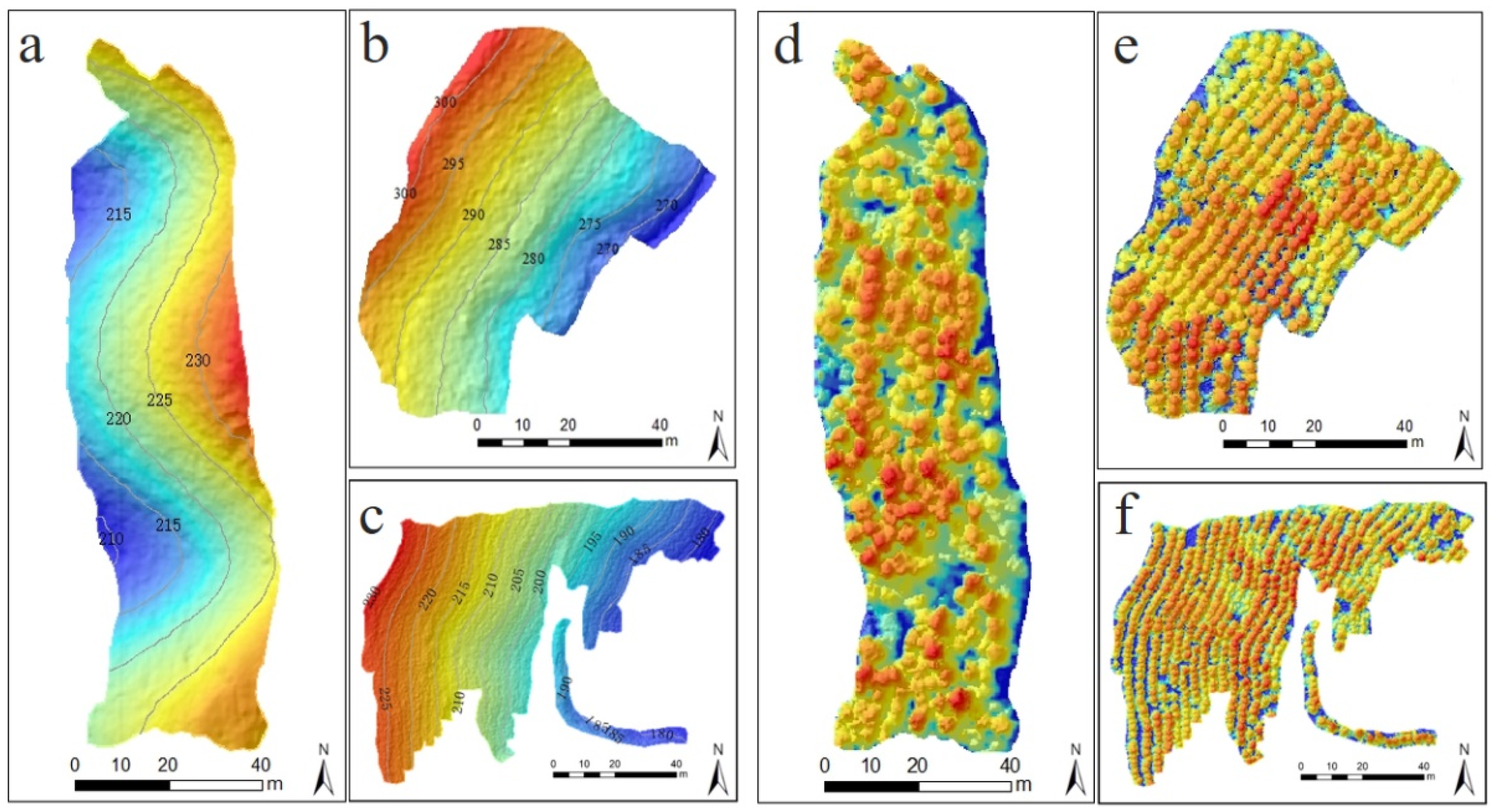
In this study, the Canopy Height Model (CHM) was generated based on the LiDAR point cloud obtained from the UAV platform, and the RGB orthophoto was generated based on the high-resolution true-color image. First, the segmentation accuracies of two individual tree segmentation algorithms (MWS and PCS) were evaluated based on the Canopy Height Model (CHM) and the normalized LiDAR point clouds, separately. The structural and spectral characteristics of individual trees in Eucalyptus trials were extracted according to the optimal individual tree segmentation results. Then, a statistical analysis was conducted to assess the genetic differences in phenotypic traits, structural and spectral characteristics. Finally, the genetic parameters were estimated and the superior clones and genetic gain were estimated. The workflow of this study is shown in Figure 1.

2.1. Study Area

The study sites are located within the clonal trials of Eucalyptus in the Gaofeng (State-owned) Forest Farm in Nanning city, Guangxi province (108°14′10″E, 22°56′10″N) of southern China. The local climate is the southern subtropical monsoon climate with sufficient sunshine and abundant rainfall. The annual average temperature is 21.6 °C, the minimum temperature is −2 °C, the maximum temperature is 40 °C, and the annual average precipitation ranges from 1200–1500mm, of which the precipitation from April to September accounts for 79.8% of the annual precipitation. The annual relative humidity is approximately 79% [39]. The topography of the study area is a hilly low mountain, with an altitude of approximately 180–250 m and an average slope of approximately 30°. The forest soil is lateritic red soil and the soil thickness is approximately 104–112 cm. The vegetations found below-canopy in the study sites-1 and -2 consists of relatively dense Dicranopteris dichotoma, Evodia lepta, Ficus esquiroliana, Clerodendrum cyrtophyllum, Microlepia hancei, etc. The understory vegetation in site-3 consists of relatively sparse Evodia lepta, Clerodendrum cyrtophyllum, Microlepia hancei, etc.

2.2. Study Materials

There are three sites of Eucalyptus trials in the study area. Trees in site-1 were planted in May 2015, with a total of 16 Eucalyptus clones including 12 Eucalyptus hybrid clones and 4 pure clones. Within site-1, there was set up in a randomized complete block design, with 4 rows × 5 plots, 3 replications, 48 plots in total. Trees in site-2 were planted in June 2016, with a total of 27 Eucalyptus clones including 21 Eucalyptus hybrid clones and 6 pure clones. Within site-2, there was set up in a randomized complete block design, with 4 rows × 5 plots. We measured trees in one of the replications. Eucalyptus in site-3 were planted in June 2018, with a total of 11 Eucalyptus pure clones. Within site-3, there was set up in a randomized complete block design, with 4 rows × 5 plots, 3 or 4 replications, 53 plots in total. See

Table A1. Information of Eucalyptus Clones.

Site	Number	Species	Site	Number	Species
1	EC176	E. wetarensis× (E. urophylla×E. wetarensis)	2	EC194	E. urophylla × E. pellita
	EC168	E. wetarensis× E. grandis		EC196	E. urophylla × E. pellita
	EC173	E. wetarensis× E. pellita		EC197	E. urophylla × E. pellita
	EC177	E. wetarensis× E. pellita		EC200	E. urophylla × E. pellita
	EC170	E. wetarensis× E. pellita		EC189	E. urophylla × E. camaldulensi
	JJ122	E. urophylla × E. wetarensis		JJ1402	E. urophylla
	EC174	E. urophylla		JJ1409	E. urophylla
	EC175	E. urophylla		JJ1410	E. urophylla
	JJ186	E. urophylla		JJ2280	E. urophylla
	JJ188	E. urophylla		EC182	E. grandis × E. urophylla
	EC151	E. wetarensis × E. grandis		GL9	E. grandis × E. urophylla
	EC171	E. wetarensis × E. grandis		EC184	E. grandis × E. grandis
	EC101	E. wetarensis × E. pellita		EC185	E. grandis × E. grandis
	EC169	E. wetarensis × E. pellita		EC195	E. pellita × E. urophylla
	SX93	E. camaldulensi		EC199	E. pellita × E. grandis
	SX96	E. camaldulensi		SX95	E. camaldulensi
2	EC180	E. wetarensis× E. urophylla	3	EC247	E. wetarensis × E. urophylla
	EC188	E. wetarensis× E. grandis		EC249	E. urophylla × E. wetarensis
	EC198	E.wetarensis× E. pellita		CM1605	E. urophylla × E. ABL
	3229	E. urophylla × E. grandis		CM1606	E. urophylla × E. ABL
	EC181	E. urophylla × E. grandis		CM1611	E. urophylla × E. ABL
	EC186	E. urophylla × E. pellita		CM1614	E. urophylla × E. ABL
	EC187	E. urophylla × E. pellita		CM1615	E. urophylla × E. ABL
	EC190	E. urophylla × E. pellita		EC254	E. wetarensis × (E. urophylla*E. pellita)
	EC191	E. urophylla × E. pellita		EC248	E. wetarensis × E. grandis
	EC192	E. urophylla × E. pellita		EC253	E. wetarensis × E. grandis
	EC193	E. urophylla × E. pellita		EC257	E. wetarensis

for Eucalyptus species information. The locations, Digital Elevation Models (DEMs) and Canopy Height Models (CHMs) are shown in Figure 2 and Figure 3.

2.3. Field Data and Manual Measurements

The ground survey was conducted in January 2020. The field measurements of a typical individual tree in each plot include diameter at breast height (DBH, measured with a diameter at a height of 1.3 m using a breast diameter ruler), tree height (H, using a Vertex ultrasonic altimeter), under-branch height, crown width (C, measured the width of north-south and east-west tree crowns with tape, and calculated the average value)) and positions (Trimble R6 GNSS (Trimble, Sunnyvale, CA, USA)). There were 40, 26, and 48 individual trees measured in site-1, 2, and 3, respectively.

In this study, the individual tree height and crown width derived from manually visual interpretation based on LiDAR high-density point cloud and high-resolution orthophoto combined with field data were regarded as manual measurements (LiDAR manually measured tree height (H1) and orthophoto interpreted crown width (C1) separately). First, the high-resolution orthophoto was registered to the CHM derived from LiDAR high-density point cloud, and the nearest neighbor pixel method was employed for resampling to obtain spatially matched CHM and RGB orthophoto. Then, we screened and located crowns of individual trees by means of zooming in to the orthophoto and CHM (normalized point clouds were also used as reference data), and drew circles with an average value of the lengths in 2 directions (i.e., the north–south and east–west directions) of each tree as the diameter to represent the crown. Finally, the diameters of each circle were calculated as the orthophoto interpreted crown width (C1), and the value of the highest point in CHM within each circular crown outline were extracted as the LiDAR manually measured tree height (H1).

To obtain the DBH of all individual trees, we established the DBH–H regression models by linear function, quadratic function, power function and exponential function using all field tree heights and DBH of individual trees from three sites. The optimal DBH–H model was selected to estimate individual tree DBH. The coefficient of determination (R²), root mean square error (RMSE) and relative root mean square error (rRMSE) were used to evaluate the DBH–H regression model as the following formula. The 10-fold cross-validation was performed to verify the accuracy of the DBH–H regression model. The original sample was randomly partitioned into 10 subsamples. Of the 10 subsamples, a single subsample was retained as the validation data for testing the model, and the remaining 9 subsamples were used as training data, then the average accuracy for 10 iterations was recorded as the final measurement [40].

$$R^2=1-\frac{{\displaystyle \sum _{i=1}^n}{\left(x_i-{\hat{x}}_i\right)}^2}{{\displaystyle \sum _{i=1}^n}{\left(x_i-{\stackrel{-}{x}}_i\right)}^2}$$

(1)

$$RMSE=\sqrt{\frac{1}{\mathrm{n}}\underset{i=1}{\sum ^n}{\left(x_i-{\hat{x}}_i\right)}^2}$$

(2)

$$rRMSE=\frac{RMSE}{{\stackrel{-}{x}}_i}\times 100\%$$

(3)

where $x_i$ is value of a phenotypic trait, ${\stackrel{-}{x}}_i$ is average value of a phenotypic trait; ${\widehat{x}}_i$ is the model estimated value of a phenotypic trait, n is the number of trees. The LiDAR manually estimated DBH (DBH1) was calculated based on the optimal DBH–H model and H1.

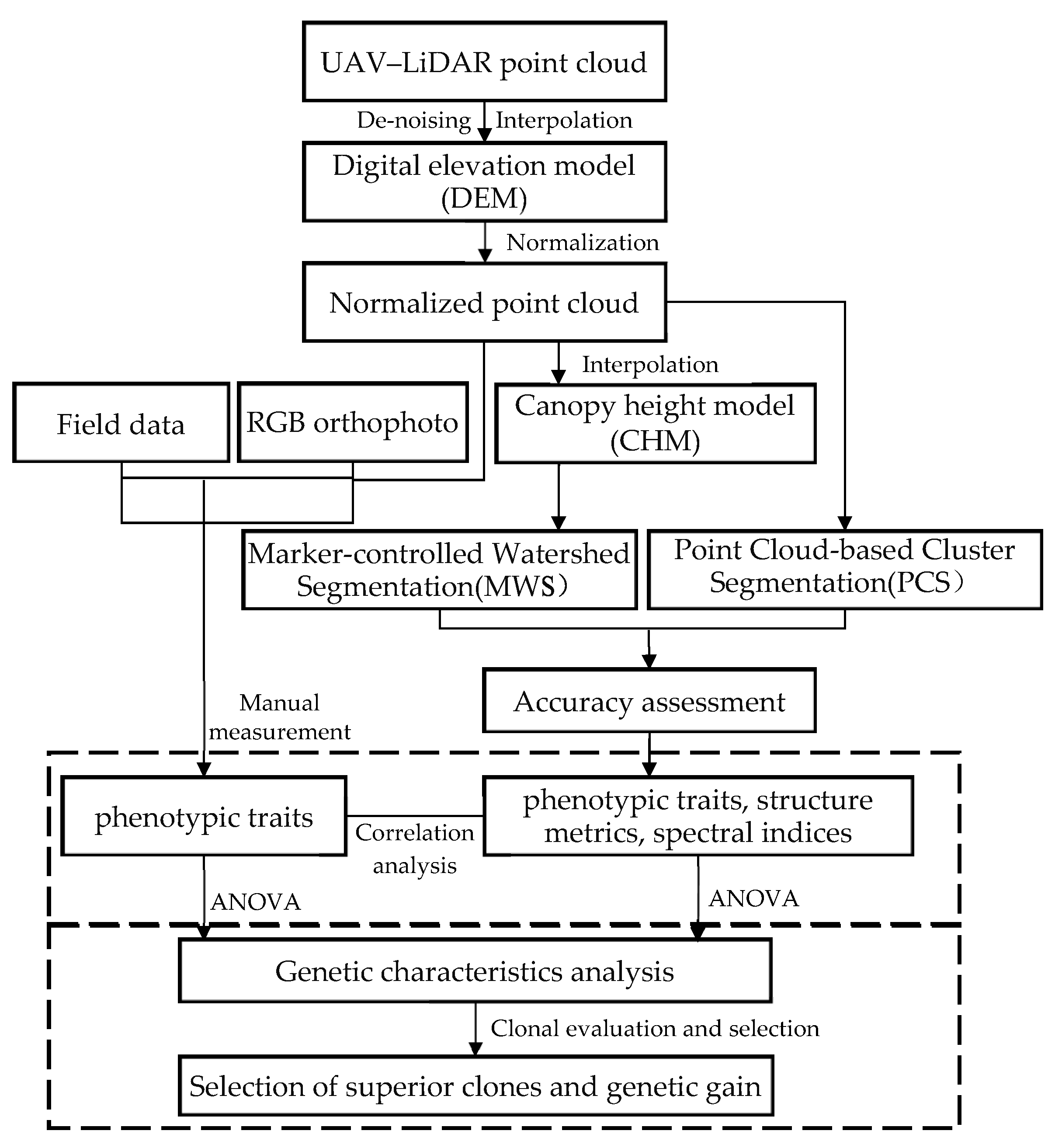
2.4. UAV-Borne LiDAR Data Acquisition and Preprocessing

The LiDAR data were obtained by RIEGL VUX-1LR carried by a multi-rotor UAV platform during 26–27 May 2020. The parameters of the UAV-borne LiDAR are as follows: flight altitude 250 m, flight speed 7 m/s, strip width 598.9 m, flight-direction overlap rate and side overlap rate 90%, scanning frequency 200 KHz, pulse emission frequency 820 KHz, divergence 0.5 mrad, laser footprint diameter 0.06 m, measurement accuracy 15 mm and an average point density of approximately 264.5 pts/m⁻².

LiDAR data preprocessing was as follows: First, we set a height threshold to remove noise in the original LiDAR data. Then, we classified and extracted ground points using an improved progressive encryption triangulated irregular network (TIN) densification filtering algorithm (IPTD) [41]. Next, we generated the Digital Elevation Model (DEM, 0.3 m) by inverse distance weighted interpolation (IDW). Finally, the Canopy Height Model (CHM, 0.3 m) from LiDAR point clouds was generated according to the DEM. The LiDAR metrics extracted from the normalized LiDAR point cloud include: distributional metrics (n = 13), Weibull-fitting metrics (n = 2), and canopy volume metrics (n = 4) (

Table 1. Description of the LiDAR metrics with equations and references separately.

Metrics	Description	Reference
Distributional metrics
h25, h50, h75, h95	The percentiles of the canopy height distributions by first echo (25th, 50th, 75th and 95th).	[42]
Hmean	The mean height of all points after normalized.	[42]
Hcv	The coefficient of variation of height of all points after normalized (the ratio of the standard deviation to the mean))	[42]
d1, d3, d5, d7, d9	The proportion of points above the quantiles (10th, 30th, 50th,70th, and 90th) to total number of points	[43]
CC2m	The first return points above 2 m accounts for the percentage of all return points	[42]
eLAI	Half of the total leaf area per unit ground area	[44]
Weibull-fitting metrics
α/β	The α and β parameter of the Weibull distribution fitted to foliage density profile.	[45]
Canopy volume metrics
Open gap zone (OP)/ Closed gap zone(CL)	The empty voxels located above and below the canopy respectively.	[46]
Euphotic zone (EU)/ Oligophotic zone (OL)	The voxels located within an uppermost percentile (65%) of all filled grid cells of that column, and voxels located below the point in the profile	[46]

)

2.5. UAV-Borne RGB Orthophoto Acquisition and Preprocessing

The RGB images were obtained by FC6310R carried by DJI-PHANTOM 4-RTK during 26–27 May 2020. The parameters were as follows: flight altitude 250 m, flight speed 10 m/s, flight-direction overlap rate and side overlap rate are about 80%, focal length 9 mm, exposure time 1/320 s, ISO 200, aperture value f/5.6, ground sampling distance (GSD) 6.85 cm.

The preprocessing of RGB images included the following: First, alignment of images with the help of five parameters (latitude, longitude, elevation, roll, pitch and heading) of each image recorded in real time by in-flight internal GPS data and inertial measurement units (IMUs). Then, the aligned images could be spliced and resampled together to generate a high-resolution true-color orthophoto (0.1 m) using Structure-from-Motion (SfM) image reconstruction. Finally, extraction of the pixel values of different bands at an individual tree scale based on the optimal individual tree segmentation. The vegetation indices calculated are shown in

Table 2. Description of visible vegetation indices (VI) with equations and references separately.

Vegetation Index	Equation	Reference
Brightness (BI)	G + R + B	[47]
NormG (NG)	G/(G + R + B)	[47]
RGRI	R/G	[48]
GRVI	(G − R)/(G + R)	[49]
VARI	(G − R) (G + R-B)	[50]
VDVI	(2G − (R + B))/(2G + (R + B))	[51]
EXG	(2G − R − B)/(R + G + B)	[52]
EXG-R	((3G − 2.4R − B)/(R + G + B)	[52]
CIVE	((0.411R − 0.811G + 0.385B)/(R + G + B)) + 18.787	[53]

Note: The vegetation indices were calculated using raw imagery bands; R, Red band; G, Green band; B, Blue band.

.

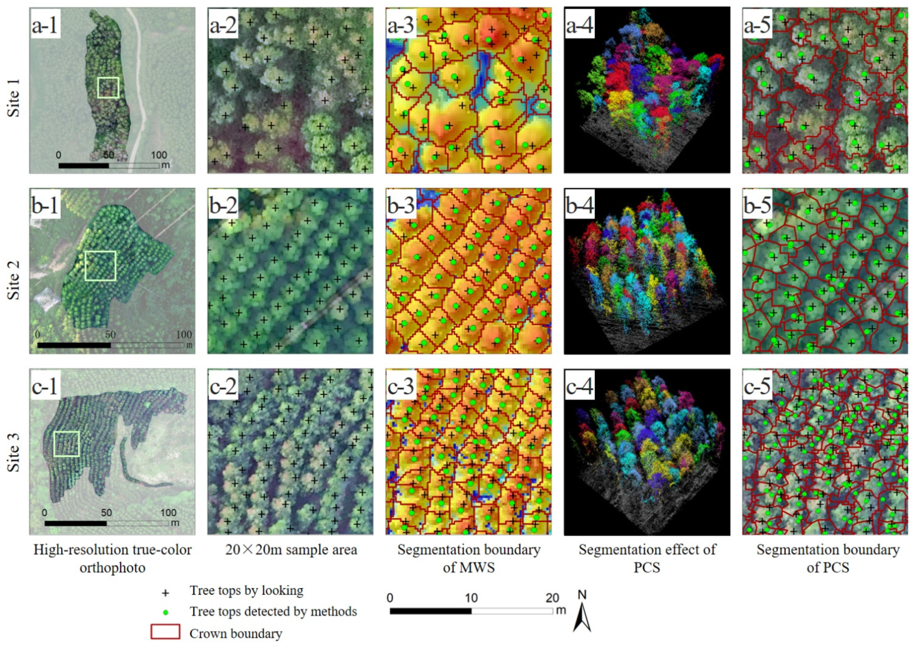
2.6. Individual Tree Segmentation Methods

Method 1: Marker-controlled Watershed Segmentation (MWS), First, the method generated the Canopy Maxima Model (CMM) by filtering CHM with variable window sizes determined by the lower-limit of the prediction intervals of the regression curve between crown size and tree height. Then, the treetops were detected and marked by searching local maxima in a smoothed CMM with variable window sizes. Next, the initial delineation of tree crowns was segmented using marker-controlled watershed segmentation, it is assumed that water is injected from each marked treetop, and the water is gradually immersed to form multiple “ponding basins”, the region of each marked treetop is surrounded by the corresponding “dam” as the initial delineation of tree crowns after segmentation. Lastly, the final tree crowns are obtained by distance transformation [54,55].

Method 2: Point Cloud-based Cluster Segmentation (PCS). The principle of PCS is top-down regional growth combined with threshold determination based on normalized point clouds directly. This approach sets the horizontal distance as the threshold between tree vertices according to the phenomenon of certain distance between trees. First, to assume that the highest point in the normalized LiDAR point cloud is the tree vertex, and judge distance iteratively from tree vertex to bottom: If the horizontal distance between the target point and the vertex of individual tree is greater than the threshold, the target point belongs to another individual tree point cloud cluster; If not, the ownership of the target point is determined through additional filter rules. Finally, the steps are repeated until the bottom points are segmented [34,37]. The accuracy evaluation indexes of individual tree segmentation were as follows [56,57].

$$r=\frac{N_t}{N_t+N_o}$$

(4)

$$p=\frac{N_t}{N_t+N_c}$$

(5)

$$F=\frac{2\left(r \times p\right)}{r+p}$$

(6)

where r represents the tree detection rate, p represents the tree detection accuracy, and F represents the overall accuracy taking both omission and commission into consideration. N_t is the number of trees detected by the algorithm and corresponds to the measured trees in the field. N_O is the number of trees that cannot be detected by the algorithm but exist in the field. N_C is the number of trees detected by the algorithm but do not exist in the field.

2.7. Statistical Analysis Methods

In this study, the phenotypic traits (tree height, crown width) of individual trees were extracted using the optimal individual tree segmentation result as the LiDAR extracted tree height (H2) and LiDAR extracted crown width (C2). The LiDAR estimated DBH (DBH2) was derived from the optimal DBH–H model and H2. Based on the above results. Scatter plots were used to compare the UAV–LiDAR extracted phenotypic traits, measured data and manual measurements. The correlations between phenotypic traits and LiDAR metrics and vegetation index were compared by Pearson correlation coefficient.

Statistical analysis was then performed on the phenotypic traits and the structural, spectral characteristics to analyze the differences across the Eucalyptus clones and the relationship between Eucalyptus phenotypic traits and structural, spectral characteristics. Variations among clones within these sites were analyzed by ANOVA using following linear mixed model: $X_{ijk}{=\mu +C}_i{+B}_j{+CB}_{ij}{+\epsilon }_{ijj}$, where $X_{ijk}$ represents the phenotypic value of an individual tree k of clone i in replication j, μ represents the overall mean, C_i represents genetic effect (random) of clone i, B_j represents effect (fixed) of replication j, and CB_ij represents the interaction effect (random) of clone i and replication j, ε_ijk represents random error. The restricted or residual maximum likelihood algorithm (REML) was used to perform variance component estimation for the statistical analysis. The genetic parameters of Eucalyptus phenotypic traits and preferred three indexes include phenotypic coefficients of variation (PCV), genotypic coefficients of variance (GCV), repeatability of clones (R_c), and repeatability of individual trees (R_i) [58,59,60] were estimated by the following formula:

$$PCV=\frac{\sqrt{{\sigma }_c^2{+\sigma }_{\mathrm{cr}}^2{+\sigma }_e^2}}{\stackrel{-}{X}}\times 100\%$$

(7)

$$GCV=\frac{\sqrt{{\sigma }_c^2}}{\stackrel{-}{X}}\times 100\%$$

(8)

$$R_c=\frac{{\sigma }_c^2}{{\sigma }_c^2+{\sigma }_w^2/r}$$

(9)

$$R_i=\frac{{\sigma }_c^2}{{\sigma }_c^2+{\sigma }_w^2}$$

(10)

where $\stackrel{-}{X}$ is the mean value of the trait, ${\sigma }_c^2$ is the clonal variance component, ${\sigma }_{cr}^2$ is the interaction of the replication and the clone variance, ${\sigma }_e^2$ is the residual variance component, ${\sigma }_w^2$ is the environment variance component, $r$ is the number of replications. Repeatability, the ideal heritability in a broad sense for a trait ranged from 0 to 1, can indicate the stability of gene expression of a trait in a fluctuating environment, the higher the repeatability, the greater the influence of gene on phenotypic traits, and the more reliable the clonal selection [61,62,63,64].

An improved method of multi-trait comprehensive evaluation was used to assess the clones according to the phenotypic traits extracted from the remote sensing data and the photogrammetric data use of Eucalyptus as pulpwood. Tree height and DBH were the most important traits in the process of superior material evaluation. The formula used was as follows [65]:

$$Q_i=\sum K_j\left(1-\frac{X_{ij}}{X_0}\right)$$

(11)

where $Q_i$ is the comprehensive evaluation value of each clone ranged between 0 and 1, the smaller the value of $Q_i$, the higher the excellence of the clone, $K_j$ is the weight set by the importance of phenotypic traits and the use of Eucalyptus as pulp wood in this study, $K_j$ = (H, DBH, C) = (0.6, 0.3, 0.1), $X_{ij}$ is the average value of one trait, $X_0$ is the maximum value of the trait, n is the number of traits. The $Q_{i1}$ thereby was calculated based on manual measurements (i.e., H1, DBH1 and C1) and the $Q_{i2}$ was calculated based on LiDAR extracted phenotypic traits (i.e., H2, DBH2 and C2).

Genetic gain, closely related to the level of repeatability and the degree of trait variation, represents the improvement effect of selection. The genetic gain was estimated using the following formula [66,67]:

$$\Delta G=\frac{\left(\stackrel{-}{x}-\stackrel{-}{X}\right){\times R}_c}{\stackrel{-}{X}} \times 100$$

(12)

where $R_c$ is the repeatability of clone; $\stackrel{-}{x}$ is mean of selected clones; and $\stackrel{-}{X}$ is the mean value of all parent. In this study, the mean value of all tested clones was used to represent the mean value of all parents at each site [63].

3. Results

3.1. Individual Tree Segmentation

The effects of individual tree segmentation are shown in Figure 4. The manually interpreted crown vertices and the crown boundaries were displayed, as well as crown vertices obtained by the two segmentation methods. In the three sites, the average canopy widths were 4.16 m, 3.38 m, and 3.06 m, respectively, while the stem density were 760 n/ha, 982 n/ha, 1239 n/ha, respectively. The canopy boundaries depicted by MWS with better visual effect are closer to the actual canopy boundaries than PCS. In the low density site-1, the overall accuracy(F) of MWS and PCS was similar, whereas the tree detection rate of MWS (r₍₁₎ = 0.74) was lower than PCS (r₍₁₎ = 0.87), the tree detection accuracy of MWS (p₍₁₎ = 0.87) was higher than PCS (p₍₁₎ = 0.73). In the higher-density sites-2 and -3, both MWS and PCS had the higher over-segmentation phenomenon (N_C) than the missing segmentation phenomenon (N_O), while the tree detection rate and tree detection accuracy of MWS (r₍₂₎ = 0.94, r₍₃₎ = 0.92, p₍₂₎ = 0.92, p₍₃₎ = 0.81) were higher than PCS (r₍₂₎ = 0.93, r₍₃₎ = 0.84, p₍₂₎ = 0.76, p₍₃₎ = 0.67). With the increase of forest stem density in three sites, the difference between the overall accuracy of MWS and PCS gradually expanded (

Table 3. The accuracy assessments for the individual tree segmentation algorithms of MWS and PCS.

Site	Stem Density (n/ha)	Crown Width (m)	Method	Nt	NO	NC	r	p	F
1	760	max = 6.67 mean = 4.18 min = 2.06	MWS	278	98	42	0.74	0.87	0.80
			PCS	327	49	118	0.87	0.73	0.80
2	982	max = 4.54 mean = 3.38 min = 2.14	MWS	343	20	31	0.94	0.92	0.93
			PCS	338	25	105	0.93	0.76	0.84
3	1239	max = 4.06 mean = 3.05 min = 2.18	MWS	632	57	145	0.92	0.81	0.86
			PCS	581	108	291	0.84	0.67	0.74

Note: MWS: Marker-controlled Watershed Segmentation; PCS: Point Cloud-based Cluster Segmentation; N_t, N_O, N_C, r, p, F are described in Equations (4)–(6).

). The segmentation results of MWS were selected for subsequent analysis based on the above results.

3.2. Statistical Analysis

3.2.1. Diameter at Breast Height (DBH)—Tree Height (H) Regression Model

The correlation coefficient value (r) calculated between the field measured tree height and the field measured DBH was 0.89. The results of accuracy assessments and cross-validation show that the DBH–H regression model established by exponential function fitted best (R² = 0.78) (

Table 4. The results of accuracy assessments and cross-validation of DBH-tree height regression model.

Functions	Models	R2	RMSE/cm	rRMSE/%	Cross-Validation
					R2	RMSE/cm	rRMSE/%
Linear function	D = 0.7175 H + 1.5791	0.80	1.50	13.74	0.77	1.54	14.12
Quadratic function	D = −0.0187 H2 + 1.2227 H − 1.5491	0.78	1.54	14.10	0.76	1.55	14.22
Power function	D = 1.2152 H0.8547	0.80	1.50	13.74	0.76	1.53	14.03
Exponential function	D = 4.3920 e0.0668H	0.81	1.48	13.56	0.78	1.51	13.85

Note: D, predicted DBH (cm); H. Tree height (m).

). We chose the DBH–H regression model established by exponential function to predicted individual tree DBH. The DBH1 was derived from the DBH–H regression model and H1, and the DBH2 was derived from DBH–H regression model and H2.

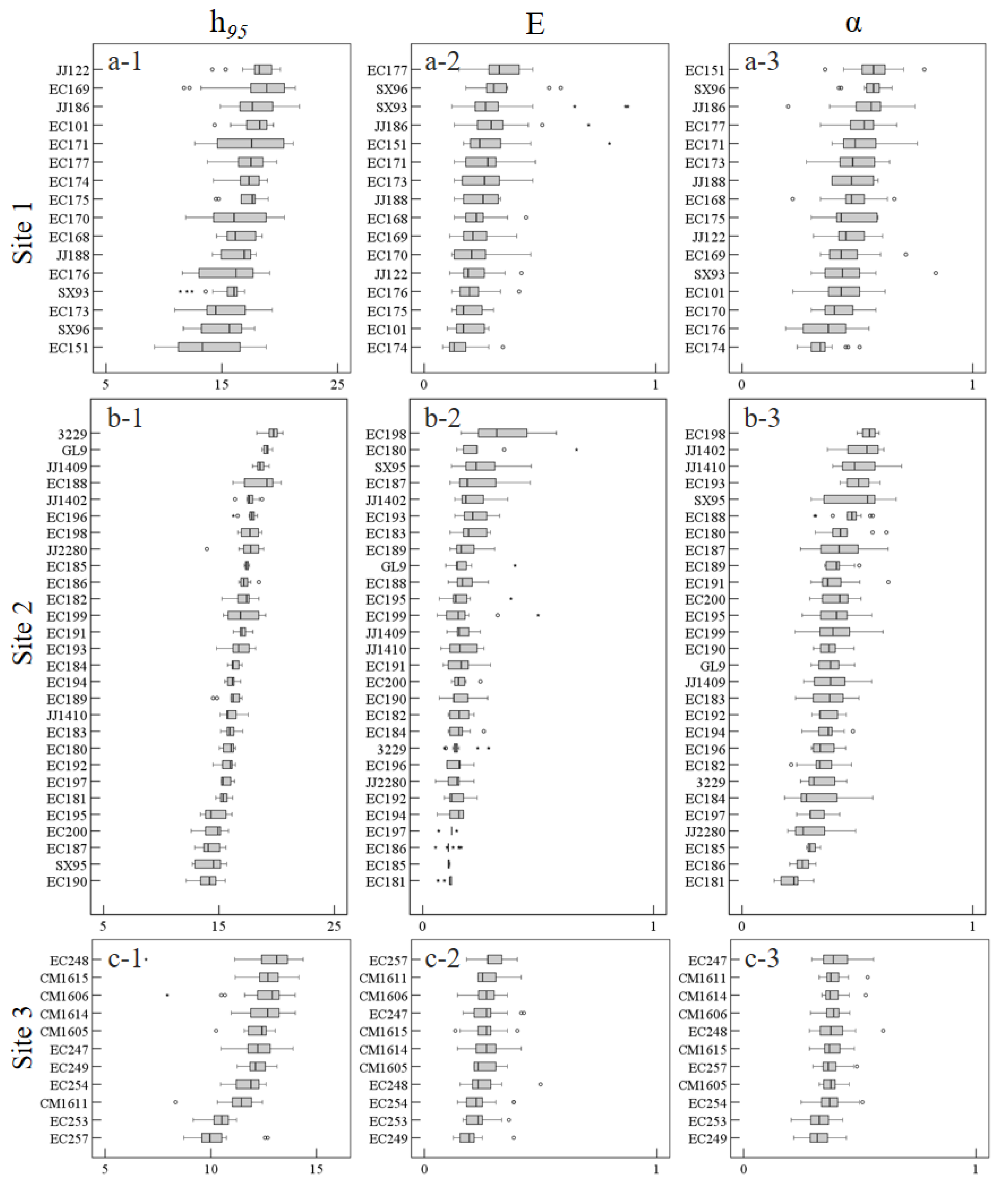
3.2.2. Phenotypic Traits and Analysis

Scatter plots of LiDAR extracted phenotypic traits and field measurements, manual measurements in the three sites showed that the LiDAR extracted tree height (H2) was higher than field-measured tree height while the R² is 0.55, 0.68, 0.53, respectively. In the comparison between LiDAR extracted phenotype traits and manual measurements, the H2 were highly correlated with the H1 (r > 0.94, R² > 0.91), as well as the DBH2 and DBH1 (r > 0.94, R² > 0.91), but correlations between the C2 and C1 were rather low for r ranging from 0.42 to 0.80 (Figure 5). The results of correlations between different phenotypic traits showed that there was a strong correlation between tree height and DBH, as the DBH was obtained from the DBH–H regression model, while the correlations between crown width and DBH, tree height were low (

Table A3. Pearson’s correlations between phenotypic traits and LiDAR metrics and vegetation index in three sites.

Correlation		Site-1						Site-2						Site-3
		H1	H2	D1	D2	C1	C2	H1	H2	D1	D2	C1	C2	H1	H2	D1	D2	C1	C2
Traits	H1		0.95 **	0.99 **	0.95 **	0.52 **	0.48 **		0.99 **	1.00 **	0.99 **	0.22 **	0.26 **		0.96 **	0.98 **	0.96 **	0.25 **	0.35 **
	H2	0.95 **		0.95 **	0.99 **	0.57 **	0.53 **	0.99 **		0.99 **	1.00 **	0.22 **	0.27 **	0.96 **		0.96 **	1.00 **	0.24 **	0.34 **
	D1	0.99 **	0.95 **		0.95 **	0.52 **	0.48 **	1.00 **	0.99 **		0.99 **	0.22 **	0.26 **	1.00 **	0.96 **		0.96 **	0.25 **	0.35 **
	D2	0.95 **	0.99 **	0.95 **		0.56 **	0.53 **	0.99 **	1.00 **	0.99 **		0.68 **	0.92 **	0.96 **	0.98 **	0.96 **		0.24 **	0.34 **
	C1	0.52 **	0.57 **	0.52 **	0.56 **		0.80 **	0.22 **	0.22 **	0.22 **	0.68 **		0.74 **	0.25 **	0.24 **	0.25 **	0.24 **		0.63 **
	C2	0.48 **	0.53 **	0.48 **	0.53 **	0.80 **		0.26 **	0.27 **	0.26 **	0.92 **	0.74 **		0.35 **	0.34 **	0.35	0.34	0.63 **
LiDAR metrics	Hmean	0.76 **	0.77 **	0.52 **	0.37 **	0.16 **	0.17 **	0.68 **	0.69 **	0.39 **	0.18 **	0.03	−0.12 *	0.80 **	0.84 **	0.51 **	0.37 **	0.10	0.02
	Hcv	0.23 **	0.21 **	0.24 **	0.30 **	0.28 **	0.19 **	0.03	0.04	0.02	0.21 **	0.02	0.25 **	0.14 *	0.12 *	0.00	0.23 **	−0.09	0.22 **
	h25	0.43 **	0.46 **	0.25 **	0.11	−0.03	0.03	0.35 **	0.04 **	0.18 **	−0.02	−0.02	−0.21 **	0.63 **	0.66 **	0.43 **	0.23 **	0.13 *	−0.06
	h5	0.67 **	0.69 **	0.45 **	0.28 **	0.08	0.14 *	0.70 **	0.71 **	0.34 **	0.16 **	−0.05	−0.16 **	0.76 **	0.79 **	0.47 **	0.32 **	0.09	−0.03
	h75	0.90 **	0.90 **	0.65 **	0.51 **	0.28 **	0.27 **	0.94 **	0.95 **	0.56 **	0.44 **	0.08	0.06	0.90 **	0.93 **	0.57 **	0.47 **	0.07	0.10
	h95	0.99 **	0.95 **	0.69 **	0.68 **	0.46 **	0.29 **	0.99 **	0.99 **	0.66 **	0.58 **	0.18 **	0.22 **	0.94 **	0.99 **	0.57 **	0.58 **	0.08	0.20 **
	d3	0.20 **	0.17 **	0.06	0.12	0.09	−0.05	0.08	0.08	0.06	−0.15 **	0.02	−0.23 **	0.13 *	0.14 *	0.22 **	−0.08	0.20 **	−0.17 **
	d5	0.08	0.09	−0.04	−0.08	−0.12	−0.13 *	0.10	0.10	0.04	−0.20 **	−0.03	−0.30 **	0.18 **	0.18 **	0.20 **	−0.14 *	0.13 *	−0.27 **
	d7	0.03	0.09	−0.03	−0.22 **	−0.28 **	−0.11	0.10	0.10	-0.03	-0.28 **	−0.11 *	−0.40 **	0.16 **	0.16 **	0.17 **	−0.20 **	0.10	−0.34 **
	d9	0.06	0.137 *	0.04	−0.27 **	−0.36 **	−0.05	0.01	0.02	−0.24 **	−0.46 **	−0.34 **	−0.57 **	0.07	0.08	0.03	−0.25 **	−0.02	−0.36 **
	OP	0.30 **	0.23 **	0.35 **	0.49 **	0.51 **	0.32 **	−0.01	−0.01	0.31 **	0.48 **	0.42 **	0.60 **	0.08	0.08	0.14 *	0.32 **	0.11	0.36 **
	EU	−0.19 **	−0.16 **	−0.15 *	−0.12 *	−0.11	−0.11	−0.02	−0.03	0.07	0.20 **	0.12 *	0.27 **	−0.02 **	−0.14 *	−0.15 **	0.09	−0.08	0.19 **
	OL	−0.16 **	−0.12 *	−0.21 **	−0.33 **	−0.34 **	−0.21 **	0.01	0.02	−0.34 **	−0.54 **	−0.48 **	−0.68 **	0.06	0.05	0.00	−0.30 **	−0.03	−0.40 **
	CL	0.07	0.07	0.05	0.02	0.00	0.02	0.01	0.00	0.22 **	0.28 **	0.29 **	0.34 **	0.01	0.00	0.06	0.14 *	0.05	0.17 **
	α	−0.38 **	−0.49 **	−0.21	−0.38 **	0.02	−0.28	−0.06	−0.07	0.08	0.33 **	0.15 **	0.44 **	−0.03	−0.02	−0.10	0.28 **	−0.10	0.37 **
	β	−0.50 **	−0.55 **	−0.44 **	−0.44 **	−0.22	−0.31 *	−0.12 *	0.00	0.16 **	0.35 **	0.31 **	0.51 **	−0.15 **	−0.15 **	−0.07	0.21 **	0.01	0.35 **
	LAI	0.24	0.37 **	0.10	0.40 **	−0.06	0.36 *	0.24	−0.14 *	0.21 *	0.21	−0.05	0.32	0.26 *	0.29 *	0.14	0.37 **	−0.11	0.35 **
	CC2	0.23	0.38 **	0.13	0.46 **	−0.02	0.43 **	0.29 *	0.32 *	0.13	0.10	−0.11	0.43 **	0.24	0.40 **	0.31 *	0.49 **	−0.10	0.30
VI	BI	0.21 **	0.25 **	0.21 **	0.06	0.00	0.13 *	−0.08	−0.07	0.05	0.08	0.12 *	0.14 *	−0.04	−0.03	−0.05	0.13 *	−0.03	0.19 **
	NG	0.10	0.10	0.12	0.126 *	0.121 *	0.08	0.08	0.08	0.01	0.07	−0.04	0.06	0.07	0.07	−0.16 **	0.26 **	−0.25 **	0.29 **
	RGRI	0.09	0.11	0.05	−0.03	−0.08	0.01	−0.19 **	−.19 **	0.03	−0.04	0.17 **	0.04	−0.05	−0.04	0.20 **	−0.30 **	0.29 **	−0.35 **
	GRVI	−0.10	−0.12	−0.06	0.03	0.07	−0.01	−0.08	−0.08	0.00	−0.07	0.04	−0.05	−0.08	−0.07	0.15 **	−0.26 **	0.25 **	−0.29 **
	VARI	−0.16 **	−0.18 **	−0.11	0.00	0.06	−0.04	0.07	0.06	0.00	0.00	−0.05	−0.05	−0.10	−0.09	0.12 *	−0.24 **	0.22 **	−0.25 **
	VDVI	0.10	0.10	0.12	0.127 *	0.121 *	0.08	−0.18 **	−0.18 **	0.05	−0.03	0.19 **	0.05	−0.05	−0.04	0.19 **	−0.30 **	0.29 **	−0.35 **
	EXG	0.10	0.10	0.12	0.126 *	0.120 *	0.08	−0.18 **	−0.18 **	0.05	−0.03	0.19 **	0.06	−0.05	−0.04	0.20 **	−0.30 **	0.29 **	−0.35 **
	EXGR	0.01	0.00	0.04	0.08	0.10	0.04	−0.15 **	−0.15 **	0.03	−0.05	0.14 *	0.01	−0.06	−0.05	0.18 **	−0.29 **	0.28 **	−0.33 **
	CIVE	−0.09	−0.09	−0.11	−0.12 *	−0.12	−0.07	0.18 **	0.18 **	−0.06	0.03	−0.19 **	−0.04	0.05	0.04	−0.20 **	0.30 **	−0.29 **	0.35 **

Note: *: significant correlations (P < 0.05); **: extremely significant correlations (P < 0.01).

).

The site-1 would be selected as the low-density site and the site-3 would be chosen as the high-density site for the following statistical analysis (assessments of genetic parameters were not conducted in site-2 as there was no data collected from other replications). The results of ANOVAs showed that there were significant (P < 0.05) differences in phenotypic traits among clones, which indicated there was genetic divergence in phenotypic traits and it was feasible to evaluate and select superior clones (

Table 5. F-values and significance levels of ANOVAs from different sources for phenotypic traits of three sites.

Types of Variation	H1 (m)	H2 (m)	DBH1 (cm)	DBH2 (cm)	C1 (m)	C2 (m)
Low-densitysite
Mean ± std	17.49 ± 1.9	17.08 ± 1.96	14.32 ± 1.73	13.93 ± 1.73	4.22 ± 0.52	4.18 ± 0.69
Replication	0.32	0.93	0.43	1.06	2.88	0.87
Clone	2.25 *	2.63 *	2.16 *	2.41 *	2.11 *	2.22 *
Clone × replication	3.71	10.12	3.21	8.82	61.76	0.38
High-density site
Mean ± std	12.29 ± 1.00	12.27 ± 1.05	10.02 ± 0.66	10.01 ± 0.69	3.05 ± 0.39	4.09 ± 0.46
Replication	1.76	1.07	1.84	1.23	1.32	4.30 **
Clone	8.59 **	9.68 **	8.42 **	9.22 **	2.84 *	3.59 **
Clone × replication	3.02	2.04	3.55	1.98	3.42	2.90

Note: *: significant difference (P < 0.05); **: extremely significant difference (P < 0.01). H1, LiDAR manually measured tree height; H2, LiDAR extracted tree height; DBH1, LiDAR manually estimated DBH; DBH2, LiDAR estimated DBH; C1, orthophoto interpreted crown width; C2, LiDAR extracted crown width.

).

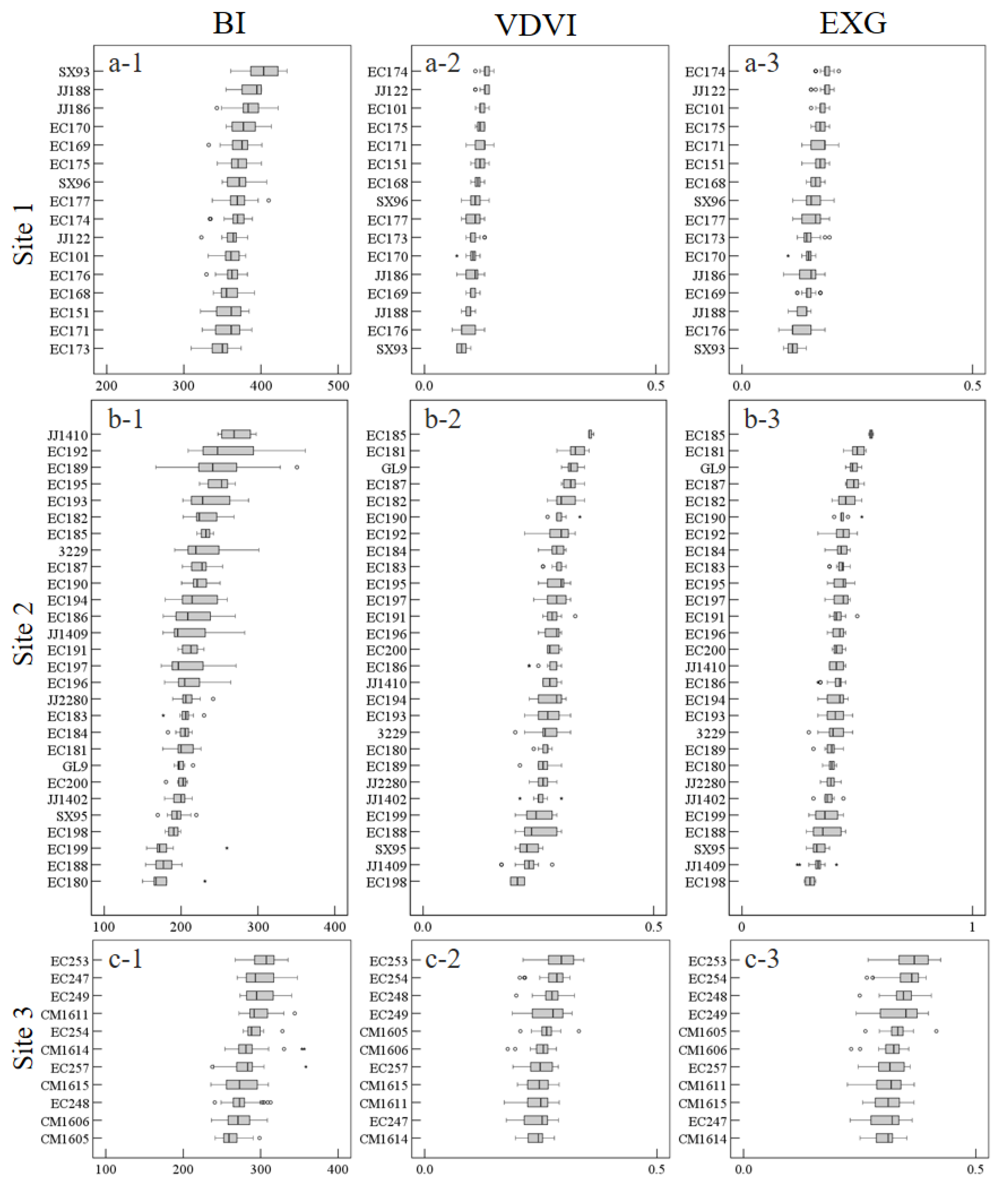
3.2.3. LiDAR Metrics and Vegetation Indices Extraction and Analysis

Most of the LiDAR Metrics (47/57) and visible vegetation indices (26/27) differed significantly among clones in the three sites (P < 0.01) (

Table A2. F-value and significance level of ANOVAs for LiDAR metrics and vegetation index (VI) in three sites.

Mstrics		Site-1				Site-2		Site-3
		Mean ± std	Clone	rep	Clone × rep	Mean ± std	Clone	Mean ± std	Clone	rep	Clone × rep
LiDAR metrics	Hmean	12.02 ± 1.99	3.38 **	1.60	2.16	12.95 ± 1.88	15.87 **	8.98 ± 0.96	3.22 **	0.30	8.33 **
	Hcv	0.32 ± 0.06	2.51 *	1.34	3.81	0.31 ± 0.11	6.15 **	12.78 ± 1.21	2.75 *	3.01 *	2.40 **
	h25	10.14 ± 1.52	3.52 **	3.59 *	2.32	11.01 ± 3.39	6.71 **	0.27 ± 0.04	2.06 *	0.52	7.68 *
	h5	13.11 ± 1.73	2.69 **	1.69	4.43	14.32 ± 2.04	14.03 **	7.49 ± 1.04	3.02 **	0.53	8.34 **
	h75	15.16 ± 1.85	2.587 *	1.40	2.90	15.78 ± 1.68	29.56 **	9.41 ± 1.11	4.77 **	0.15	7.49 **
	h95	16.64 ± 1.82	3.19 **	0.54	3.27	16.69 ± 1.67	37.29 **	10.89 ± 1.08	7.00 **	0.61	5.69 **
	d3	0.62 ± 0.10	8.06 **	2.29	61.22	0.63 ± 0.10	8.94 **	0.74 ± 0.07	1.51	2.66 *	3.40 **
	d5	0.52 ± 0.10	6.17 **	4.69 *	266.02 *	0.58 ± 0.12	9.36 **	0.62 ± 0.09	0.90	2.47 *	5.43 **
	d7	0.37 ± 0.09	4.28 **	2.64	98.50	0.51 ± 0.13	11.25 **	0.4 ± 0.09	1.31	3.32 *	5.68 **
	d9	0.13 ± 0.04	2.28 *	2.83	0.95	0.22 ± 0.09	6.33 **	0.09 ± 0.04	1.48	2.57 *	2.61 **
	OP	0.21 ± 0.11	0.02 *	3.05	15.18	0.07 ± 0.15	3.22 **	0.01 ± 0.04	2.76 **	0.64	3.76 **
	EU	0.28 ± 0.10	0.00 **	2.47	35.07	0.18 ± 0.08	4.34 **	0.25 ± 0.06	1.97 **	2.09	3.35 **
	OL	0.46 ± 0.13	0.22	4.61 *	1325.86 *	0.70 ± 0.20	3.09 **	0.72 ± 0.09	1.27 *	2.18	5.38 **
	CL	0.06 ± 0.06	0.01 *	0.15	2.62	0.05 ± 0.08	3.09 **	0.01 ± 0.05	2.55 *	0.93	3.00 **
	α	0.56 ± 0.11	5.67 **	7.02 **	0.62	0.38 ± 0.11	8.98 **	0.37 ± 0.06	0.71 *	2.28	7.07 *
	β	1.79 ± 1.05	2.44 *	3.27	3.65	1.08 ± 0.19	6.29 **	1.50 ± 0.17	1.59 *	3.44	2.73 *
	LAI	2.28 ± 0.63	4.04 **	3.05	2.21	2.70 ± 0.15	-	2.45 ± 0.19	0.84	0.32	1.71
	CC	0.64 ± 0.18	5.58 **	0.89	10.96	0.687 ± 0.01	-	0.70 ± 0.01	0.70	0.49	1.02
VI	BI	373.84 ± 16.88	4.50 **	3.64 *	0.41	345.24 ± 20.22	9.75 **	373.84 ± 16.88	3.93 **	5.74 **	9.20 **
	NG	0.39 ± 0.01	6.23 **	0.73	-	0.71 ± 0.01	7.97 **	0.39 ± 0.01	3.30 **	2.17	13.81 **
	RGRI	0.78 ± 0. 03	4.39 **	0.04	0.94	0.85 ± 0. 03	16.86 **	0.78 ± 0. 03	4.29 **	5.28 **	11.04 **
	GRVI	0.13 ± 0.02	4.34 **	0.03	0.76	0.14 ± 0.02	8.34 **	0.13 ± 0.02	3.60 **	2.53	13.04 **
	VARI	0.15 ± 0.03	1.61	0.76	3.80	0.15 ± 0.05	9.06 **	0.15 ± 0.03	3.45 **	1.73	11.82 **
	VDVI	0.11 ± 0.02	6.25 **	0.67	193.83	0.10 ± 0.01	16.01 **	0.11 ± 0.02	4.17 **	4.81 **	12.13 **
	EXG	0.16 ± 0.02	6.09 **	0.71	405.46	0.16 ± 0.02	17.23 **	0.16 ± 0.02	4.29 **	5.35 **	11.90 **
	EXG-R	0.12 ± 0.04	5.54 **	0.15	4.25	0.12 ± 0.03	11.88 **	0.12 ± 0.04	3.96 **	3.97 **	13.59 **
	CIVE	18.71 ± 0.01	6.28 **	0.61	-	16.48 ± 0.08	15.59 **	18.71 ± 0.01	4.06 **	4.71 **	11.37 **

Note: *: significant difference (P < 0.05); **: extremely significant difference (P < 0.01).

). We then screened six indicators with significant differences (h₉₅, E, α, BI, VDVI, EXG) to make box plots for showing the differences among different clones (Figure 6 and Figure 7). The correlation analysis results showed that the phenotypic traits had significant but weak correlation with most LiDAR metrics, while the phenotypic traits value had no significant correlation with most vegetation indices (Table A3).

3.3. Genetic Parameters and Clone Evaluation

In the low-density site, the PCV and GCV ranged from 0.062 to 0.169 and the R_c of the different phenotypic traits was moderate or high (varied from 0.537 to 0.629) but the R_i of phenotypic traits were low (varied from 0.279 to 0.361). In the high-density site, the PCV and GCV ranged from 0.054 to 0.150, the repeatability of phenotypic traits was high (ranged from 0.598 to 0.869), while the R_i of C1 and C2 were low (0.331 and 0.443, respectively). The repeatability of most phenotypic traits was a little higher than medium in the two sites, indicating that Eucalyptus was greatly affected by genetic effects and less affected by random environment. Moreover, all genetic parameters derived from UAV data were higher than the genetic parameters based on manual measurements (except the repeatability of C2 in the low-density site). Among the genetic parameters calculated from the metrics (i.e., h₉₅, α, BI), the PCV and GCV ranged from 0.027 to 0.240, and the repeatability ranged from 0.029 to 0.635. The trends of h₉₅ and BI are consistent with the trend of phenotypic traits, while the genetic parameters of α showed huge differences with phenotypic traits (

Table 6. The genetic parameters of phenotypic traits and metrics in two sites.

Genetic Parameters	H1	H2	DBH1	DBH2	C1	C2	h95	α	BI
Low-density site
PCV	0.112	0.118 (5.1)	0.125	0.128 (2.4)	0.122	0.169 (37.8)	0.149	0.240	0.057
GCV	0.062	0.071 (14.5)	0.067	0.074 (9.2)	0.065	0.089 (37.3)	0.056	0.114	0.035
RC	0.568	0.629 (10.9)	0.552	0.597 (8.2)	0.540	0.537 (−0.5)	0.328	0.465	0.635
Ri	0.305	0.361 (18.7)	0.291	0.331 (13.6)	0.281	0.279 (−0.8)	0.140	0.225	0.367
High-density site
PCV	0.082	0.088 (6.8)	0.066	0.070 (5.9)	0.101	0.150 (49.5)	0.097	0.158	0.081
GCV	0.067	0.073 (9.3)	0.054	0.058 (8.0)	0.058	0.100 (72.8)	0.064	0.027	0.044
RC	0.858	0.876 (2.0)	0.855	0.869 (1.7)	0.598	0.705 (17.8)	0.692	0.083	0.560
Ri	0.669	0.702 (4.9)	0.662	0.689 (4.1)	0.331	0.443 (33.6)	0.428	0.029	0.297

Note: PCV: phenotypic coefficient of variation, GCV: genotypic coefficient of variation. The numbers in brackets are percentages of values calculated from manual measurements. H1, LiDAR manually measured tree height; H2, LiDAR extracted tree height; DBH1, LiDAR manually estimated DBH; DBH2, LiDAR estimated DBH; C1, orthophoto interpreted crown width; C2, LiDAR extracted crown width.

).

The results of comprehensive clonal evaluations were shown in Figure 8. The lower the value of Q_i, the higher the excellence of the clones. Five clones (i.e., $Q_{i1}$: JJ186, EC171, JJ122, EC174, JJ188; $Q_{i2}$: JJ122, JJ186, EC171, JJ188, EC174) in the low-density site and three superior clones were selected (i.e., $Q_{i1}$: CM1615, EC248, CM1606; $Q_{i2}$: EC248, CM1615, CM1606) in the high-density site were selected as the superior clones with a 30% selection rate. The results of selecting superior Eucalyptus clones obtained by manual measurements and LiDAR extracted phenotypic traits were consistent. Furthermore, combined with the source information of Eucalyptus clones, the clones with superior phenotypic performance are: the pure clones (of E. urophylla) and the hybrid clones (of E. urophylla as female parent), and the hybrid clones (of E. urophylla and E. grandis) in low-density site, the hybrid clones (of E. urophylla as parents) and the hybrid clones (of E. urophylla and E. grandis) in high-density site (Figure 8).

We further estimated the genetic gains in phenotypic traits with different selection rates, the result showed that the difference of genetic gains between H1 and H2, DBH1 and DBH2 is small, while the difference between C1 and C2 is both larger in the two sites (

Table 7. Estimation of the genetic gains of superior clones within different selection rates in two sites.

Selection Rate	Number of Entries	Genetic Gain (%)
		H1	H2	DBH1	DBH2	C1	C2
Low-density site
10%	2	5.52	5.71	6.61	6.14	0.48	5.52
20%	3	5.07	5.63	5.96	6.21	1.45	3.03
30%	5	4.25	5.18	4.75	5.48	1.95	2.72
High-density site
10%	1	7.08	7.05	5.70	4.74	2.57	3.50
20%	2	6.82	6.64	5.61	4.39	0.44	1.53
30%	3	6.27	6.26	5.15	4.15	1.94	2.04

Note: H1, LiDAR manually measured tree height; H2, LiDAR extracted tree height; DBH1, LiDAR manually estimated DBH; DBH2, LiDAR estimated DBH; C1, orthophoto interpreted crown width; C2, LiDAR extracted crown width.

).

4. Discussion

As rapidly evolving in the field of high-throughput phenotyping, greater progress is needed in areas of multi-source phenotypic data extraction and applications aimed at increasing genetic gain and shortening breeding cycle [7]. In this study, the UAV-based high-throughput phenotyping was applied to the breeding study of Eucalyptus trials for the first time, we extracted the high-throughput phenotypic data based on UAV LiDAR point clouds and UAV high-resolution images and then compared with the manually obtained phenotype for genetic differences analysis. The results revealed the potential and feasibility of novel UAV remote sensing technology in the acquisition and analysis of high-throughput phenotypic traits.

4.1. Individual Tree Segmentation

The individual tree segmentation effects of MWS and PCS were evaluated in the Eucalyptus trials. The stem density and canopy overlap have a decisive influence on the extraction accuracy and segmentation effect [68,69], Guo et al. (2016) [70] conducted a study of individual tree segmentation in broad-leaved forests with different stem densities based on the MWS. Results showed that the r, p and F are 0.80, 0.97, 0.88, respectively, in the sparse forest and 0.63, 0.68, 0.66, respectively, in dense forest. Bai et al. (2020) [71] studied the accuracy of individual tree segmentation in four different forest types (i.e., coniferous forest, broad-leaved forest, coniferous broad-leaved forest and virgin forest) and the results showed that the PCS based on point cloud has better applicability and precision in coniferous forests (r = 0.70, p = 0.88) than other approaches.

The three sites in this study are broad-leaved forests with closed and tightly arranged canopies. The greater the stem density, the smaller the average crown width of the three sites. The overall accuracy (F) of MWS and PCS was similar in site-1 with the low stem density and roughly arranged canopy, but the segmentation effect differed as the r value of MWS was lower than PCS. This may be due to the phenomenon of crown overlap being less in low-density site-1, therefore the local maximum is usually identified as the top of a tree when using the MWS method; besides, some of the shorter and smaller trees which were excessively smoothened by CHM were gathered into a larger tree overlapped around, reducing the over-segmentation phenomenon relatively. In sites 2 and 3, with the larger stem density with neatly arranged canopies but the increasing overlapping phenomena between canopies in each row, both MWS and PCS overestimated the number of trees which subsequently gave rise to the low overall accuracy. Compared with PCS, MWS revealed less instances of the over segmentation phenomenon and a stronger adaptability on site-2 and site-3. PCS showed a lower p value than r value in the three sites. This results were similar to those obtained by Wu et al. (2019) [72], whose research extracted individual trees by adopting PCS in Ginkgo-planted forests with stem density 713 n/ha subsequently showing that the p value of PCS was lower than the r value. There may be some factors such as the significant differences of tree crowns, the large number of trunk branches and the overlapping phenomenon, rendering it difficult to set an appropriate distance threshold for PCS, resulting in the over-segmentation phenomenon in higher density sites, the overall segmentation accuracy (F) of PCS is therefore lower than MWS in higher-density forests.

4.2. Statistical Analysis

The result of scatter plots showed that there was a high correlation between tree heights from different sources indicated that the LiDAR extracted tree height can well describe the actual tree height of Eucalyptus, which was also reflected in previous studies [73,74]. The DBH derived from the optimal DBH–H regression model has a high correlation with H, the fitting accuracy between DBH1 and DBH2 thereby was higher. Tree height and DBH maintained high consistency in the estimations of genetic parameters and genetic gain. Owing to the overlapping phenomenon in addition to the excessive corrected crown shape and height of individual trees by the smoothened CHM, the correlation between C1 and C2 was low and the error among them was large, affecting the comparison of genetic parameters between manual measurements and LiDAR extracted phenotypic traits.

The clones not only inherit the additive effect of the parent tree, but also inherit the dominant and epistatic effects of the parent tree, which can obtain the greatest genetic gain and maintain the stability of traits. Significant differences of phenotypic traits are observed at a clonal level, which showed good potential for superior clone selection of Eucalyptus. UAV-based remote sensing data showed its potential in tree breeding as the LiDAR extracted phenotypic traits (i.e., H2, DBH2, C2) among clones were significantly different indicating there was genetic differentiation which was similar with manual measurements (i.e., H2, DBH2, C2), highlighting the feasibility of UAV remote sensing for forest phenotyping [75]. Moreover, it seems that a number of functional traits related to LiDAR metrics and vegetation indices are different among clones but demand further study. Previous studies verified the correlation, Santini et al. (2019) [33] used UAV-borne remote sensing technology for phenotyping of forest genetic trials showed that there were genetic divergences in various spectral and morphological characteristics related to volume in the Pinus halepensis, reflecting that the characteristics of canopy among populations had a strong impact on the aboveground growth of Pinus halepensis. Francois et al. (2020) [76] utilized the UAV borne LiDAR data to assess the performance of genetic improvement across three genetic levels and three stand spacings, thus resulting in findings that genetically superior trees were typically taller, with higher, shorter and denser crowns. In this study, most of LiDAR-Metrics (47/57) and visible vegetation indices (26/27) showed significant difference (P < 0.05) across clones, however, most LiDAR Metrics and vegetation indices had a weak correlation with phenotypic traits, which may be influenced by erroneous crown boundaries, mutual shading between canopies and the canopy shadows.

4.3. Genetic Characteristic and Clone Evaluation

The trial and selection of clones including the clone experiments, the estimation of genetic parameters and the evaluation of clones represent important means for genetic improvement. Estimation of phenotypic coefficients of variations (PCVs), genotypic coefficients of variations (GCVs) and repeatability is necessary for selecting superior clones for specific or large-scale areas across environments [77,78]. In this study, the PCVs and GCVs of different phenotypic traits based on manual measurements and LiDAR extraction ranged from 0.054 to 0.169, which showed a low or moderate variance according to Meena et al. [79]. Relative to estimates based on manual measurements (i.e., H1, DBH1, C1), the R_C of phenotype traits based on LiDAR point cloud (i.e., H2, DBH2, C2) were overestimated except for the repeatability of crown width in the low-density site. These results differ from the genetic field trial of a 12-year-old clonal Norway Spruce which showed that heritability values calculated based on the UAV system were underestimated and overestimated for height and diameter separately, but use of the more sophisticated UAV system could significantly improve results of the genetic trial [80]. In this study, the genetic parameters of the LiDAR Metrics (i.e., h₉₅, α) and visible vegetation indices (i.e., BI) were further calculated to explore the genetic parameter analysis from a different perspective with UAV-based data, and their trend of changes are consistent with the genetic parameters of tree height and DBH except α closely related to the spatial distribution of tree crowns.

The crown width was considered as one of the factors in clonal evaluation but assigned a low weight due to the cultivated goal aimed to select industrial materials with high adaptability and yields in this trial. The ranking of evaluation indexes Q_i1 and Q_i2 were not completely consistent which may most likely be due to the influence of the crown width. However, among the two sites, the pure clones (of E. urophylla), the hybrid clones (of E. urophylla as female parent) and the hybrid clones (of E. wetarensis and E. grandis) had higher superiority than others, which was also reflected in previous studies. Cao et al. (2012) [81] found that hybrid clones with E. urophylla as parents had better growth performance and survivals rate and it might obtain good results from employing E. urophylla and E. grandis as parents for hybridization. The heterosis test from Chen et al. (2017) [82] in GuangXi found that the hybrid families with E. grandis, E. camaldulensis, E. wetarensis and E. tereticornis as male parent and E. urophyllas as the female parent have heterosis. UAV high-throughput technology might be an efficient alternative for the selection of superior variety and reducing costs in the breeding programs.

In this study, we applied the high-throughput phenotyping combined with UAV-based data to the breeding research of Eucalyptus trials, providing hopefully a reference processing procedure and data support based on UAV remote sensing data for phenotypic analysis in tree breeding. Conducting high-throughput phenotyping requires the extraction of high-throughput data phenotype traits at an individual tree scale. The two prevailing LiDAR-based individual tree segmentation methods were compared in this study, but methods to choose or establish a high-precision approach of individual tree acquisition need to be constantly studied. Some approaches (e.g., to combine the structural characteristics of point clouds and spectral characteristics of raster images, etc.) can be implemented to attempt improvement of the accuracy of detection in other forest with different forest characteristics [83,84]. Making full use of high-density LiDAR point cloud data and UAV-RGB orthophoto to obtain high-throughput information about forest structural and spectral characteristics is an effective and low-cost method, however, the UAV borne equipment with higher quality (e.g., multispectral, hyperspectral, fluorescence and thermal infrared, etc.) are expected to collect all-round, multi-scale and multi-dimensional high-throughput phenotypic data, helping analyze the phenotypic inheritance and genetic variation and the response to biological and abiotic stresses of forest trees. Additionally, it can aid with monitoring of forest trees with whole growth periods continually and different forest trees in multi-sites to reveal the expression mechanism of different genotypes interacting with the environment, as well as reveal the geographical pattern of population genetic variation in large-scale research to further improve the genotype selection result [80,85,86]. Furthermore, the combination of high-throughput phenotypic data, QTLS (Quantitative Trait Loci) and GWAS (Genome Wide Association Analysis) would further extract and determine the function of genes, which can not only shorten the breeding cycle and greatly improve the efficiency of tree breeding, but can also shed new light on the genetic principles of important phenotypic traits to select and cultivate superior tree species with higher yield, better quality, stronger stress resistance and wider adaptability.

5. Conclusions

In this study, the high-throughput phenotyping combined with UAV-based data was applied to the genetic characteristic analysis of Eucalyptus clones aimed at exploring the effectiveness of the UAV technology for phenotypic analysis of forest trees. The individual tree segmentation method MWS performed better than PCS overall and the difference of overall accuracy between them gradually expanded with an increase of stem density. UAV–LiDAR extracted phenotypic traits and manual measurements were significantly different across the Eucalyptus clones, as too were most of structural metrics and spectral indices, reflecting the genetic divergences between the clones. Clone rankings obtained were similar with both high-throughput phenotyping derived from UAV-based data and phenotyping on manual measurements. The UAV-based remote sensing technology provided great advantages and potential of high-throughput phenotypic traits acquisition and contributed novel insights of the genetic analysis.

References

1. Zhou, J.; Tardieu, F.; Pridmore, T.; Doonan, J.; Reynolds, D.; Hall, N.; Griffiths, S.; Cheng, T.; Zhu, Y.; Wang, X.; et al. Plant phenomics: History, present status and challenges. J. Nanjing Agric. Univ. 2018, 41, 580–588. [Google Scholar] [CrossRef]
2. Dungey, H.S.; Dash, J.P.; Pont, D.; Clinton, P.W.; Watt, M.S.; Telfer, E.J. Phenotyping Whole Forests Will Help to Track Genetic Performance. Trends Plant Sci. 2018, 23, 854–864. [Google Scholar] [CrossRef]
3. Pan, Y. Analysis of Concepts, Categories of Plant Phenome and Phenomics. Acta Agron. Sin. 2015, 41, 175–186. [Google Scholar] [CrossRef]
4. Fiorani, F.; Schurr, U. Future scenarios for plant phenotyping. Annu. Rev. Plant Biol. 2013, 64, 267–291. [Google Scholar] [CrossRef] [Green Version]
5. Bian, L.; Zhang, H. Application of Phenotyping Techniques in Forest Tree Breeding and Precision Forestry. Sci. Silvae Sin. 2020, 56, 113–126. [Google Scholar] [CrossRef]
6. Rincent, R.; Charpentier, J.; Faivre-Rampant, P.; Paux, E.; Le Gouis, J.; Bastien, C.; Segura, V. Phenomic Selection Is a Low-Cost and High-Throughput Method Based on Indirect Predictions: Proof of Concept on Wheat and Poplar. G3 2018, 8, 3961–3972. [Google Scholar] [CrossRef] [PubMed] [Green Version]
7. Araus, J.L.; Kefauver, S.C.; Zaman-Allah, M.; Olsen, M.S.; Cairns, J.E. Translating High-Throughput Phenotyping into Genetic Gain. Trends Plant Sci. 2018, 23, 451–466. [Google Scholar] [CrossRef] [PubMed] [Green Version]
8. Matese, A.; Toscano, P.; Di Gennaro, S.; Genesio, L.; Vaccari, F.; Primicerio, J.; Belli, C.; Zaldei, A.; Bianconi, R.; Gioli, B. Intercomparison of UAV, Aircraft and Satellite Remote Sensing Platforms for Precision Viticulture. Remote Sens. 2015, 7, 2971–2990. [Google Scholar] [CrossRef] [Green Version]
9. Kang, X. Research progress and prospect of forest genetics and tree breeding. J. Nanjing For. Univ. Nat. Sci. Ed. 2020, 44, 1–10. [Google Scholar]
10. Zhao, C. Big Data of Plant Phenomics and Its Research Progress. J. Agric. Big Data 2019, 1, 5–18. [Google Scholar] [CrossRef]
11. Appels, R. Plant phenome to genome: A mini-review. Funct. Plant Biol. 2012, 39, iii–viii. [Google Scholar] [CrossRef]
12. Li, X.; Li, Q.; Lyu, L.; Lan, S. Economic Benefit Analysis of 6-year-old Eucalypt Plantation in Guangxi State-owned Gaofeng Forest Farm. Guangxi For. Sci. 2020, 49, 613–617. [Google Scholar] [CrossRef]
13. Wu, Q.; Zhang, Y.; Tao, R.; Zhu, Y.; Lan, S. Limitation and Its Comprehensive Measures of High-sustainable Production in Eucalyptus Plantation, Guangxi Province. J. Anhui Agric. Sci. 2020, 48, 125–130. [Google Scholar] [CrossRef]
14. Wen, Y.; Zhou, X.; Yu, S.; Zhu, H. The Predicament and Countermeasures of Development of Global Eucalyptus Plantations. Guangxi Sci. 2018, 25, 107–116. [Google Scholar] [CrossRef]
15. Zhang, L.; Xiong, T.; Wang, J.; Shi, Q.; Li, L.; Chen, D.; Tang, Z.; Lan, J. Eucalyptus Clonal Breeding at Guangxi Dongmen Forest Farm. Eucalypt Sci. Technol. 2015, 32, 45–49. [Google Scholar] [CrossRef]
16. Guo, Q.; Wu, F.; Pang, S.; Zhao, X.; Chen, L.; Liu, J.; Xue, B.; Xu, G.; Li, L.; Jing, H.; et al. Crop 3D: A platform based on LiDAR for 3D high-throughput crop phenotyping. Sci. Sin. 2016, 46, 1210–1221. [Google Scholar] [CrossRef]
17. Pieruschka, R.; Poorter, H. Phenotyping plants: Genes, phenes and machines. Funct. Plant Biol. 2012, 39, 813. [Google Scholar] [CrossRef] [PubMed]
18. Houle, D.; Govindaraju, D.R.; Omholt, S. Phenomics: The next challenge. Nat. Rev. Genet. 2010, 11, 855–866. [Google Scholar] [CrossRef]
19. Cabrera-Bosquet, L.; Crossa, J.; von Zitzewitz, J.; Serret, M.D.; Luis Araus, J. High-throughput Phenotyping and Genomic Selection: The Frontiers of Crop Breeding Converge. J. Integr. Plant Biol. 2012, 54, 312–320. [Google Scholar] [CrossRef] [Green Version]
20. Xie, C.; Yang, C. A review on plant high-throughput phenotyping traits using UAV-based sensors. Comput. Electron. Agric. 2020, 178, 105731. [Google Scholar] [CrossRef]
21. Pang, Y.; Li, Z.; Chen, E.; Sun, G. Lidar Remote Sensing Technology and Its Application in Forestry. Sci. Silvae Sin. 2005, 41, 129–136. [Google Scholar] [CrossRef]
22. Dubayah, R.O.; Sheldon, S.L.; Clark, D.B.; Hofton, M.A.; Blair, J.B.; Hurtt, G.C.; Chazdon, R.L. Estimation of tropical forest height and biomass dynamics using lidar remote sensing at La Selva, Costa Rica. JGR J. Geophys. Res. Biogeosci. 2010, 115. [Google Scholar] [CrossRef]
23. Parker, G.G.; Harmon, M.E.; Lefsky, M.A.; Chen, J.; Pelt, R.V.; Weis, S.B.; Thomas, S.C.; Winner, W.E.; Shaw, D.C.; Frankling, J.F. Three-dimensional Structure of an Old-growth Pseudotsuga-Tsuga Canopy and Its Implications for Radiation Balance, Microclimate, and Gas Exchange. Ecosystems 2004, 7, 440–453. [Google Scholar] [CrossRef]
24. Wulder, M.A.; Bater, C.W.; Coops, N.C.; Hilker, T.; White, J.C. The role of LiDAR in sustainable forest management. For. Chron. 2008, 84, 807–826. [Google Scholar] [CrossRef] [Green Version]
25. Bolton, D.K.; Coops, N.C.; Wulder, M.A. Measuring Forest structure along productivity gradients in the Canadian boreal with small-footprint Lidar. Environ. Monit. Assess. 2013, 185, 6617–6634. [Google Scholar] [CrossRef]
26. Monsi, M.; Uchijima, Z.; Oikawa, T. Structure of Foliage Canopies and Photosynthesis. Annu. Rev. Ecol. Syst. 1973, 4, 301–327. [Google Scholar] [CrossRef]
27. Rasmussen, J.; Ntakos, G.; Nielsen, J.; Svensgaard, J.; Poulsen, R.N.; Christensen, S. Are vegetation indices derived from consumer-grade cameras mounted on UAVs sufficiently reliable for assessing experimental plots? Eur. J. Agron. 2016, 74, 75–92. [Google Scholar] [CrossRef]
28. Bendig, J.; Yu, K.; Aasen, H.; Bolten, A.; Bennertz, S.; Broscheit, J.; Gnyp, M.L.; Bareth, G. Combining UAV-based plant height from crop surface models, visible, and near infrared vegetation indices for biomass monitoring in barley. Int. J. Appl. Earth Obs. 2015, 39, 79–87. [Google Scholar] [CrossRef]
29. Casadesús, J.; Kaya, Y.; Bort, J.; Nachit, M.M.; Araus, J.L.; Amor, S.; Ferrazzano, G.; Maalouf, F.; Maccaferri, M.; Martos, V.; et al. Using vegetation indices derived from conventional digital cameras as selection criteria for wheat breeding in water-limited environments. Ann. Appl. Biol. 2007, 150, 227–236. [Google Scholar] [CrossRef]
30. Xue, J.; Su, B. Significant Remote Sensing Vegetation Indices: A Review of Developments and Applications. J. Sens. 2017, 2017, 1353691. [Google Scholar] [CrossRef] [Green Version]
31. Hernández-Clemente, R.; Navarro-Cerrillo, R.M.; Zarco-Tejada, P.J. Carotenoid content estimation in a heterogeneous conifer forest using narrow-band indices and PROSPECT + DART simulations. Remote Sens. Environ. 2012, 127, 298–315. [Google Scholar] [CrossRef]
32. Burkart, A.; Hecht, V.L.; Kraska, T.; Rascher, U. Phenological analysis of unmanned aerial vehicle based time series of barley imagery with high temporal resolution. Precis. Agric. 2018, 19, 134–146. [Google Scholar] [CrossRef]
33. Santini, F.; Kefauver, S.C.; Resco De Dios, V.; Araus, J.L.; Voltas, J. Using unmanned aerial vehicle-based multispectral, RGB and thermal imagery for phenotyping of forest genetic trials: A case study in Pinus halepensis. Ann. Appl. Biol. 2019, 174, 262–276. [Google Scholar] [CrossRef] [Green Version]
34. Jing, L.; Hu, B.; Noland, T.; Li, J. An individual tree crown delineation method based on multi-scale segmentation of imagery. ISPRS J. Photogramm. 2012, 70, 88–98. [Google Scholar] [CrossRef]
35. Hyyppa, J.; Kelle, O.; Lehikoinen, M.; Inkinen, M. A segmentation-based method to retrieve stem volume estimates from 3-D tree height models produced by laser scanners. IEEE Trans. Geosci. Remote Sens. 2001, 39, 969–975. [Google Scholar] [CrossRef]
36. Lu, X.; Guo, Q.; Li, W.; Flanagan, J. A bottom-up approach to segment individual deciduous trees using leaf-off lidar point cloud data. ISPRS J. Photogramm. 2014, 94, 1–12. [Google Scholar] [CrossRef]
37. Li, W.; Guo, Q.; Jakubowski, M.K.; Kelly, M. A New Method for Segmenting Individual Trees from the Lidar Point Cloud. Photogramm. Eng. Remote Sens. 2012, 78, 75–84. [Google Scholar] [CrossRef] [Green Version]
38. Li, P.; Shen, X.; Dai, J.; Cao, L. Comparisons and Accuracy Assessments of LiDAR-Based Tree Segmentation Approaches in Planted Forests. Sci. Silvae Sin. 2018, 54, 127–136. [Google Scholar] [CrossRef]
39. Li, Y.; He, H.; Huang, X. Analysis on climate change in Nanning city in recent 50 years. J. Guangxi Univ. Nat. Sci. Ed. 2007, 2007, 159–162. [Google Scholar] [CrossRef]
40. Bengio, Y. Grandvalet. No Unbiased Estimator of the Variance of K-Fold Cross-Validation. J. Mach. Learn. Res. 2003, 5, 1089–1105. [Google Scholar]
41. Zhao, X.; Guo, Q.; Su, Y.; Xue, B. Improved progressive TIN densification filtering algorithm for airborne LiDAR data in forested areas. ISPRS J. Photogramm. 2016, 117, 79–91. [Google Scholar] [CrossRef] [Green Version]
42. Næsset, E.; Økland, T. Estimating tree height and tree crown properties using airborne scanning laser in a boreal nature reserve. Remote Sens. Environ. 2002, 79, 105–115. [Google Scholar] [CrossRef]
43. Woods, M.; Lim, K.; Treitz, P. Predicting Forest stand variables from LiDAR data in the Great Lakes—St. Lawrence Forest of Ontario. For. Chron. 2008, 84, 827–839. [Google Scholar] [CrossRef] [Green Version]
44. Solberg, S.; Næsset, E.; Hanssen, K.H.; Christiansen, E. Mapping defoliation during a severe insect attack on Scots pine using airborne laser scanning. Remote Sens. Environ. 2006, 102, 364–376. [Google Scholar] [CrossRef]
45. Coops, N.C.; Hilker, T.; Wulder, M.A.; St-Onge, B.; Newnham, G.; Siggins, A.; Trofymow, J.A.T. Estimating canopy structure of Douglas-fir Forest stands from discrete-return LiDAR. Trees 2007, 21, 295–310. [Google Scholar] [CrossRef] [Green Version]
46. Lefsky, M.A.; Cohen, W.B.; Acker, S.A.; Parker, G.G.; Spies, T.A.; Harding, D. Lidar Remote Sensing of the Canopy Structure and Biophysical Properties of Douglas-Fir Western Hemlock Forests. Remote Sens. Environ. 1999, 70, 339–361. [Google Scholar] [CrossRef]
47. Fraser, R.; van der Sluijs, J.; Hall, R. Calibrating Satellite-Based Indices of Burn Severity from UAV-Derived Metrics of a Burned Boreal Forest in NWT, Canada. Remote Sens. 2017, 9, 279. [Google Scholar] [CrossRef] [Green Version]
48. Verrelst, J.; Schaepman, M.E.; Koetz, B.; Kneubühler, M. Angular sensitivity analysis of vegetation indices derived from CHRIS/PROBA data. Remote Sens. Environ. 2008, 112, 2341–2353. [Google Scholar] [CrossRef]
49. Meyer, G.E.; Neto, J.C. Verification of color vegetation indices for automated crop imaging applications. Comput. Electron. Agric. 2008, 63, 282–293. [Google Scholar] [CrossRef]
50. Gitelson, A.A.; Kaufman, Y.J.; Stark, R.; Rundquist, D. Novel algorithms for remote estimation of vegetation fraction. Remote Sens. Environ. 2002, 80, 76–87. [Google Scholar] [CrossRef] [Green Version]
51. Wang, X.; Wang, M.; Wang, S.; Wu, Y. Extraction of vegetation information from visible unmanned aerial vehicle images. Trans. Chin. Soc. Agric. Eng. 2015, 31, 152–157. [Google Scholar] [CrossRef]
52. Neto, J.C. A Combined Statistical-Soft Computing Approach for Classification and Mapping Weed Species in Minimum-Tillage Systems; University of Nebraska: Lincoln, NE, USA, 2006. [Google Scholar]
53. Kataoka, T.; Kaneko, T.; Okamoto, H.; Hata, S. Crop growth estimation system using machine vision. In Proceedings of the 2003 IEEE/ASME International Conference on Advanced Intelligent Mechatronics, Kobe, Japan, 20–24 July 2003; pp. b1079–b1083. [Google Scholar] [CrossRef]
54. Najman, L.; Couprie, M.; Bertrand, G. Watersheds, mosaics, and the emergence paradigm. Discrete Appl. Math. 2005, 147, 301–324. [Google Scholar] [CrossRef] [Green Version]
55. Chen, Q.; Baldocchi, D.; Gong, P.; Kelly, M. Isolating Individual Trees in a Savanna Woodland Using Small Footprint Lidar Data. Photogramm. Eng. Remote Sens. 2006, 72, 923–932. [Google Scholar] [CrossRef] [Green Version]
56. Goutte, C.; Gaussier, E. A Probabilistic Interpretation of Precision, Recall and F-Score, with Implication for Evaluation. Int. J. Radiat. Biol. Relat. Stud. Phys. Chem. Med. 2005, 3408, 345–359. [Google Scholar] [CrossRef]
57. Sokolova, M.; Japkowicz, N.; Szpakowicz, S. Beyond Accuracy, F-Score and ROC: A Family of Discriminant Measures for Performance Evaluation. In Australasian Joint Conference on Artificial Intelligence; Springer: Berlin/Heidelberg, Germany, 2006; pp. 1015–1021. [Google Scholar] [CrossRef] [Green Version]
58. Wang, M. The Forest Genetics and Breeding; Forestry Publishing House: Beijing, China, 2001; pp. 203–214. [Google Scholar]
59. Lai, M. Genotypic Evaluation and Early Selection of Larix Clones; Chinese Academy of Forestry: Beijing, China, 2014; p. 123. [Google Scholar]
60. Wang, J.; Mo, Y.; Shen, L.; Fu, C.; Li, C.; Wei, G. Genetic Variation Analysis and Selection of 23 Eucalyptus Clonesin in Southern Guangxi. Southwest China J. Agric. Sci. 2019, 32, 2174–2179. [Google Scholar] [CrossRef]
61. Xie, Y.; Mo, X.; Peng, S.; Deng, H.; Liu, L. Genetic variation analysis and early comprehensive selection of 21 Eucalyptus clones in western Guangdong Province, China. Nanjing For. Univ. Nat. Sci. Ed. 2018, 42, 73–80. [Google Scholar] [CrossRef]
62. Xu, J. Application of Repeatability in Tree Breeding. J. Beijing For. Univ. 1988, 1988, 97–102. [Google Scholar] [CrossRef]
63. Wu, Y.; Mao, C. Simple Introduction to Heritability, Repeatability and Genetic Gain in Percent in Tree Breeding. Trop. Agric. Sci. Technol. 2012, 35, 47–50. [Google Scholar] [CrossRef]
64. Sotelo Montes, C.; Hernández, R.E.; Beaulieu, J.; Weber, J.C. Genetic variation in wood color and its correlations with tree growth and wood density of Calycophyllum spruceanum at an early age in the Peruvian Amazon. New For. 2007, 35, 57–73. [Google Scholar] [CrossRef]
65. Li, G.Y.; Xu, J.M.; Lu, Z.H.; Du, Z.H.; Han, C.; Wu, S.J.; Wang, W. Growing and form-quality study on the clones of Eucalyptus in southern Fujian. J. Cent. South Univ. For. Technol. 2012, 32, 21–25. [Google Scholar] [CrossRef]
66. Xu, J.; Lu, Z.; Li, G.; Bai, J. Study on Integrated Selection of Provenances-families of Eucalytus tereticornis. For. Res. 2003, 16, 1–7. [Google Scholar] [CrossRef]
67. Chen, X.; Shen, X. Forest Tree Breeding; Higher Education Press: Beijing, China, 2005; p. 145. [Google Scholar]
68. Vauhkonen, J.; Ene, L.; Gupta, S.; Heinzel, J.; Holmgren, J.; Pitkanen, J.; Solberg, S.; Wang, Y.; Weinacker, H.; Hauglin, K.M.; et al. Comparative testing of single-tree detection algorithms under different types of forest. Forestry 2012, 85, 27–40. [Google Scholar] [CrossRef] [Green Version]
69. Yang, Q.; Su, Y.; Jin, S.; Kelly, M.; Hu, T.; Ma, Q.; Li, Y.; Song, S.; Zhang, J.; Xu, G.; et al. The Influence of Vegetation Characteristics on Individual Tree Segmentation Methods with Airborne LiDAR Data. Remote Sens. 2019, 11, 2880. [Google Scholar] [CrossRef] [Green Version]
70. Guo, Y.; Liu, Q.; Liu, G.; Huang, C. Individual tree crown extraction of high resolution image based on marker-controlled watershed segmentation method. J. Geo. Inf. Sci. 2016, 18, 1259–1266. [Google Scholar] [CrossRef]
71. Bai, S. Research on Single Tree Segmentation and DBH Parameter Extraction Algorithm Based on Point Cloud Data; Beijing University of Civil Engineering and Architecture: Beijing, China, 2020; p. 67. [Google Scholar] [CrossRef]
72. Wu, X.; Shen, X.; Cao, L.; Wang, G.; Cao, F. Assessment of Individual Tree Detection and Canopy Cover Estimation using Unmanned Aerial Vehicle based Light Detection and Ranging (UAV-LiDAR) Data in Planted Forests. Remote Sens. 2019, 11, 908. [Google Scholar] [CrossRef] [Green Version]
73. Walter, J.D.C.; Edwards, J.; McDonald, G.; Kuchel, H. Estimating Biomass and Canopy Height with LiDAR for Field Crop Breeding. Front. Plant Sci. 2019, 10, 1145. [Google Scholar] [CrossRef]
74. White, J.C.; Coops, N.C.; Wulder, M.A.; Vastaranta, M.; Hilker, T.; Tompalski, P. Remote Sensing Technologies for Enhancing Forest Inventories: A Review. Can. J. Remote Sens. 2016, 42, 619–641. [Google Scholar] [CrossRef] [Green Version]
75. Camarretta, N.; Harrison, P.A.; Lucieer, A.; Potts, B.M.; Davidson, N.; Hunt, M. From Drones to Phenotype: Using UAV-LiDAR to Detect Species and Provenance Variation in Tree Productivity and Structure. Remote Sens. 2020, 12, 3184. [Google Scholar] [CrossRef]
76. Du Toit, F.; Coops, N.C.; Tompalski, P.; Goodbody, T.R.H.; El-Kassaby, Y.A.; Stoehr, M.; Turner, D.; Lucieer, A. Characterizing variations in growth characteristics between Douglas-fir with different genetic gain levels using airborne laser scanning. Trees 2020, 34, 649–664. [Google Scholar] [CrossRef]
77. Liu, M.; Yin, S.; Si, D.; Shao, L.; Li, Y.; Zheng, M.; Wang, F.; Li, S.; Liu, G.; Zhao, X. Variation and genetic stability analyses of transgenic TaLEA poplar clones from four different sites in China. Euphytica 2015, 206, 331–342. [Google Scholar] [CrossRef]
78. Jiang, L.; Pei, X.; Hu, Y.; Chiang, V.L.; Zhao, X. Effects of environment and genotype on growth traits in poplar clones in Northeast China. Euphytica 2021, 217, 1–14. [Google Scholar] [CrossRef]
79. Meena, B.L.; Das, S.P.; Meena, S.K.; Kumari, R.; Devi, A.G.; Devi, H.L. Assessment of GCV, PCV, Heritability and Genetic Advance for Yield and its Components in Field Pea (Pisum sativum L.). Int. J. Curr. Microbiol. App. Sci. 2017, 6, 1025–1033. [Google Scholar] [CrossRef] [Green Version]
80. Liziniewicz, M.; Ene, L.T.; Malm, J.; Lindberg, J.; Helmersson, A.; Karlsson, B. Estimation of Genetic Parameters and Selection of Superior Genotypes in a 12-Year-Old Clonal Norway Spruce Field Trial after Phenotypic Assessment Using a UAV. Forest 2020, 11, 992. [Google Scholar] [CrossRef]
81. Cao, J.; Luo, J.; Lu, W. Cluster Analysis on Growth Trait of 6-year-old Eucalypt Clone Stands. Eucalypt Sci. Technol. 2012, 29, 37–40. [Google Scholar] [CrossRef]
82. Chen, J.; Li, C.; Xiang, D.; Guo, D.; Ren, S.; Deng, Y.; Xu, J. Heterosis test for Eucalyptus hybrid families including Eucalyptus urophylla × Eucalyptus grandis. J. South. Agric. 2017, 48, 1858–1862. [Google Scholar] [CrossRef]
83. Xu, Z.; Shen, X.; Cao, L.; Coops, N.C.; Goodbody, T.R.H.; Zhong, T.; Zhao, W.; Sun, Q.; Ba, S.; Zhang, Z.; et al. Tree species classification using UAS-based digital aerial photogrammetry point clouds and multispectral imageries in subtropical natural forests. Int. J. Appl. Earth Obs. 2020, 92, 102173. [Google Scholar] [CrossRef]
84. Jin, S.; Su, Y.; Gao, S.; Wu, F.; Hu, T.; Liu, J.; Li, W.; Wang, D.; Chen, S.; Jiang, Y.; et al. Deep Learning: Individual Maize Segmentation from Terrestrial Lidar Data Using Faster R-CNN and Regional Growth Algorithms. Front. Plant Sci. 2018, 9, 866. [Google Scholar] [CrossRef]
85. Pont, D.; Dungey, H.S.; Suontama, M.; Stovold, G.T. Spatial Models with Inter-Tree Competition from Airborne Laser Scanning Improve Estimates of Genetic Variance. Front. Plant Sci. 2021, 11, 596315. [Google Scholar] [CrossRef] [PubMed]
86. Perich, G.; Hund, A.; Anderegg, J.; Roth, L.; Boer, M.P.; Walter, A.; Liebisch, F.; Aasen, H. Assessment of Multi-Image Unmanned Aerial Vehicle Based High-Throughput Field Phenotyping of Canopy Temperature. Front. Plant Sci. 2020, 11, 150. [Google Scholar] [CrossRef] [PubMed]
Figure 1. Overview of the workflow in this study.
Remotesensing 14 00765 g001
Figure 2. The orthophotos of the study sites of Eucalyptus clone trials (with the spatial distributions and of sites). (a) Location of Gaofeng Forest Farm; (b) Orthophoto of Gaofeng Forest Farm and the spatial distributions of three sites; (ce) Orthophotos of site-1, 2, 3, respectively.
Remotesensing 14 00765 g002
Figure 3. The LiDAR-derived Digital Elevation Models (DEMs) and Canopy Height Models (CHMs) of study areas. (ac) DEMs of site-1, 2, 3, respectively; (df) CHMs of site-1, 2, 3, respectively.
Remotesensing 14 00765 g003
Figure 4. (a1a5, b1b5, c1c5) MWS and PCS individual tree segmentation results in the three sites. MWS, Mark-controlled Watershed Segmentation method; PCS: Point Cloud-based Cluster Segmentation.
Remotesensing 14 00765 g004
Figure 5. Scatter plots of phenotypic traits extracted from LiDAR point cloud and validation data. (a1a4) validation results of Eucalyptus phenotypic traits in site-1; (b1b4) validation results of Eucalyptus phenotypic traits in site-2; (c1c4) validation results of Eucalyptus phenotypic traits in site-3.
Remotesensing 14 00765 g005
Figure 6. Difference of LiDAR metrics (h95, E, α) among different Eucalyptus clones in three sites. (a1a3) LiDAR metrics of site-1; (b1b3) LiDAR metrics of site-2; (c1c3) LiDAR metrics of site-3. The descriptions of LiDAR metrics are shown in Table 1, and the descriptions of clones are shown in Table A1.
Remotesensing 14 00765 g006
Figure 7. Difference of vegetation indices (BI, VDVI, EXG) among different Eucalyptus clones in three sites (a1a3) vegetation indices of site-1; (b1b3) vegetation indices of site-2; (c1c3) vegetation indices of site-3. The descriptions of vegetation indices are shown in Table 2, and the descriptions of clones are shown in Table A1.
Remotesensing 14 00765 g007
Figure 8. Evaluation and ranking of Eucalyptus clones in two sites. (a,b) were the results of site-1 and site-3 separately. The number on the broken line is the ranking of the evaluation index Qi value of a clone from small to large; Qi1 is calculated from manual measurements (H1, DBH1 and C1), and Qi2 is calculated from LiDAR extracted phenotypic traits (i.e., H2, DBH2 and C2).
Remotesensing 14 00765 g008