A Spatial Downscaling Approach for WindSat Satellite Sea Surface Wind Based on Generative Adversarial Networks and Dual Learning Scheme

Abstract

Sea surface wind (SSW) is a crucial parameter for meteorological and oceanographic research, and accurate observation of SSW is valuable for a wide range of applications. However, most existing SSW data products are at a coarse spatial resolution, which is insufficient, especially for regional or local studies. Therefore, in this paper, to derive finer-resolution estimates of SSW, we present a novel statistical downscaling approach for satellite SSW based on generative adversarial networks and dual learning scheme, taking WindSat as a typical example. The dual learning scheme performs a primal task to reconstruct high resolution SSW, and a dual task to estimate the degradation kernels, which form a closed loop and are simultaneously learned, thus introducing an additional constraint to reduce the solution space. The integration of a dual learning scheme as the generator into the generative adversarial network structure further yield better downscaling performance by fine-tuning the generated SSW closer to high-resolution SSW. Besides, a model adaptation strategy was exploited to enhance the capacity for downscaling from low-resolution SSW without high-resolution ground truth. Comprehensive experiments were conducted on both the synthetic paired and unpaired SSW data. In the study areas of the East Coast of North America and the North Indian Ocean, in this work, the downscaling results to 0.25° (high resolution on the synthetic dataset), 0.03125° (8× downscaling), and 0.015625° (16× downscaling) of the proposed approach achieve the highest accuracy in terms of root mean square error and R-Square. The downscaling resolution can be enhanced by increasing the basic blocks in the generator. The highest downscaling reconstruction quality in terms of peak signal-to-noise ratio and structural similarity index was also achieved on the synthetic dataset with high-resolution ground truth. The experimental results demonstrate the effectiveness of the proposed downscaling network and the superior performance compared with the other typical advanced downscaling methods, including bicubic interpolation, DeepSD, dual regression networks, and adversarial DeepSD.

1. Introduction

As one of the major sources of momentum for the Ocean, sea surface wind (SSW), also called ocean surface wind, is a key parameter for a variety of studies such as ocean waves, ocean circulation, and air–sea interaction [1]. Accurate and timely observation of SSW is valuable for a wide range of applications such as numerical weather prediction (NWP), marine environmental monitoring and transportation, search and rescue missions for natural and manmade maritime hazards, and wind energy assessment [2,3].

Traditionally, SSW can be obtained in situ from ships, buoys, and monitoring stations. These measurements are considered accurate, however, with limited spatial coverage, sparse spatial sampling, uneven distribution, and can be easily affected by severe weather conditions such as typhoons. Due to the advantages of large scale, high frequency, dynamic, remote sensing (RS) observations for SSW from scatterometer, radiometer, altimeter, and synthetic aperture radar (SAR) onboard satellites, serve in many meteorology and oceanographic applications [4]. In addition, there are also studies that turned to reanalysis data that are generated globally by numerical models as an alternative [3,5]. Nevertheless, most existing SSW data products from either RS or numerical models involve a coarse spatial resolution, which is insufficient for regional or local studies. For example, the main scatterometers such as Quick Scatterometer (QuikSCAT), Oceansat-2 Scatterometer (OSCAT), and Advanced Scatterometer (ASCAT) typically obtain SSW fields with a spatial resolution of 12.5 to 50 km [2]. ASCAT offers the possibility to obtain a 6.25 km wind, which, needs to be generated individually by users [6]. The European Centre for Medium-Range Weather Forecasts (ECMWF) produces global reanalysis data with a spatial resolution of 0.125° × 0.125° daily at intervals of 6 h since 1979 [7]. The National Aeronautics and Space Administration (NASA) produces a consistent 20 year 25-km-resolution SSW using a variational analysis method to combine multiple extensively cross-calibrated multiple satellite datasets with in situ data and ECMWF analyses [8]. SAR systems deliver a fine spatial resolution at the subkilometer scale but with a large revisit time and high cost. Therefore, downscaling, which is the process of deriving regional climate information based on large-scale climate conditions, provides a practical solution to derive a finer-resolution estimate of regional SSW fields.

The most widely used SSW downscaling methods can be mainly divided into dynamical and statistical methods. Dynamical downscaling uses NWP or global climate models (GCMs) predictions as boundary conditions to drive higher-resolution simulations using regional climate models (RCMs) or mesoscale models [9]. For example, Flaounas et al. used the RegCM4 regional model to perform a dynamical downscaling of Coupled Model Intercomparison Project Phase 5 (CMIP5) simulations conducted with the CNRM-CM5 global climate model, thus investigating the impact of climate change on SSW speed and examining changes daily and in extreme event scales [10]. Xu used the weather research and forecasting (WRF) model to downscale the Norwegian Earth System Model (NorESM) data from 2.5° × 1.8° to 1 km × 1 km horizontal grids to estimate changes in SSW and temperature extremes [11]. Dynamical downscaling can resolve dynamics from coarse to fine scales explicitly; however, it is computationally expensive running models at a higher resolution [12]. On the other hand, an alternative is the statistical downscaling of SSW. He et al. investigated a statistical downscaling scheme using support vector regression (SVR) to reconstruct high-resolution SSW from low-resolution operational model forecasts [13]. Goubanova et al. built a statistical downscaling model using multiple linear regressions for the daily mean meridional and zonal wind at 10 m for the period 2000–2008 [14]. These statistical downscaling methods define statistical relationships between small-scale variables and large-scale features, which can be found in coarse models, using observational records, but generally assuming that the defined relationships are invariant as the climate changes [9]. In addition, there are hybrid methods, i.e., statistical-dynamical downscaling (SSD), combining the strengths of the above methods, which allows the use of a physically-based model while keeping reasonably low computational cost [15,16].

In the field of computer vision, there is a task similar to statistical downscaling, i.e., single-image super-resolution (SISR). SISR is used to recover the high-resolution (HR) image from a low-resolution (LR) image [17]. Simple methods include bilinear or bicubic interpolation of LR images, which easily smooth out images. Classic methods reconstruct features, e.g., textures and edges, by means such as learning priors and modeling distributions for large gradients [18]. In recent years, deep learning (DL) techniques have gained great attention due to their ability to learn complex nonlinear feature representations and were applied to a variety of applications successfully [19]. DL provides an effective tool to learn the complex mappings between LR and HR image pairs, thus enhancing the resolution of LR images. For instance, for the wind field statistical downscaling, Vandal et al. presented DeepSD, a generalized stacked super-resolution convolutional neural network (SRCNN) framework for statistical downscaling of climate variables [20], which is an early work on downscaling climate data using SISR. Zhang et al. downscaled the CMIP6 future projected simulation results and generated a new dataset of offshore wind speeds in China with a resolution of 0.25° using a new downscaling method based on a bidirectional gated recurrent unit (BiGRU) [21]. Höhlein analyzed the applicability of four convolutional neural network (CNN) architectures for downscaling near-surface winds on extended spatial domains from 31 km to 9 km horizontal resolution [22]. Stengel et al. introduced an adversarial DL approach to resolve wind speed and demonstrated it up to a resolution enhancement of 50× [18]. Kurinchi-Vendhan et al. provided a thorough and extensible benchmark of leading DL-based SR techniques, including the enhanced super-resolution generative adversarial network (ESRGAN) and an enhanced deep super-resolution (EDSR) network, on wind and solar data [23].

In this paper, we present a novel statistical downscaling approach based on state-of-the-art deep learning techniques to generate higher spatial resolution SSW from satellite observations for regional or local studies. The main contributions are as follows:

• We present a spatial downscaling approach for satellite SSW based on generative adversarial networks and dual learning schemes, taking WindSat as a typical example. Comprehensive experiments conducted demonstrate the effectiveness of the proposed downscaling network.
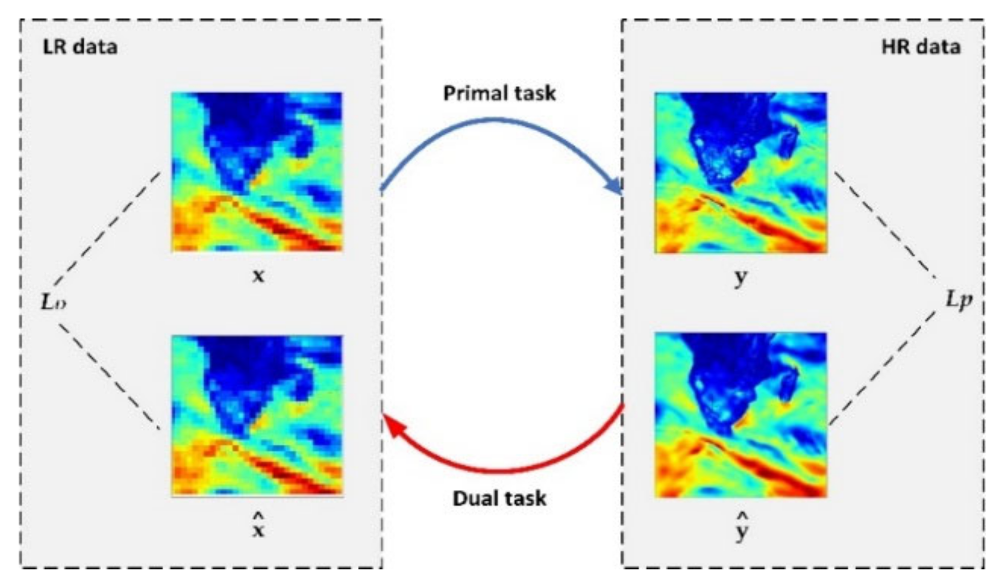
• In the dual learning scheme, a primal task to reconstruct HR images and a dual task to estimate the degradation kernels are simultaneously learned by minimizing the loss in a closed loop, thus yielding better performance. By integrating the dual learning scheme into the GAN structure as the generator, the downscaling performance is further improved by introducing an additional constraint to reduce the solution space. The model adaptation strategy of the proposed approach can improve the downscaling performance on the unpaired LR SSW.

The remainder of this paper is structured as follows. Section 2 presents the study area and sea surface data used. Section 3 gives the proposed downscaling approach, including the overview, data preprocessing module, the generator architecture based on dual learning scheme, the discriminator architecture, the loss function, and model training strategy. Section 4 gives the experimental configuration and results. Section 5 discusses the results from the aspects of the downscaling network, the capacity to unpaired SSW LR data, downscaling spatial resolution enhancement etc. Conclusions are drawn in Section 6.

2. Study Areas and Data

2.1. Study Areas

The offshore areas are closely related to human activities, and accurate mapping and understanding of SSW information are of great significance to social and economic activities. Therefore, the study areas in this paper include the East Coast of North America (ranging from 85°W to 45°W, 10°N to 50°N, hereinafter referred to as Region 1), and the North Indian Ocean (ranging from 55°E to 95°E, 15°S to 20°N, Region 2) as shown in Figure 1, where sufficient buoy observations are publicly available.

2.2. Sea Surface Wind Data

In this study, two categories of SSW data are used: (1) in situ buoy measurements from the National Data Buoy Center (NDBC) and the Research Moored Array for African-Asian-Australian Monsoon Analysis and Prediction (RAMA), and (2) SSW derived from the radiometer WindSat satellite observations as a case study. The proposed downscaling method is applied to the satellite observations, while the buoy measurements are used as ground truth for validation of SSW. The spatial coverage is depicted in Figure 1, and the time ranges from 2017 to 2019.

2.2.1. Buoy Measurements

In the regions of the East Coast of North America (Region 1), the buoy SSW measurements were collected from the NDBC (https://www.ndbc.noaa.gov/ (accessed on 3 February 2022)) of the National Oceanic and Atmospheric Administration (NOAA) in the form of standard meteorological data reported hourly. NDBC designs, develops, operates, and maintains a network of data collecting buoys and coastal stations. The standard meteorological data of NDBC buoy stations provide wind direction and wind speeds averaged over an eight-minute period for buoys at each hour [2]. In this study, 33 NDBC stations are used for Region 1, and the heights of wind measurements vary.

In the region of the North Indian Ocean (Region 2), the RAMA buoy data of 23 stations were obtained from Pacific Marine Environmental Laboratory’s global tropical moored buoy array (https://www.pmel.noaa.gov/tao/drupal/disdel/ (accessed on 3 February 2022)) [24]. RAMA is the tropical buoys array over the Indian Ocean deployed to measure various atmospheric and oceanic parameters and provide the surface winds at 4 m height [25].

In this study, we use the bulk algorithm COARE 4.0 algorithm (packages: https://cerform.readthedocs.io/en/latest/api/cerform.flux.html#module-cerform.flux.coare4 (accessed on 3 February 2022)) to calibrate the NDBC, and RAMA winds to neutral-equivalent winds at a standard 10 m reference height, which are comparable with the satellite observations wind products [26,27]. The COARE bulk algorithm iteratively solves equations involving the air–sea exchanges of momentum, heat, and water vapor to arrive at the wind speed profile in the lower atmospheric boundary layer [28].

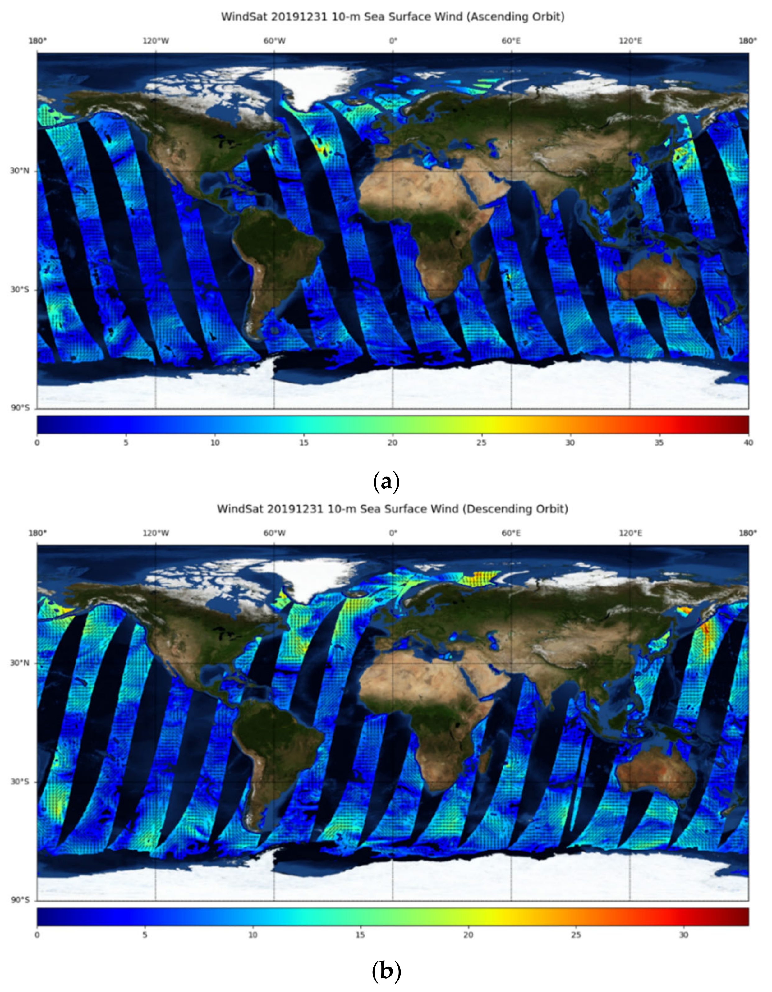
2.2.2. Satellite Observations

In this paper, we use the satellite SSW observations from WindSat as a typical case study for our downscaling. Compared with the traditional microwave radiometer, which can only obtain wind speed, WindSat is the first space-borne microwave full polarimetric radiometer launched in 2003 aboard the Coriolis satellite [29]. It was developed by the naval research laboratory (NRL) remote sensing division and the naval center for space technology for the U.S. Navy, and the national polar-orbiting operational environmental satellite system (NPOESS) integrated program office (IPO). WindSat further extracts the polarization information of the target and offers the capabilities to measure SSW vector [30]. Compared with scatterometer, the widely used active wind measurement instrument for SSW observation, the fully polarized microwave radiometer can obtain sea surface temperature (SST), cloud water, rain rate etc., simultaneously. Extensive validation of the wind vector from WindSat was conducted with buoy measurements, other satellite observations as well as numerical winds [31], and the WindSat SSW was widely used for decades [29,32,33]. In this study, we use the v7.0.1 daily WindSat SSW measurements under all weather conditions with a spatial resolution of 0.25° × 0.25° in the form of ascending and descending swaths, which are available from remote sensing systems (RSS) [34]. Figure 2 show a global 10 m SSW map from WindSat, taking 31 December 2019, as an example with both the ascending passes and the descending passes.

3. Methodology

3.1. Overview

The flowchart of the method presented in this paper is shown in Figure 3. The methodology involves three stages as follows, and more information is outlined in Section 3.2 and Section 3.3.

(a) Data preprocessing. The original SSW and the LR data generated by downsampling constitute a synthetic LR-HR paired dataset. The u and v wind components are extracted from the WindSat satellite SSW fields and normalized, which are taken as input channels of the downscaling network together with the corresponding mask channel.

(b) Downscaling model training and inferencing. In this paper, we put forward a novel spatial downscaling approach for satellite SSW from WindSat based on the generative adversarial network (GAN) and dual learning. A dual learning network to reconstruct the HR SSW is adopted as the generator, which performs downscaling, i.e., the super-resolution process, by mapping input coarse data to the associated finer data. The discriminator classifies the image patches as real (from the HR of the training set) or fake (from the generator). The network architecture of the discriminator is given in Section 3.3.3 in detail. In this work, we first trained a downscaling model with the synthetic LR-HR paired SSW and further performed the model adaptation by sampling both unpaired SSW (i.e., the 0.25° SSW as LR data) and synthetic paired SSW based on the dual learning scheme. The latter trained model is used to generate higher resolution results from the 0.25° SSW as LR input.

(c) Performance comparison and analysis. Typical reference methods include the cubic convolution interpolation, DeepSD, DRN, and adversarial DeepSD, as well as downscaling inference directly from the model trained with the synthetic paired SSW. The accuracy of downscaling results against buoy measurements adjusted to the height of 10m is validated and analyzed.

3.2. Data Preprocessing

The original WindSat satellite sea surface wind data from RSS are at the spatial resolution of 0.25° and contain wind speed w and wind direction θ (degrees oceanographic). For the proposed downscaling method in this paper, the ultimate goal of which is to obtain SSW with higher resolution than 0.25°, hence in the downscaling with unpaired SSW, in view of the downsampling kernel from the realistic HR SSW to the LR data is unknown, we selected and performed a downsampling method from the sets of the commonly used nearest, bilinear, and bicubic interpolation randomly to an input HR image to obtain the synthetic LR data (for instance, 2°), to better represent the unknown degradation. In this work, we adopted the SSW data in the form of u and v components and the mask as the input channels for the downscaling network. The u (zonal) and v (meridional) wind components can be transformed from the w and θ, as shown in Equations (1) and (2). The value in the mask is either 0 or 1, indicating whether the wind field at a pixel is null or not. Since the ranges of wind speed and wind direction are 0–50 m/s and 0–360°, respectively, the normalization operation was applied, as shown in Equations (3) and (4) before feeding into the network.

$$u=w\sin \theta$$

(1)

$$v=w\cos \theta$$

(2)

$$\mathrm{channel}\_1=\left(u+50\right)/100$$

(3)

$$\mathrm{channel}\_2=\left(v+50\right)/100$$

(4)

3.3. Downscaling Network Architecture

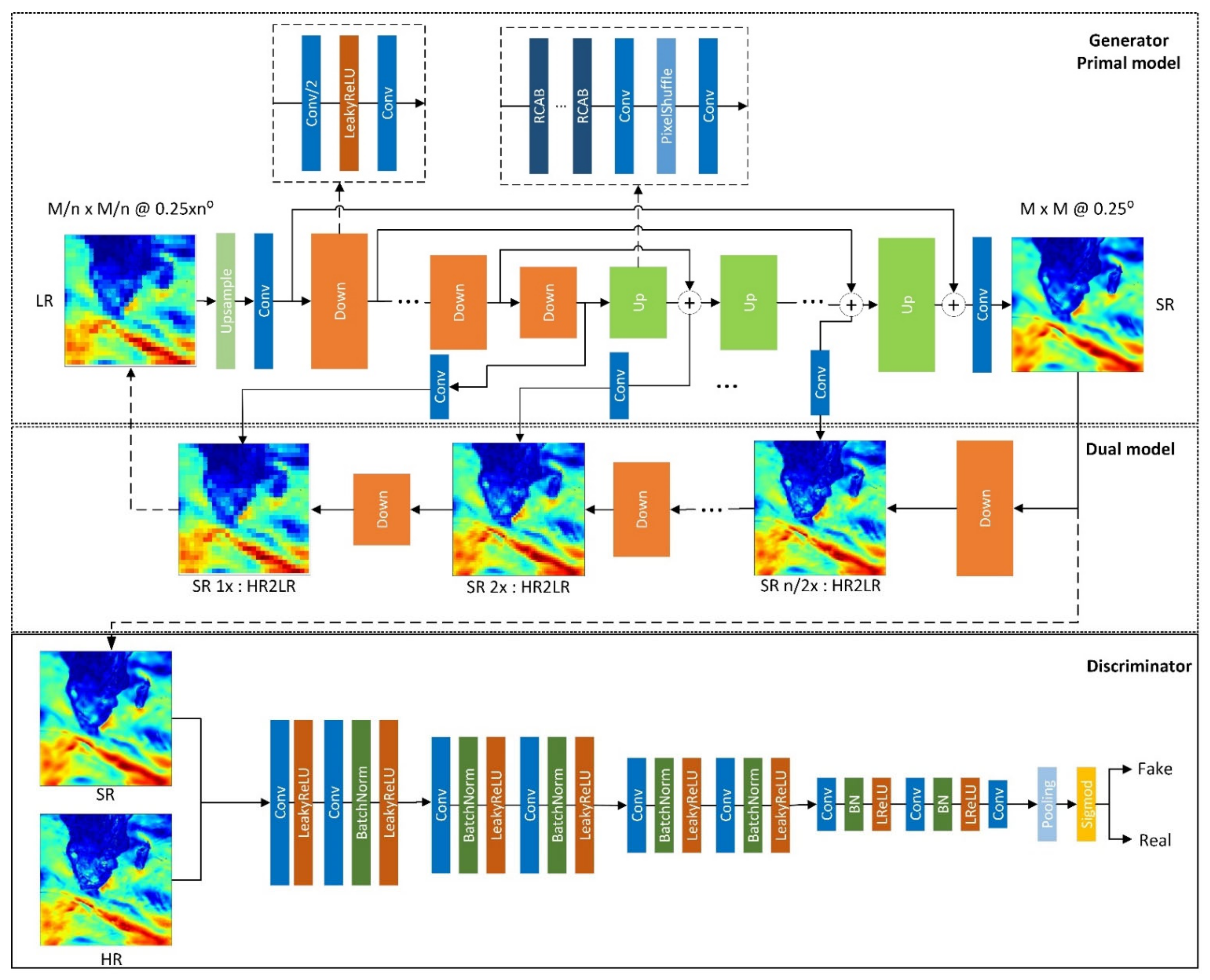
3.3.1. Generative Adversarial Network Structure

Generative Adversarial Network (GAN) [35] was originally inspired by the two-player zero-sum game, which is composed of two sub-networks, a generator that tries to generate data samples as real as possible, and a discriminator that tries to discriminate the fake samples and real ones. Its goal is to generate samples from the same distribution of existing data. GAN has attracted great attention and was intensively investigated in recent years due to its promising performance in generative tasks such as text/image-to-image translation and realistic image synthesis.

In our task of downscaling, the generator maps the LR images to super-resolved images, and the discriminator attempts to distinguish HR images from the super-resolved images. The overall framework, as illustrated in Figure 4, also consists of a generator network G and a discriminator network D, which will be described in Section 3.3.2 and Section 3.3.3. The generator network is designed with a state-of-the-art dual learning network, which is fed with LR SSW and outputs corresponding super-resolution SSW. The reconstructed super-resolution SSW and real high-resolution SSW are input into the discriminator network, which is a typical classification network. If the discriminator network recognizes the reconstructed one, it means the quality of the reconstructed SSW is unsatisfactory, and the loss will be fed to the generator network. During the adversarial training, the generator network can generate more realistic details of the wind field, and the discriminator network can grow the capability of finding the super-resolution images. This process will be repeated until the losses of both the generator and the discriminator reach a minimum.

3.3.2. Generator Based on Dual Learning

Although many deep neural networks are proposed for image super-resolution, most methods suffer from the following limitations: (a) Since an LR image may be down-sampled from infinite HR images, learning the mapping function from LR to HR images is an ill-posed issue, which makes it hard to learn a good solution in a large possible function space; (b) In real world applications, e.g., SSW downscaling in this study, the HR data is hard to collect and the paired LR-HR data may be unavailable. Most DL-based SR methods, which rely on the paired training data, often incur the adaptation issue and yield poor performance. In this context, dual learning provides a solution for super-resolution performance improvement.

The dual learning scheme involves two types of tasks, i.e., a primal task f: x → y and a dual task g: y → x. The original signals are mapped forward by $\widehat{y}$ = f(x) and backward by $\widehat{x}$ = g(y). Figure 5 show an illustration of this process, in which $x ϵ X$ are LR images and y $ϵ Y$ are HR images, and L_P and L_D are the primal regression loss and the dual regression loss, respectively. The primal mapping P to reconstruct HR images $\widehat{y}$ and the dual mapping D to estimate the down-sampling kernel and reconstruct LR images $\widehat{x}$ are simultaneously learned by minimizing the loss in a closed loop. The dual mapping learns the degradation kernel, and if the generated super-resolution SSW is closer to HR SSW, the reconstructed LR SSW is closer to the input LR SSW; thus the primal and dual models are improved together to achieve better performance [36].

In this paper, we construct the generator for SSW downscaling based on a state-of-the-art dual learning method for single image super-resolution, i.e., dual regression networks (DRN) proposed by Guo et al. in [37]. In DRN, they introduced a constraint on LR images to reduce the possible solution space, performed experiments of image super-resolution with 8×, and achieved superior performance.

The network architecture of generator to downscale SSW in this work is shown in the upper part of Figure 4. The network is built based on U-Net and contains a primal network and a dual network. The primal network is composed of n down blocks and n up blocks, where n refers to the log₂(s), in which s denotes the scale factor. In this work, according to the downscaling resolution requirements, we set s as 16, which results in higher resolution gridded SSW (for instance, 0.015625° for 16×). This implies that n is 4. A basic block is composed of a residual channel attention block (RCAB) [38] to improve the capacity. Besides, a simple dual network with two convolution layers and a LeakyReLU activation layer is designed to down-sample LR images. The detailed structures and parameters of down, up, and dual blocks are listed in

Table 1. The network architecture configuration of generator based on dual learning scheme. The convolutional layer is represented as Conv (kernel_size, stride, padding), and h and w are the height and width of the input LR images. B is the number of RCABs, and F is the number of base feature channels.

Model	Model Details	Input Shape	Output Shape
Upsample	Upsample(16)	(3, h, w)	(3, 16h, 16w)
Head	Conv(3, 1, 1)	(3, 16h, 16w)	(1F, 16h, 16w)
Down 1	Conv(3, 2, 1)-LeakyRelu-Conv(3, 1, 1)	(1F, 16h, 16w)	(2F, 8h, 8w)
Down 2	Conv(3, 2, 1)-LeakyRelu-Conv(3, 1, 1)	(2F, 8h, 8w)	(4F, 4h, 4w)
Down 3	Conv(3, 2, 1)-LeakyRelu-Conv(3, 1, 1)	(4F, 4h, 4w)	(8F, 2h, 2w)
Down 4	Conv(3, 2, 1)-LeakyRelu-Conv(3, 1, 1)	(8F, 2h, 2w)	(16F, 1h, 1w)
Up 1	B RCAs	(16F, 1h, 1w)	(16F, 1h, 1w)
	Conv(3,1,1)-PixelShuffle(2)	(16F, 1h, 1w)	(16F, 2h, 2w)
	Conv(1, 1, 0)	(16F, 2h, 2w)	(8F, 2h, 2w)
Concatenation 1	Concatenate the output of Down 3 and Up 1	(8F, 2h, 2w) ⊕ (8F, 2h, 2w)	(16F, 2h, 2w)
Up 2	B RCAs	(16F, 2h, 2w)	(16F, 2h, 2w)
	Conv(3,1,1)-PixelShuffle(2)	(16F, 2h, 2w)	(16F, 4h, 4w)
	Conv(1, 1, 0)	(16F, 4h, 4w)	(4F, 4h, 4w)
Concatenation 2	Concatenate the output of Down 2 and Up 2	(4F, 4h, 4w) ⊕ (4F, 4h, 4w)	(8F, 4h, 4w)
Up 3	B RCAs	(8F, 4h, 4w)	(8F, 4h, 4w)
	Conv(3,1,1)-PixelShuffle(2)	(8F, 4h, 4w)	(8F, 8h, 8w)
	Conv(1, 1, 0)	(8F, 8h, 8w)	(2F, 8h, 8w)
Concatenation 3	Concatenate the output of Down 1 and Up 3	(2F, 8h, 8w) ⊕ (2F, 8h, 8w)	(4F, 8h, 8w)
Up 4	B RCAs	(4F, 8h, 8w)	(4F, 8h, 8w)
	Conv(3,1,1)-PixelShuffle(2)	(4F, 8h, 8w)	(4F, 16h, 16w)
	Conv(1, 1, 0)	(4F, 16h, 16w)	(1F, 16h, 16w)
Concatenation 4	Concatenate the output of Head and Up 4	(1F,16h, 16w) ⊕ (1F, 16h, 16w)	(2F, 16h, 16w)
Tail 0	Conv(3, 1, 1)	(16F, 1h, 1w)	(3, 1h, 1w)
Tail 1	Conv(3, 1, 1)	(16F, 2h, 2w)	(3, 2h, 2w)
Tail 2	Conv(3, 1, 1)	(8F, 4h, 4w)	(3, 4h, 4w)
Tail 3	Conv(3, 1, 1)	(4F, 8h, 8w)	(3, 8h, 8w)
Tail 4	Conv(3, 1, 1)	(2F, 16h, 16w)	(3, 16h, 16w)
Dual 1	Conv(3, 2, 1)-LeakyRelu-Conv(3, 1, 1)	(3, 16h, 16w)	(3, 8h, 8w)
Dual 2	Conv(3, 2, 1)-LeakyRelu-Conv(3, 1, 1)	(3, 8h, 8w)	(3, 4h, 4w)
Dual 3	Conv(3, 2, 1)-LeakyRelu-Conv(3, 1, 1)	(3, 4h, 4w)	(3, 2h, 2w)
Dual 4	Conv(3, 2, 1)-LeakyRelu-Conv(3, 1, 1)	(3, 2h, 2w)	(3, 1h, 1w)

.

The detailed configuration for the generator network, taking the downscaling 16× as an example, is provided in Table 1. The convolutional layer is represented as Conv (kernel_size, stride, padding), and h and w are the height and width of the input LR images. Let B be the number of RCABs and F be the number of base feature channels. For a 16× downscaling generator network, we set B = 36 and F = 10. The reduction ratio is set as r = 16 in all RCABs, and the negative slope is 0.2 for all LeakyReLU.

3.3.3. Discriminator Architecture

Our discriminator is a typical classification network, which consists of four convolutional blocks and a tail layer, following the idea of a representative GAN-based super-resolution network, e.g., SRGAN [39], SRFeat [40], and DSCSRGAN [41]. Each convolutional block is a cascaded sequence of convolutional layer activation operations. The parameters of convolutional layers in each block were adjusted based on experiments. The size of kernel, stride, and padding of convolutional layers of each block is 3, 1, 1 for the first one, and 4, 2, 1 for the second. Moreover, we append another convolutional layer to narrow down the dimensions of the features. The tail layer is composed of adaptive average pooling and Sigmoid operation, which can ensure that the output of the discriminator with various dimensions of input is a probability value. The size of the input image is 3 × 16H × 16W, where H and W are the height and width factors. Detailed information on the network architecture is given in

Table 2. The network architecture configuration of the discriminator.

Model	Model Details	Input Shape	Output Shape
Block 1	Conv(3, 1, 1)	(3, 16H, 16W)	(64, 16H, 16W)
	LeakyReLU	(64, 16H, 16W)	(64, 16H, 16W)
	Conv(4, 2, 1)	(64, 8H, 8W)	(64, 8H, 8W)
	BatchNorm-LeakyReLU	(64, 8H, 8W)	(64, 8H, 8W)
Block 2	Conv(3, 1, 1)	(64, 8H, W)	(128, 8H, 8W)
	BatchNorm-LeakyReLU	(128, 8H, 8W)	(128, 8H, 8W)
	Conv(4, 2, 1)	(128, 8H, 8W)	(128, 4H, 4W)
	BatchNorm-LeakyReLU	(128, 4H, 78)	(128, 4H, 4W)
Block 3	Conv(3, 1, 1)	(128, 4H, 4W)	(256, 4H, 4W)
	BatchNorm-LeakyReLU	(256, 4H, 4W)	(256, 4H, 4W)
	Conv(4, 2, 1)	(256, 4H, 4W)	(256, 2H, 2W)
	BatchNorm-LeakyReLU	(256, 2H, 2W)	(256, 2H, 2W)
Block 4	Conv(3, 1, 1)	(256, 2H, 2W)	(512, 2H, 2W)
	BatchNorm-LeakyReLU	(512, 2H, 2W)	(512, 2H, 2W)
	Conv(4, 2,1)	(512, 2H, 2W)	(512, H, W)
	BatchNorm-LeakyReLU	(512, H, W)	(512, H, W)
	Conv(4, 1, 1)	(512, H, W)	(1, H-1, W-1)
Tail	AdaptiveAvgPool-Sigmoid	(1, H-1, W-1)	(1, 1)

.

3.3.4. Loss Function and Model Training

In this section, we depict the loss functions of the generator network and the discriminator network, respectively. Given that y is the high-resolution image and x is the input low-resolution image, we define the loss function of the generator network from three aspects, as in Equations (5)–(8). The first one is the content loss ${\mathcal{L}}_{\mathrm{content}}$ that is to estimate the content difference between the super-resolution image and the real high-resolution image, which is measured by their pixel-wise L1 distance. The second is the dual regression loss ${\mathcal{L}}_{\mathrm{dual}}$ we used for unpaired data in Section 3.3.2, which is also formulated by L1 distance. We also use the adversarial loss ${\mathcal{L}}_{\mathrm{Aadversarial}}$ from the discriminator output in order to measure the degree of super-resolution image quality that can fool the discriminator. The coefficients ${\lambda }_1$ and ${\lambda }_2$ in Equation (5) are used to balance the magnitudes of its components. In this paper, we set ${\lambda }_1$ = 0.1 and ${\lambda }_2=0.01$. In Equation (5), 1S_P(x) is an indicator function. It equals 1 when x belongs to the paired samples, and otherwise, the function equals 0. The discriminator is expected to output 1 for the real high-resolution images and 0 for the super-resolution images from the generator network. Therefore, a commonly cross-entropy loss ${\mathcal{L}}_{\mathrm{D}}$ is used, as in Equation (9). The pseudo-code of the training process is given in Algorithm 1, in which ${\lambda }_U$ is the data ratio of unpaired data samples. The training of paired data can also be given uniformly in Algorithm 1 when setting ${\lambda }_U=0$.

$${\mathcal{L}}_{\mathrm{G}}\left(x,y\right)=1S_p\left(x\right)\left({\mathcal{L}}_{\mathrm{content}}\left(x,y\right)+{\lambda }_2{\mathcal{L}}_{\mathrm{Aadversarial}}\left(x,y\right)\right)+{\lambda }_1{\mathcal{L}}_{\mathrm{dual}}\left(\mathrm{G}\left(x\right),y\right)$$

(5)

$${\mathcal{L}}_{\mathrm{content}}\left(x,y\right)=\left|y-\mathrm{G}\left(x\right)\right|$$

(6)

$${\mathcal{L}}_{dual}\left(G\left(x\right),y\right)=\left|x-D_{ual}\left(G\left(x\right)\right)\right|$$

(7)

$${\mathcal{L}}_{Aadversarial}\left(x,y\right)=-log{D}_{is}\left(G\left(x\right)\right)$$

(8)

$${\mathcal{L}}_{Dis}\left(x,y\right)=-log{D}_{is}\left(y\right)-log\left(1-D_{is}\left(G\left(x\right)\right)\right)$$

(9)

Algorithm 1: Algorithm for Higher Resolution with Unpaired Data.

1 Input 1: The wind field data (0.25°) as LR: Unpaired data {yi};

2 Input 2: The synthetic data as LR (2°) and HR (0.25°): Paired data {xi, yi};

3 Load the pretrained models: generator (G), dual regression (Dual) and discriminator (Dis);

4 Whilenot convergentdo

5   UnpairedTraining = True if random(0, 1) < λU, vice versa;

6   ifnot UnpairedTrainingthen

7   //Update the Dis model

8   Update Dis by minimizing the objective: $\sum L_{Dis}\left(x_i, y_i\right)$;

9   //Update the G model

10    Update G by minimizing the objective: $\sum L_{content}\left(x_i, y_i\right)+{\mathsf{\lambda }}_1{L}_{dual}\left(G\left(x_i\right), x_i\right)+{\mathsf{\lambda }}_2{L}_{adversarial}\left(x_i, y_i\right)$;

11    //Update the Dual model

12    Update Dual by minimizing the objective: $\sum {\mathsf{\lambda }}_1{L}_{dual}\left(G\left(x_i\right), x_i\right)$;

13  else

14    //Update the Dual model

15    Update Dual by minimizing the objective:$\sum {\mathsf{\lambda }}_1{L}_{dual}\left(G\left(y_i\right), y_i\right)$;

16  end

17 end

4. Experiments and Results

4.1. Evaluation Metrics

To evaluate the proposed downscaling method, we adopt two sets of metrics in this paper. The first set validates the downscaling SSW results with buoy measurements using root mean square error (RMSE) and coefficient of determination, i.e., R-Square ($R^2$). Their definitions are formulated in Equations (10) and (11). $O_i$ and $Y_i$ represent the observation and the downscaling value of the i-th record, respectively. N is the number of matched SSW records. $\overline{O}$ is the mean of the observed data. RMSE is the standard deviation of the residuals. The lower this metric is, the better the performance, and vice versa. $R^2$ shows the variance of the downscaling estimation from the measured data.

$$RMSE=\sqrt{\frac{1}{N}{\displaystyle \sum }_{i=1}^N{\left(O_i-Y_i\right)}^2}$$

(10)

$$R^2=1-{\displaystyle \sum }_{i=1}^N{\left(O_i-Y_i\right)}^2/{\displaystyle \sum }_{i=1}^N{\left(O_i-\overline{O}\right)}^2$$

(11)

The second set of metrics measures the downscaling reconstruction quality, and the peak signal-to-noise ratio (PSNR) and structural similarity(SSIM) are used. PSNR is a commonly used reconstruction quality metric of lossy transformation such as image compression and image inpainting. In the scenario of super-resolution, given the ground truth image I with M pixels and the reconstructed image $\widehat{I}$, PSNR is defined as Equation (12), where $MA{X}_I$ is the maximum pixel value of the image, such as 255 for 8-bit images. SSIM is a metric that measures the structural similarity of images from the aspects of luminance, contrast, and structure. The formulation are given in Equations (13)–(16). The luminance $\mu$ and contrast $\sigma$ are estimated with the mean and standard deviation of the image intensity, ${\sigma }_{I\widehat{I}}$ is the covariance of image $I$ and $\widehat{I}$. Constants c₁, c₂, and c₃ are for stability. Control parameters α, β, and γ are for adjusting the relative importance, here are set as 1 [42].

$$\mathrm{PSNR}=10⬝{\log }_{10}\left(\frac{MA{X}_I{}^2}{\frac{1}{M}{{\displaystyle \sum }}_{i=1}^M{\left(I\left(i\right)-\widehat{I}\left(i\right)\right)}^2}\right)$$

(12)

$$l\left(I,\widehat{I}\right)=\frac{2{\mu }_I{\mu }_{\widehat{I}}+c_1}{{\mu }_I^2+{\mu }_{\widehat{I}}^2+c_1}, c_1={\left(k_{1}MA{X}_I\right)}^2$$

(13)

$$c\left(I,\widehat{I}\right)=\frac{2{\sigma }_I{\sigma }_{\widehat{I}}+c_2}{{\sigma }_I^2+{\sigma }_{\widehat{I}}^2+c_2}, c_2={\left(k_{2}MA{X}_I\right)}^2$$

(14)

$$\mathrm{s}\left(I,\widehat{I}\right)=\frac{{\sigma }_{I\widehat{I}}+c_3}{{\sigma }_I{\sigma }_{\widehat{I}}+c_3}, c_3=c_2/2$$

(15)

$$SSIM\left(I,\widehat{I}\right)={\left[l\left(I,\widehat{I}\right)\right]}^{\alpha }⬝{\left[c\left(I,\widehat{I}\right)\right]}^{\beta }⬝{\left[s\left(I,\widehat{I}\right)\right]}^{\gamma }=\frac{\left(2{\mu }_I{\mu }_{\widehat{I}}+c_1\right)\left(2{\sigma }_{I\widehat{I}}+c_2\right)}{\left({\mu }_I^2+{\mu }_{\widehat{I}}^2+c_1\right)\left({\sigma }_I^2+{\sigma }_{\widehat{I}}^2+c_2\right)}$$

(16)

4.2. Reference Methods

In this paper, we adopt the following typical methods for performance comparison:

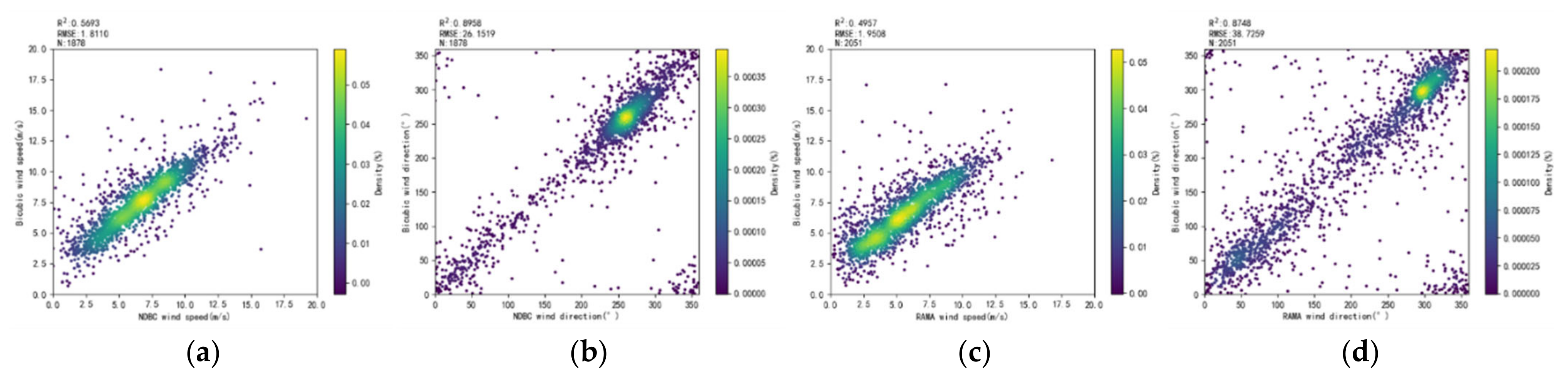
• Cubic convolution interpolation [43] is a classical technique for resampling discrete data, the accuracy of which is between that of linear interpolation and that of cubic splines with the appropriate boundary conditions and constraints on the interpolation kernel. We adopted the cubic convolution interpolation as one of the reference methods since it is widely used to validate the performance of super-resolution.
• DeepSD [20] is an augmented stacked super-resolution convolutional neural network framework for statistical downscaling of climate variables and earth system model simulations proposed by Vandal et al. in 2017 and has achieved a downscaling factor of 8x. It is the first research of climate downscaling by the deep learning-based super-resolution technique to the best of our knowledge, and has provided NASA Earth Exchange (NEX) an alternative to generate the downscaled products at high resolutions, thus being selected as a method for comparison.
• Adversarial DeepSD is a reference method to evaluate the effectiveness of GAN, which takes DeepSD as the generator and the same discriminator network as the proposed method in this paper.
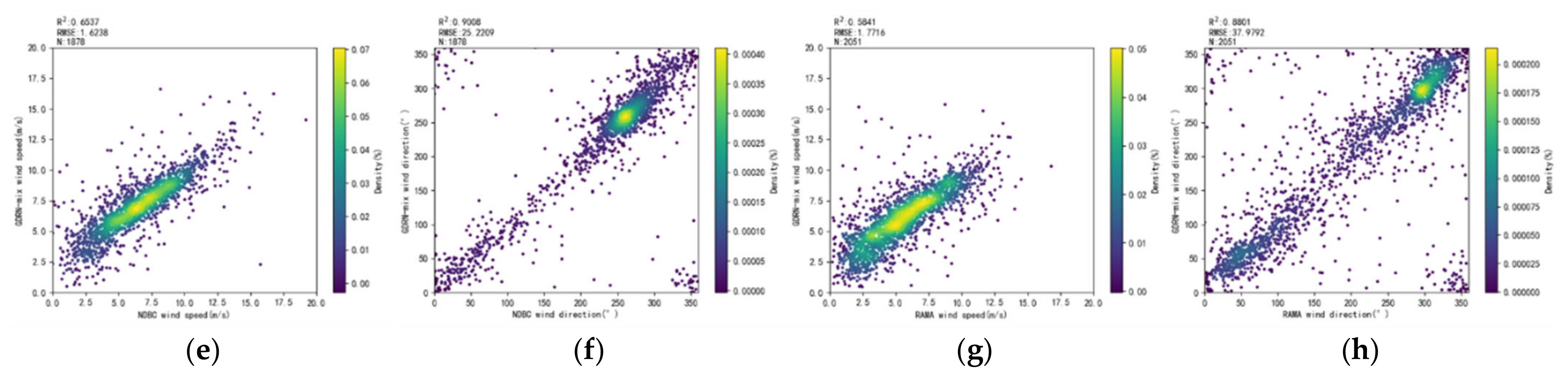
• Dual regression networks [37] is a dual regression scheme proposed by Guo et al. in 2020 by introducing an additional constraint on LR data to reduce the possible function space. It not only learns the mapping from LR to HR images but also learns the extra mapping that estimates the down-sampling kernel for reconstructing LR images, thus forming a closed loop for better performance. DRN is the base network for the presented SSW downscaling approach in this paper, which is also used for performance comparison.

4.3. Experimental Setup

The experiments are performed on a server including two Intel Xeon E5-2680 v4 CPUs, each running at a base frequency of 2.40 GHz with 14 cores and 64 GB of random access memory. The server is equipped with an NVIDIA RTX 3090 GPU, which combines 10,496 compute unified device architecture (CUDA) cores based on Ampere 8 nm architecture and has 24 GB of GDDR6X memory that runs at 19.5 Gbps. The system runs Ubuntu 20.04.3 LTS with Python3.8 and PyTorch 1.9.1.

The presented method is applied to WindSat satellite SSW data. We collected 3 years of WindSat daily SSW ranging from 2017 to 2019 from RSS. A daily SSW contains two orbits of image data, and therefore we obtained 2172 global SSW image data in total. We randomly assign 80% as training data (1738 images) and 20% as test data (434 images). During the training, we randomly slice the global data into the n × n patch, where the n is set according to the size of GPU memory. In our cases, n is set as 384. The models trained with the training dataset are used to estimate downscaling results globally and validated with buoy measurements for the study area Region 1 and Region 2, as shown in Figure 1.

In this paper, the following experiments have been conducted to validate and analyze the performance of the presented SSW downscaling approach.

• Experiment 1: The synthetic experiments on the constructed paired LR and HR SSW. Since it is common that the downscaling evaluation suffers from a lack of ground truth, synthetic experiments are usually conducted by upscaling higher spatial resolution products, which are then taken as input, and comparing the downscaled results with original products [44]. In this paper, we first obtain the LR SSW from the original 0.25° SSW with the commonly used bicubic interpolation. Models, including DeepSD, DRN, adversarial DeepSD, and the proposed network based on GAN and dual learning, are trained, respectively, with the LR-HR training dataset, and the downscaling results from the trained models are validated on the test dataset with the evaluation metrics including RMSE and R², as well as PSNR and SSIM.
• Experiment 2: Downscaling experiments to generate higher resolution SSW data without HR ground truth. In real scenes, HR ground truths are usually unavailable. Therefore, we adopted the 0.25° SSW as LR data to form an unpaired dataset and applied the adaptation for our model based on GAN and dual learning, as shown in Algorithm 1 in Section 3.3.4, together with the synthetic LR-HR dataset. In this experiment, we generated SSW at 0.03125° (a downscaling factor of 8×) with the default configuration of basic blocks. Due to the lack of the HR SSW images, we only present the RMSE and R² against buoy measurements for the downscaling accuracy validation and comparison.
• Experiment 3: The downscaling capacity to generate higher resolution. Based on experiment 2, we further increased the basic blocks in the generator of the network to achieve a downscaling factor of 16× (0.015625° spatial resolution) with comparable accuracy.

4.4. Downscaling Results

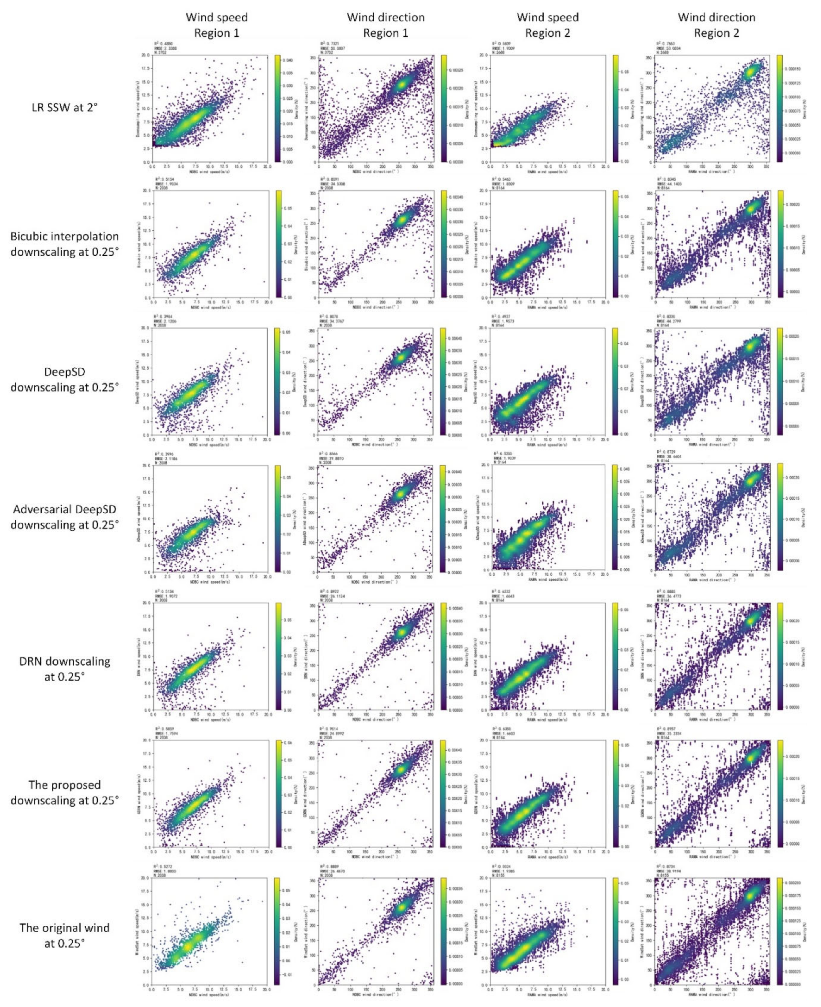
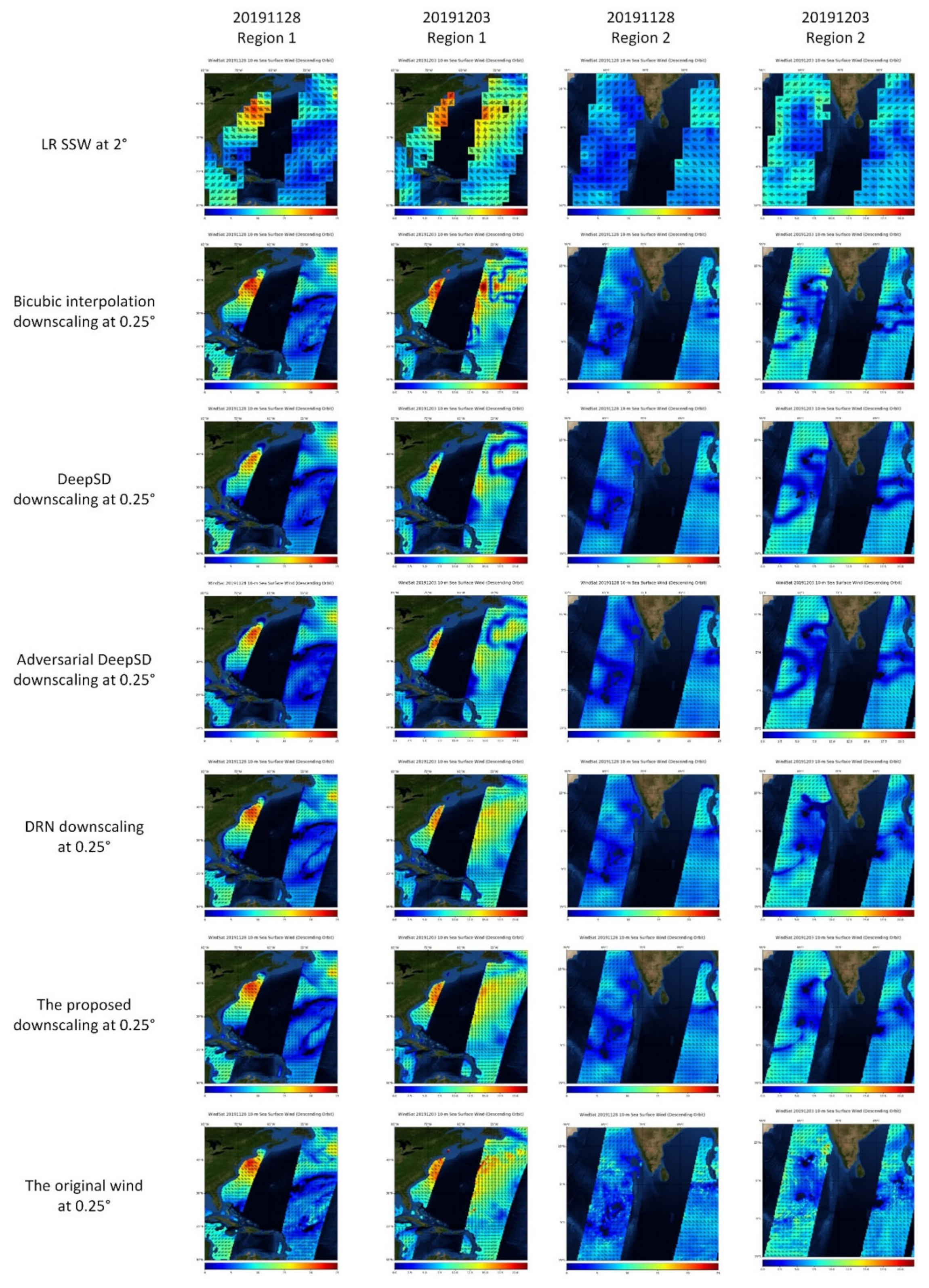
4.4.1. Results on Synthetic LR-HR SSW

We report the accuracy validation results in terms of RMSE and R² for the downscaling SSW with buoy measurements in

Table 3. Accuracy validation of sea surface wind downscaling with buoy measurements in terms of RMSE and R² on the test dataset for the study areas in Figure 1.

Type	Resolution	Method	Component	Region 1		Region 2
				RMSE	R2	RMSE	R2
Original HR	0.25°	Original HR	Direction	26.49	0.89	38.92	0.87
			Speed	1.88	0.53	1.94	0.50
LR	2°	Bicubic downsample 8×	Direction	50.08	0.73	56.38	0.74
			Speed	2.34	0.49	1.91	0.60
Downscaling HR	0.25°	Bicubic interpolation	Direction	34.53	0.81	44.14	0.83
			Speed	1.90	0.52	1.85	0.55
		DeepSD	Direction	34.38	0.81	44.28	0.83
			Speed	2.12	0.40	1.96	0.49
		Adversarial DeepSD	Direction	29.88	0.86	38.66	0.87
			Speed	2.12	0.40	1.90	0.52
		DRN	Direction	26.11	0.89	36.48	0.89
			Speed	1.91	0.51	1.66	0.63
		Proposed method	Direction	24.90	0.90	35.23	0.90
			Speed	1.76	0.59	1.66	0.63

and the reconstruction performance in terms of PSNR and SSIM in

Table 4. Downscaling reconstruction quality of sea surface wind in terms of PSNR and SSIM for the study areas in Figure 1.

Method	PSNR	SSIM
Bicubic interpolation	38.3350	0.9726
DeepSD	36.7467	0.9508
Adversarial DeepSD	36.6965	0.9570
DRN	39.4307	0.9771
Proposed method	39.9648	0.9805

for the study areas as shown in Figure 1. The corresponding validation scatter plots are given in Figure 6, where from left to right are for wind speed and wind direction in Region 1 and Region 2, and from top to bottom are for the LR SSW at 2°, downscaling SSW based on bicubic interpolation, DeepSD, DRN, adversarial DeepSD, the proposed method, and ground truth HR at 0.25°. Figure 7 depict the visualization images of SSW, taking 28 November 2019 and 3 December 2019 as examples, for Region 1 and Region 2, respectively. It can be noted from Table 3 and Figure 6 that our proposed downscaling method based on GAN and dual learning results in the highest accuracy and significantly outperforms the other downscaling methods with respect to the typically used metrics RMSE and R². It achieves the lowest RMSE of 24.90° and 1.76 m/s, 35.23° and 1.66 m/s, as well as the highest R² of 0.90 and 0.59, 0.90 and 0.63 in Region 1 and Region 2 for wind direction and wind speed, respectively. Table 4 show that our proposed method results in higher reconstruction quality with PSNR of 39.96 and SSIM 0.98. The higher these two values, the less distortion in the images compared with ground truth. From Figure 7, it can be seen that the bicubic interpolation, DeepSD, and adversarial DeepSD downscaling results contain significant inconsistencies compared with the ground truth in the last row (for instance, the upper right corner in the second column images, the middle left in the fourth column images). The downscaling results are the most similar to the ground truth; however, they are still relatively smooth and contain less texture detail.

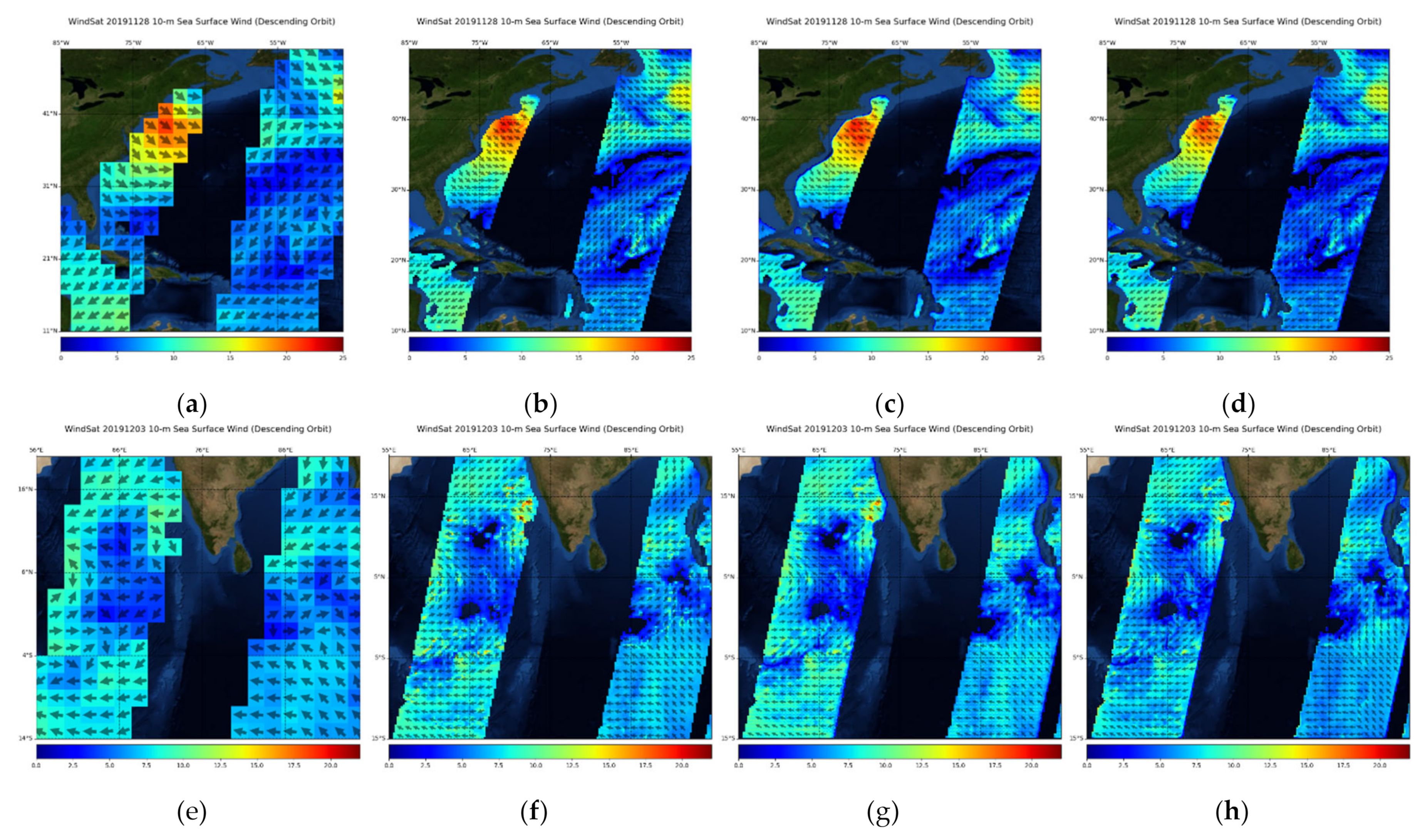
4.4.2. Results on LR SSW

In Section 4.4.1, we present the downscaling results on the synthetic LR-HR data, i.e., the original SSW are used as HR ground truth to validate our proposed method, and the spatial resolution of downscaling SSW corresponds to the original SSW of 0.25°. In this section, we take the 0.25° SSW as LR data and perform the model adaptation by sampling both unpaired SSW and synthetic paired SSW according to Algorithm 1 in Section 3.3.4.

Table 5. Accuracy comparison of sea surface wind downscaling to 8× at 0.03125°, to 16× at 0.015625° with buoy measurements.

Type	Resolution	Method	Component	Region 1		Region 2
				RMSE	R2	RMSE	R2
LR Input	0.25°	Original data	Direction	26.49	0.89	38.92	0.87
			Speed	1.88	0.53	1.94	0.50
Downscaling HR	0.25°/8 = 0.03125°	Bicubic interpolation	Direction	26.07	0.90	38.71	0.88
			Speed	1.82	0.57	1.96	0.49
		DeepSD	Direction	29.44	0.87	42.48	0.85
			Speed	2.21	0.36	2.16	0.38
		Adversarial DeepSD	Direction	32.28	0.84	45.26	0.83
			Speed	2.16	0.39	2.24	0.34
		DRN	Direction	31.01	0.85	44.24	0.84
			Speed	2.09	0.43	2.16	0.38
		Proposed model inference	Direction	33.24	0.83	45.58	0.83
			Speed	2.08	0.43	2.15	0.39
		Proposed model adaptation	Direction	25.19	0.90	37.63	0.88
			Speed	1.78	0.58	1.75	0.60
	0.25°/16 = 0.015625°	Bicubic interpolation	Direction	26.15	0.90	38.73	0.87
			Speed	1.81	0.57	1.95	0.50
		Proposed model adaptation	Direction	25.22	0.90	37.98	0.88
			Speed	1.62	0.65	1.77	0.58

compare the accuracy for SSW at different spatial resolutions. For the SSW at 0.03125° (downscaling 8×), our proposed method by further applying model adaptation outperforms the other downscaling methods (including the direct inference using the proposed method however trained with synthetic LR-HR SSW in Section 4.4.1) with the lowest RMSE of 25.19° and 1.78 m/s in Region 1, 37.63° and 1.75 m/s in Region 2. The corresponding R² is also the highest. Figure 8 give their specific validation scatter plots with buoy measurements for each method. For the SSW at 0.015625° (downscaling 16×), we only list the validation metrics for the bicubic interpolation and our proposed model adaptation on the unpaired LR SSW, since DeepSD can only provide 8× downscaling results and the 8x downscaling results have shown that the proposed model adaptation is obviously superior to the baseline DRN and direct model inference. Our proposed method also achieves the highest accuracy for the 16× SSW downscaling, and the specific scatter plots are shown in Figure 9. due to the lack of higher-resolution SSW ground truth for 8× and 16× downscaling, the PSNR and SSIM metrics are not provided. Besides, instead of presenting the visualization images of SSW of each method, in Figure 10, we show SSW at different spatial resolutions, i.e., 2°, 0.25°, 0.03125°, and 0.015625° in Region 1, taking 28 November 2019, as an example, and in Region 2 taking 3 December 2019, as an example. As can be seen in Figure 10, the higher resolution SSW displays more details.

5. Discussion

5.1. Downscaling Performance

In recent years, DL-based single-image super-resolution techniques were exploited for climate downscaling due to the similarity between single-image super-resolution tasks and statistical downscaling tasks, as well as the superior ability of DL to learn complex nonlinear feature representations. Therefore, in this paper, we present a spatial downscaling approach for satellite SSW based on GANs and dual learning scheme, taking WindSat as an example to generate higher spatial resolution SSW for regional or local studies. In Section 4.4, we demonstrate the downscaling results and comparison with reference methods, including both the traditional bicubic interpolation and the DL-based DeepSD, adversarial DeepSD, and DRN.

The results in Table 3 show the effectiveness of our proposed method based on GAN and dual learning with synthetic LR-HR SSW in terms of accuracy validation. Specifically, as the baseline generator, DRN achieved better downscaling accuracy performance compared with DeepSD. For example, in Region 2, DRN obtains an RMSE decrease of 7.66° and 0.19 m/s (−0.14° and −0.11 m/s for DeepSD), and an R² increase of 0.06 and 0.08 (0 and −0.06 for DeepSD) for wind direction and wind speed, respectively, taking the bicubic interpolation as a starting point. This implies the effectiveness of dual learning by introducing an additional constraint to reduce the solution space. The integration of GAN yields better performance for DeepSD and DRN. However, the performance improvement brought by GAN is smaller than that of DRN for the proposed method.

As revealed in Table 3, Table 4 and Table 5, the performance of DL-based methods, e.g., DeepSD, does not always outperform traditional methods such as the bicubic interpolation. For instance, DeepSD and Adversarial DeepSD show worse PSNR, as shown in Table 4. This could be due to the fact that DeepSD applies the stacked SRCNN [45], a simple CNN, to learn the mapping from LR to HR data. Its capability of feature extraction and nonlinear mapping is limited, which also depends on the data. DeepSD was proposed to downscale precipitation with the assistance of auxiliary elevation data [20]. However, in this work, we downscale SSW that contain large areas missing value grids between orbits or on land. These two tasks are similar but differences in the distribution of values and space exist. Therefore, the straightforward application of existing DL-based methods such as DeepSD may lead to performance degradation, and some adjustments such as network architecture are required for performance improvement.

Besides, the comparison results in Table 5 imply that mapping learned from a paired LR-HR SSW is not always suitable for the downscaling for higher resolutions. Our proposed method adopts a model adaptation training strategy by making use of both paired LR-HR SSW synthetic data and unpaired LR SSW data, which has been proved effective by experiments in Section 4.4.2.

5.2. Computational Efficiency

In addition to the accuracy and reconstruction quality of downscaling, computational efficiency is also a major concern in practical scenarios. In this paper, we adopted the widely used metrics of floating-point operations (FLOPs), parameters, and execution time to evaluate the efficiency performance [46,47,48]. We list the corresponding metrics of parameters and FLOPs in

Table 6. The parameters and FLOPs of the (primal) model during model inference.

Resolution	Method	Parameters	FLOPs
2° → 0.25° 0.25° → 0.03125° (8× downscaling)	Bicubic interpolation	0	102.4 K
	DeepSD	207,825	16.4 G
	Adversarial DeepSD
	DRN	10,000,772	63.57 G
	Proposed method
0.25° → 0.015625° (16× downscaling)	Bicubic interpolation	0	409.6 K
	Proposed model adaptation	41,071,601	367.02 G

and

Table 7. The parameters and FLOPs of the dual model and discriminator for dual learning/GAN-based methods.

Model	Parameters	FLOPs
Dual model	540 × n	220 × n K
Discriminator	7,134,401	187.42 M

and execution time in

Table 8. The execution time of the (primal) model during model inference.

Resolution	Method	Time (seconds/item)
2° → 0.25° 8× downscaling input size of 3 × 180 × 90	Bicubic interpolation	1.29
	DeepSD	1.31
	Adversarial DeepSD
	DRN	1.38
	Proposed method
0.25° → 0.03125° 8x downscaling input size of 3 × 160 × 300	Bicubic interpolation	1.03
	DeepSD	1.00
	Adversarial DeepSD
	DRN	1.19
	Proposed model inference
	Proposed model adaptation
0.25° → 0.015625° 16× downscaling input size of 3 × 160 × 300	Bicubic interpolation	3.24
	Proposed model adaptation	5.02

. It should be noted that only the primal model in the generator is used during downscaling, i.e., model inference after model training. Therefore, the measurements of the GAN-based methods, i.e., Adversarial DeepSD and the proposed method with GAN and dual learning, are equal to those of their generator (DeepSD and DRN), as shown in Table 6 and Table 8. The model parameters and FLOPs of the rest network, i.e., the dual model and discriminator that are not used during the model inference stage for the dual learning or GAN-based methods, are given in Table 7, where n refers to the logarithm to base 2 of the scale factor.

For the parameter size, DeepSD is a relatively simple network and has the capability of 8x downscaling with parameters of 207,825. The primal model in the generator of our network is a deeper network, and its parameter size is about 48.12× that of DeepSD with the same downscaling scale. When raising the downscaling scale, e.g., to 16×, basic blocks of the primal network are added, which leads to an increase in the parameter size. Compared with the primal model, the dual model and discriminator contain fewer parameters, as shown in Table 7.

The FLOPs were measured with an input with fixed dimensions at (3, 40, 40) for a fair comparison. The proposed method has higher FLOPs compared with the reference methods, and the FLOPs of the primal model account for a high proportion of the entire model. The FLOPs increase with the downscaling scale increasing.

When measuring the practical execution time in Table 8, global SSW (input size of 3 × 180 × 90) for the 8× downscaling (2° → 0.25°) and regional SSW (input size of 3 × 160 × 160 for region 1, and 3 × 160 × 140 for region 2) for the 8× downscaling (0.25° → 0.03125°) and 16× downscaling (0.25° → 0.015625°) are generated due to the memory limitation. We measured the average downscaling, i.e., inference time over the test dataset, and gave the execution time in seconds/item. There is little difference in the execution time of bicubic interpolation and DeepSD when performing 8× downscaling (the maximum factor of DeepSD). The increase in the execution time of our proposed method is relatively small and acceptable, especially when applying a small downscaling factor such as 8×.

5.3. Data Concern of Downscaling Network

In real scenarios, although sensors such as SAR are utilized to retrieve HR SSW, the spatio-temporal matching LR-HR data are difficult to obtain. Most existing deep learning-based downscaling methods make use of a large number of samples with labels. Therefore, how to perform downscaling to generate HR SSW with scarce-paired samples or even only LR SSW is also a major concern in this paper.

In this work, inspired by the baseline DRN network, we adopted a training strategy to perform model adaptation in Algorithm 1 in Section 3.3.4, taking 8× downscaling as an example, by making use of both the unpaired LR SSW (0.25° as LR) and the synthetic SSW (2° as LR and 0.25° as HR) at a tuned sampling ratio of 40%. The experiments show that our proposed downscaling approach can not only outperform the other typical advanced methods on the synthetic paired SSW data in Section 4.4.1 but also achieve high accuracy and reconstruction quality on the unpaired LR SSW based on the model adaption strategy in Section 4.4.2.

Moreover, under the condition that the paired training data is scarce and can hardly be used for tasks, there are ways to improve the quality of generated synthetic data. For example, Salazar et al. [49] exploited the structural information of the original data in the form of a vector Markov Random Field (MRF) over an undirected graph to be incorporated into the synthetic data. Its class-independent generation method in GAN could help to improve the quality of synthetic instances. In the future work, we are going to explore generating SSW images with higher quality through introducing more regularizations.

6. Conclusions

In this paper, a novel spatial downscaling approach for satellite SSW based on generative adversarial networks and dual learning scheme, taking WindSat as an example, is presented. Considering that learning the mapping from LR to HR images is an ill-posed issue, and in real scenarios, paired LR and HR data can hardly be available, the dual learning scheme is adopted to provide a solution for downscaling performance improvement. Furthermore, we take advantage of GAN structure and employ dual learning as the generator, thus introducing an additional constraint to reduce the solution space. Experiments towards the downscaling using synthetic LR-HR paired data, and the downscaling based on model adaptation using unpaired LR data were conducted. The downscaling results have achieved the highest accuracy in comparison to NDBC and RAMA buoy measurements: (a) RMSE of 24.90° and 1.76 m/s (Region 1), 35.23° and 1.66 m/s (Region 2) on the synthetic dataset downscaling to 0.25°; (b) RMSE of 25.19° and 1.78 m/s (Region 1), 37.63° and 1.75 m/s (Region 2) for the 8× downscaling to 0.03125°; (c) RMSE of 25.22° and 1.62 m/s (Region 1), 37.98° and 1.77 m/s (Region 2) for the 16× downscaling to 0.015625°. Meanwhile, the downscaling results contain more fine-grained visual details in terms of reconstruction quality. On the synthetic dataset with HR ground truth, the highest PSNR of 39.96 and SSIM of 0.98 can be achieved.

Although the proposed spatial downscaling approach for SSW yields promising performance and shows the potential and capability of state-of-the-art deep learning techniques in the downscaling task, there are several issues that need to be addressed in future work. These directions can include enhancing the downscaling resolutions, promoting the downscaling accuracy by integrating prior knowledge from the aspect of physical mechanism into the deep neural network, generating paired data of higher quality by introducing more regularizations such as the graph structure of MRF, applying the downscaling approach to other satellite SSW observations, and even other variables.

References

1. Liu, G.; Yang, X.; Li, X.; Zhang, B.; Pichel, W.; Li, Z.; Zhou, X. A systematic comparison of the effect of polarization ratio models on sea surface wind retrieval from C-band synthetic aperture radar. IEEE J.-Stars. 2013, 6, 1100–1108. [Google Scholar] [CrossRef]
2. Zhang, K.; Xu, X.; Han, B.; Mansaray, L.R.; Guo, Q.; Huang, J. The influence of different spatial resolutions on the retrieval accuracy of sea surface wind speed with C-2PO models using full polarization C-band SAR. IEEE Tans. Geosci. Remote 2017, 55, 5015–5025. [Google Scholar] [CrossRef]
3. Kim, H.; Heo, K.; Kim, N.; Kwon, J. Hindcasts of Sea Surface Wind around the Korean Peninsula Using the WRF Model: Added Value Evaluation and Estimation of Extreme Wind Speeds. Atmosphere 2021, 12, 895. [Google Scholar] [CrossRef]
4. Hu, T.; Li, Y.; Li, Y.; Wu, Y.; Zhang, D. Retrieval of Sea Surface Wind Fields Using Multi-Source Remote Sensing Data. Remote Sens. 2020, 12, 1482. [Google Scholar] [CrossRef]
5. Kim, G.; Seo, K.; Chen, D. Climate change over the Mediterranean and current destruction of marine ecosystem. Sci. Rep. 2019, 9, 18813. [Google Scholar] [CrossRef]
6. Vogelzang, J.; Stoffelen, A.; Lindsley, R.D.; Verhoef, A.; Verspeek, J. The ASCAT 6.25-km wind product. IEEE J.-Stars. 2017, 10, 2321–2331. [Google Scholar] [CrossRef]
7. Shao, W.; Zhang, Z.; Li, X.; Wang, W. Sea surface wind speed retrieval from TerraSAR-X HH polarization data using an improved polarization ratio model. IEEE J.-Stars. 2016, 9, 4991–4997. [Google Scholar] [CrossRef]
8. Atlas, R.; Hoffman, R.N.; Ardizzone, J.; Leidner, S.M.; Jusem, J.C.; Smith, D.K.; Gombos, D. A cross-calibrated, multiplatform ocean surface wind velocity product for meteorological and oceanographic applications. Am. Meteorol. Soc. 2011, 92, 157–174. [Google Scholar] [CrossRef]
9. Monahan, A.H. Can we see the wind? Statistical downscaling of historical sea surface winds in the subarctic northeast Pacific. J. Clim. 2012, 25, 1511–1528. [Google Scholar] [CrossRef]
10. Herrmann, M.; Ngo-Duc, T.; Trinh-Tuan, L. Impact of climate change on sea surface wind in Southeast Asia, from climatological average to extreme events: Results from a dynamical downscaling. Clim. Dynam. 2020, 54, 2101–2134. [Google Scholar] [CrossRef]
11. Xu, Y. Estimates of changes in surface wind and temperature extremes in southwestern Norway using dynamical downscaling method under future climate. Weather. Clim. Extrem. 2019, 26, 100234. [Google Scholar] [CrossRef]
12. Chamberlain, M.A.; Sun, C.; Matear, R.J.; Feng, M.; Phipps, S.J. Downscaling the climate change for oceans around Australia. Geosci. Model Dev. 2012, 5, 1177–1194. [Google Scholar] [CrossRef] [Green Version]
13. He, L.; Fablet, R.; Chapron, B.; Tournadre, J. Learning-based emulation of sea surface wind fields from numerical model outputs and SAR data. IEEE J.-Stars. 2015, 8, 4742–4750. [Google Scholar] [CrossRef] [Green Version]
14. Goubanova, K.; Echevin, V.; Dewitte, B.; Codron, F.; Takahashi, K.; Terray, P.; Vrac, M. Statistical downscaling of sea-surface wind over the Peru–Chile upwelling region: Diagnosing the impact of climate change from the IPSL-CM4 model. Clim. Dynam. 2011, 36, 1365–1378. [Google Scholar] [CrossRef]
15. Chávez-Arroyo, R.; Lozano-Galiana, S.; Sanz-Rodrigo, J.; Probst, O. Statistical–dynamical downscaling of wind fields using self-organizing maps. Appl. Therm. Eng. 2015, 75, 1201–1209. [Google Scholar] [CrossRef]
16. Schoetter, R.; Hidalgo, J.; Jougla, R.; Masson, V.; Rega, M.; Pergaud, J. A Statistical–Dynamical Downscaling for the Urban Heat Island and Building Energy Consumption—Analysis of Its Uncertainties. J. Appl. Meteorol. Clim. 2020, 59, 859–883. [Google Scholar] [CrossRef] [Green Version]
17. Wang, H.; Juang, J. Retrieval of Ocean Wind Speed Using Super-Resolution Delay-Doppler Maps. Remote Sens. 2020, 12, 916. [Google Scholar] [CrossRef] [Green Version]
18. Stengel, K.; Glaws, A.; Hettinger, D.; King, R.N. Adversarial super-resolution of climatological wind and solar data. Proc. Natl. Acad. Sci. USA 2020, 117, 16805–16815. [Google Scholar] [CrossRef]
19. Díaz Vico, D.; Torres Barrán, A.; Omari, A.; Dorronsoro, J.R. Deep neural networks for wind and solar energy prediction. Neural Process. Lett. 2017, 46, 829–844. [Google Scholar] [CrossRef]
20. Vandal, T.; Kodra, E.; Ganguly, S.; Michaelis, A.; Nemani, R.; Ganguly, A.R. Deepsd: Generating high resolution climate change projections through single image super-resolution. In Proceedings of the 23rd ACM Sigkdd International Conference on Knowledge Discovery and Data Mining, Halifax, NS, Canada, 13–17 August 2017; pp. 1663–1672. [Google Scholar]
21. Zhang, S.; Li, X. Future projections of offshore wind energy resources in China using CMIP6 simulations and a deep learning-based downscaling method. Energy 2021, 217, 119321. [Google Scholar] [CrossRef]
22. Höhlein, K.; Kern, M.; Hewson, T.; Westermann, R. A comparative study of convolutional neural network models for wind field downscaling. Meteorol. Appl. 2020, 27, e1961. [Google Scholar] [CrossRef]
23. Kurinchi-Vendhan, R.; Lütjens, B.; Gupta, R.; Werner, L.; Newman, D.; Low, S. WiSoSuper: Benchmarking Super-Resolution Methods on Wind and Solar Data. arXiv 2021, arXiv:2109.08770. [Google Scholar]
24. Jing, C.; Niu, X.; Duan, C.; Lu, F.; Di, G.; Yang, X. Sea surface wind speed retrieval from the first chinese gnss-r mission: Technique and preliminary results. Remote Sens. 2019, 11, 3013. [Google Scholar] [CrossRef] [Green Version]
25. Bhate, J.; Munsi, A.; Kesarkar, A.; Kutty, G.; Deb, S.K. Impact of assimilation of satellite retrieved ocean surface winds on the tropical cyclone simulations over the north Indian Ocean. Earth Space Sci. 2021, 8, e01517. [Google Scholar] [CrossRef]
26. Gentile, E.S.; Gray, S.L.; Barlow, J.F.; Lewis, H.W.; Edwards, J.M. The Impact of Atmosphere–Ocean–Wave Coupling on the Near-Surface Wind Speed in Forecasts of Extratropical Cyclones. Bound.-Lay. Meteorol. 2021, 180, 105–129. [Google Scholar] [CrossRef]
27. Valiente, N.G.; Saulter, A.; Edwards, J.M.; Lewis, H.W.; Castillo Sanchez, J.M.; Bruciaferri, D.; Bunney, C.; Siddorn, J. The impact of wave model source terms and coupling strategies to rapidly developing waves across the north-west European shelf during extreme events. J. Mar. Sci. Eng. 2021, 9, 403. [Google Scholar] [CrossRef]
28. Center, NDB. Does NDBC Adjust C-MAN and Buoy Wind Speed Observations to a Standard Height? 2008, Volume 2021. Available online: https://www.ndbc.noaa.gov/adjust_wind.shtml (accessed on 3 February 2022).
29. Monaldo, F.M. Evaluation of WindSat wind vector performance with respect to QuikSCAT estimates. IEEE Trans. Geosci. Remote 2006, 44, 638–644. [Google Scholar] [CrossRef]
30. Zhang, T.; Li, X.; Feng, Q.; Ren, Y.; Shi, Y. Retrieval of sea surface wind speeds from Gaofen-3 full polarimetric data. Remote Sens. 2019, 11, 813. [Google Scholar] [CrossRef] [Green Version]
31. Zheng, M.; Li, X.; Sha, J. Comparison of sea surface wind field measured by HY-2A scatterometer and WindSat in global oceans. J. Oceanol. Limnol. 2019, 37, 38–46. [Google Scholar] [CrossRef]
32. Meissner, T.; Ricciardulli, L.; Manaster, A. Tropical Cyclone Wind Speeds from WindSat, AMSR and SMAP: Algorithm Development and Testing. Remote Sens. 2021, 13, 1641. [Google Scholar] [CrossRef]
33. Manaster, A.; Ricciardulli, L.; Meissner, T. Tropical Cyclone Winds from WindSat, AMSR2, and SMAP: Comparison with the HWRF Model. Remote Sens. 2021, 13, 2347. [Google Scholar] [CrossRef]
34. Wentz, F.J.; Ricciardulli, L.; Gentemann, C.; Meissner, T.; Hilburn, K.A.; Scott, J. Remote Sensing Systems Coriolis WindSat Environmental Suite on 0.25 deg Grid, Version 7.0.1; Remote Sensing Systems: Santa Rosa, CA, USA, 2013; Volume 2021, Available online: https://www.remss.com/missions/windsat/ (accessed on 3 February 2022).
35. Goodfellow, I.; Pouget-Abadie, J.; Mirza, M.; Xu, B.; Warde-Farley, D.; Ozair, S.; Courville, A.; Bengio, Y. Generative adversarial nets. Adv. Neural Inf. Process. Syst. 2014, 27, 2672–2680. [Google Scholar]
36. Fang, B.; Pan, L.; Kou, R. Dual Learning-Based Siamese Framework for Change Detection Using Bi-Temporal VHR Optical Remote Sensing Images. Remote Sens. 2019, 11, 1292. [Google Scholar] [CrossRef] [Green Version]
37. Guo, Y.; Chen, J.; Wang, J.; Chen, Q.; Cao, J.; Deng, Z.; Xu, Y.; Tan, M. Closed-loop matters: Dual regression networks for single image super-resolution. In Proceedings of the IEEE/CVF Conference on Computer Vision and Pattern Recognition, Seattle, WA, USA, 13–19 June 2020; pp. 5407–5416. [Google Scholar]
38. Zhang, Y.; Li, K.; Li, K.; Wang, L.; Zhong, B.; Fu, Y. Image super-resolution using very deep residual channel attention networks. In Proceedings of the European Conference on Computer Vision (ECCV), Munich, Germany, 8–14 September 2018; pp. 286–301. [Google Scholar]
39. Ledig, C.; Theis, L.; Huszár, F.; Caballero, J.; Cunningham, A.; Acosta, A.; Aitken, A.; Tejani, A.; Totz, J.; Wang, Z. Photo-realistic single image super-resolution using a generative adversarial network. In Proceedings of the IEEE conference on computer vision and pattern recognition, Honolulu, HI, USA, 21–26 July 2017; pp. 4681–4690. [Google Scholar]
40. Park, S.; Son, H.; Cho, S.; Hong, K.; Lee, S. Srfeat: Single image super-resolution with feature discrimination. In Proceedings of the European Conference on Computer Vision (ECCV), Munich, Germany, 8–14 September 2018; pp. 439–455. [Google Scholar]
41. Jiang, Z.; Huang, Y.; Hu, L. Single image super-resolution: Depthwise separable convolution super-resolution generative adversarial network. Appl. Sci. 2020, 10, 375. [Google Scholar] [CrossRef] [Green Version]
42. Wang, Z.; Chen, J.; Hoi, S.C. Deep learning for image super-resolution: A survey. IEEE Trans. Pattern Anal. Mach. Intell. 2020, 43, 3365–3387. [Google Scholar] [CrossRef] [Green Version]
43. Keys, R. Cubic convolution interpolation for digital image processing. IEEE Trans. Acoust. Speech Signal Process. 1981, 29, 1153–1160. [Google Scholar] [CrossRef] [Green Version]
44. He, X.; Chaney, N.W.; Schleiss, M.; Sheffield, J. Spatial downscaling of precipitation using adaptable random forests. Water Resour. Res. 2016, 52, 8217–8237. [Google Scholar] [CrossRef]
45. Dong, C.; Loy, C.C.; He, K.; Tang, X. Image super-resolution using deep convolutional networks. IEEE Trans. Pattern Anal. 2015, 38, 295–307. [Google Scholar] [CrossRef] [Green Version]
46. Fountsop, A.N.; Ebongue Kedieng Fendji, J.L.; Atemkeng, M. Deep Learning Models Compression for Agricultural Plants. Appl. Sci. 2020, 10, 6866. [Google Scholar] [CrossRef]
47. Hu, B.; Zhao, T.; Xie, Y.; Wang, Y.; Guo, X.; Cheng, J.; Chen, Y. MIXP: Efficient Deep Neural Networks Pruning for Further FLOPs Compression via Neuron Bond. In Proceedings of the 2021 International Joint Conference on Neural Networks (IJCNN), Shenzhen, China, 18–22 July 2021; pp. 1–8. [Google Scholar]
48. Zhan, H.; Lin, W.; Cao, Y. Deep Model Compression via Two-Stage Deep Reinforcement Learning; Oliver, N., Pérez-Cruz, F., Kramer, S., Read, J., Lozano, J.A., Eds.; Springer International Publishing: Cham, Switzerland, 2021; pp. 238–254. [Google Scholar]
49. Salazar, A.; Vergara, L.; Safont, G. Generative Adversarial Networks and Markov Random Fields for oversampling very small training sets. Expert Syst. Appl. 2021, 163, 113819. [Google Scholar] [CrossRef]
Figure 1. The study areas in this paper with the location of buoys marked in a red triangle: (a) Region 1, East Coast of North America; (b) Region 2, North Indian Ocean.
Remotesensing 14 00769 g001
Figure 2. Global 10 m sea surface wind data of WindSat from RSS system, taking the 31 December 2019, as an example: (a) The ascending passes; (b) The descending passes.
Remotesensing 14 00769 g002
Figure 3. The method flowchart of sea surface wind downscaling in this paper.
Remotesensing 14 00769 g003
Figure 4. The sea surface wind downscaling network based on generative adversarial network structure and dual learning.
Remotesensing 14 00769 g004
Figure 5. The illustration of dual learning scheme for SSW downscaling, which contains a primal task for super-resolution and a dual task for downsampling, thus forming a closed-loop.
Remotesensing 14 00769 g005
Figure 6. The accuracy validation results of sea surface wind with in situ buoy measurements in scatter plots with RMSE and R2 for both the LR input at 2° and the downscaling reconstructed HR results at 0.25° on the test dataset. From left to right in each row, sub-images are for the wind speed and the wind direction in Region 1 and Region 2, as shown in Figure 1, respectively. From top to bottom, sub-images correspond to the validation results for the LR SSW at 2°, the bicubic interpolation downscaling, the DeepSD downscaling, the adversarial DeepSD downscaling, the DRN downscaling, the proposed method in this paper, and the original wind vector at 0.25°.
Remotesensing 14 00769 g006
Figure 7. The visualization of sea surface wind vector, taking 28 November 2019 and 3 December 2019, as examples. From left to right in each row, sub-images are for the two dates in Region 1 and Region 2, respectively. From top to bottom, sub-images correspond to the results for the LR SSW at 2°, the bicubic interpolation downscaling, the DeepSD downscaling, the adversarial DeepSD downscaling, the DRN downscaling, the proposed method in this paper, and the original wind vector at 0.25°.
Remotesensing 14 00769 g007
Figure 8. The validation results of sea surface wind with in situ buoy measurements for the 8× downscaling reconstructed high-resolution results at 0.03125° on the test dataset. From left to right in each row, sub-images are for the wind speed and the wind direction in Region 1 and Region 2, respectively. From top to bottom, sub-images corresponds to the results for the bicubic interpolation downscaling, the DeepSD downscaling, the adversarial DeepSD downscaling, the DRN downscaling, the downscaling results directly by applying the proposed model trained with synthetic data, the downscaling results using a model adaptation by sampling both unpaired SSW and synthetic paired SSW.
Remotesensing 14 00769 g008
Figure 9. The validation results of sea surface wind with in situ buoy measurements in scatter plots with RMSE and R2 for the 16× downscaling reconstructed high-resolution results at 0.015625° on the test dataset, from left to right in each row are for the wind speed and the wind direction in Region 1 and Region 2 as shown in Figure 1, respectively: (ad) The results for the bicubic interpolation downscaling; (eh) The validation for the downscaling using model adaptation by sampling both unpaired SSW and synthetic paired SSW.
Remotesensing 14 00769 g009aRemotesensing 14 00769 g009b
Figure 10. The visualization of sea surface wind vector: (ad) The SSW at 2° (the bicubic downsampling 8×), 0.25° (the original data), 0.03125° (downscaling 8×), 0.015625° (downscaling 16×) in Region 1, taking 28 November 2019, as an example; (eh) The SSW at 2° (the bicubic downsampling 8×), 0.25° (the original data), 0.03125° (the downscaling 8×), 0.015625° (downscaling 16×) in Region 2, taking 3 December 2019, as an example.
Remotesensing 14 00769 g010