
Evaluation of Satellite-Derived Bathymetry from High and Medium-Resolution Sensors Using Empirical Methods

 , , , , and
Abstract
:1. Introduction
2. Study Area and Materials
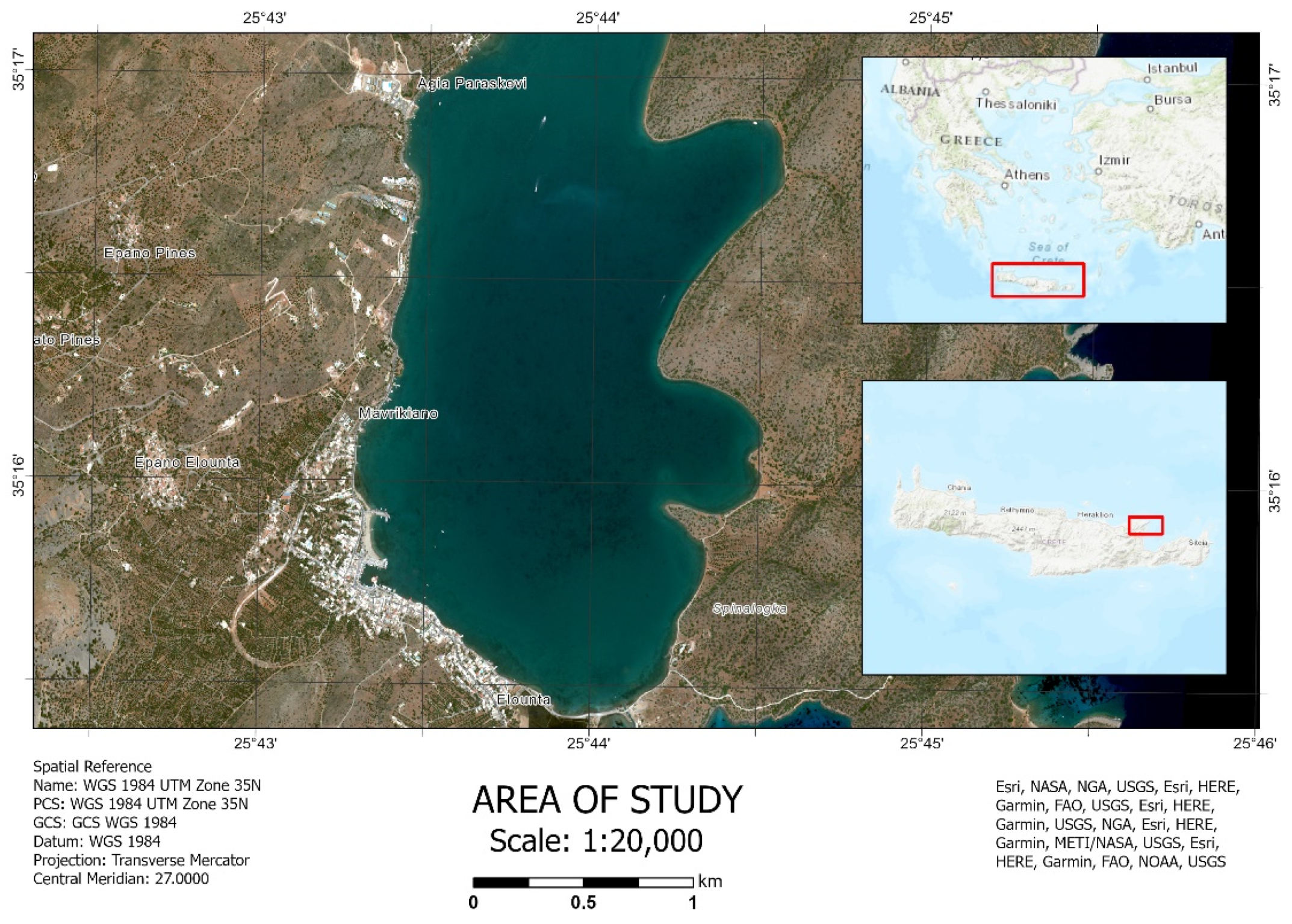
2.1. Study Area
2.2. In Situ Depth Data
2.3. Optical Satellite Images
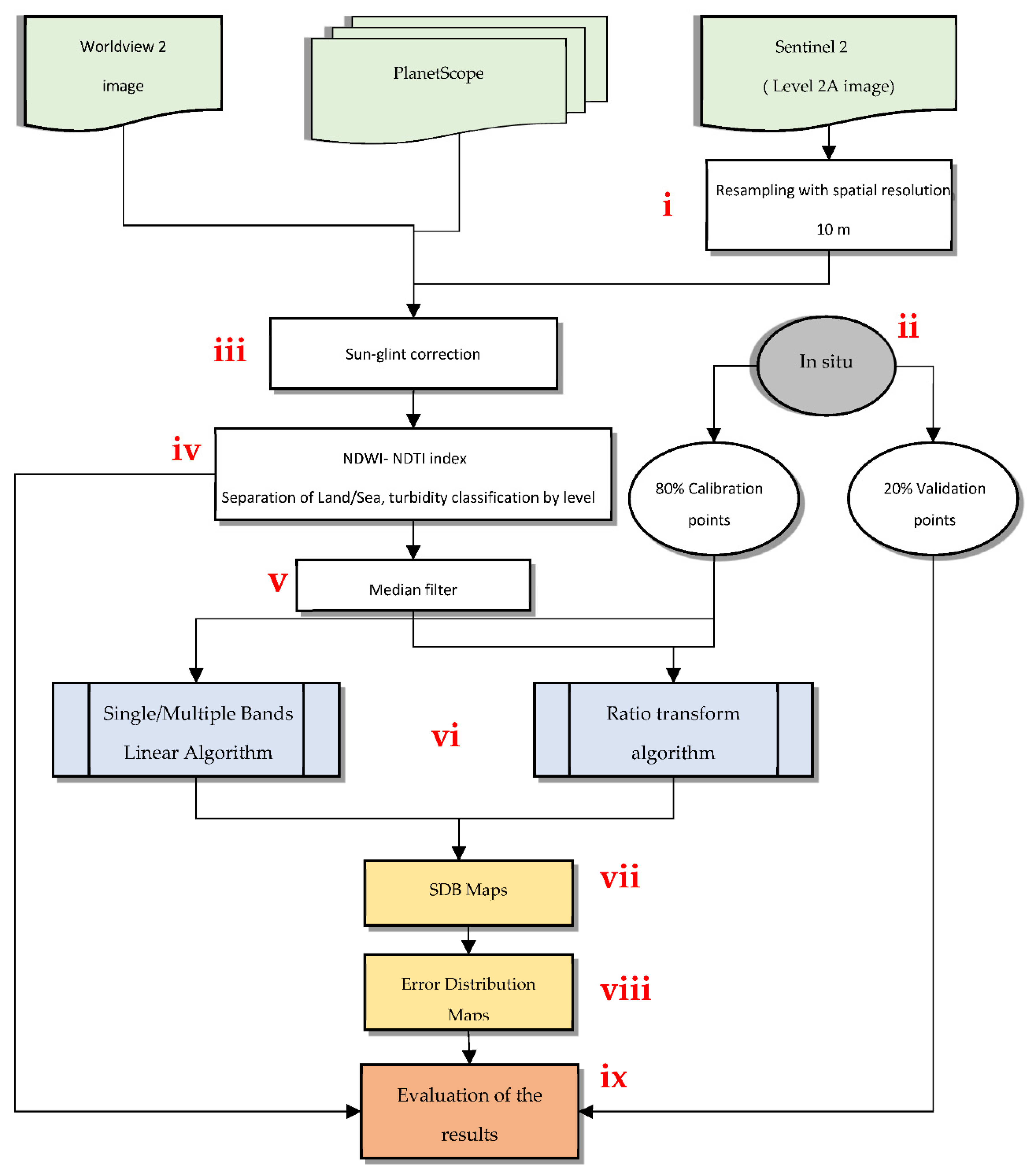
3. Methodology
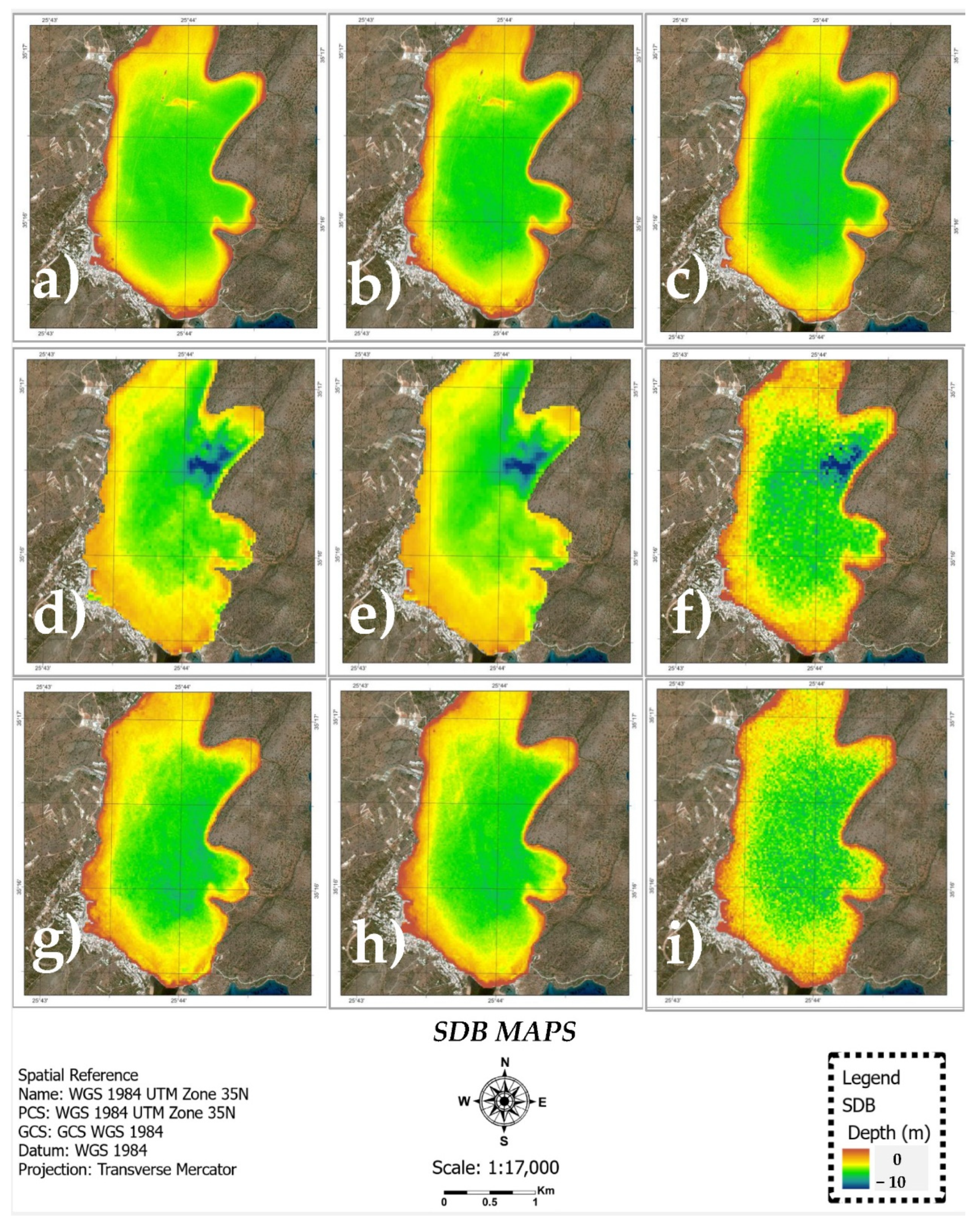
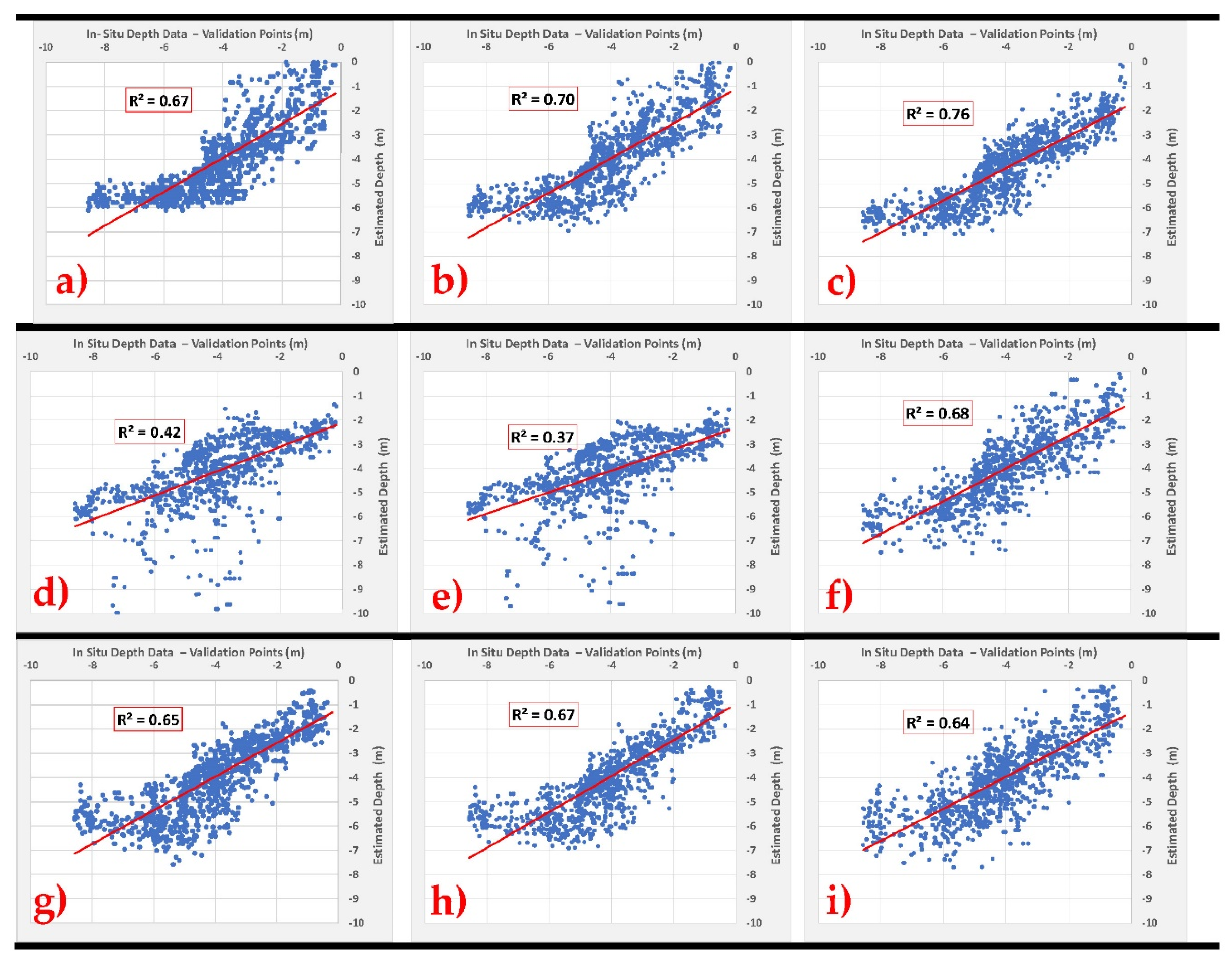
4. Results
5. Discussion
6. Conclusions
Author Contributions
Funding
Institutional Review Board Statement
Informed Consent Statement
Data Availability Statement
Acknowledgments
Conflicts of Interest
References
- Klemas, V.V. The Role of Remote Sensing in Predicting and Determining Coastal Storm Impacts. J. Coast. Res. 2009, 256, 1264–1275. [Google Scholar] [CrossRef] [Green Version]
- Benveniste, J.; Cazenave, A.; Vignudelli, S.; Fenoglio-Marc, L.; Shah, R.; Almar, R.; Andersen, O.; Birol, F.; Bonnefond, P.; Bouffard, J.; et al. Requirements for a Coastal Hazards Observing System. Front. Mar. Sci. 2019, 6, 348. [Google Scholar] [CrossRef] [Green Version]
- Melet, A.; Teatini, P.; Le Cozannet, G.; Jamet, C.; Conversi, A.; Benveniste, J.; Almar, R. Earth Observations for Monitoring Marine Coastal Hazards and Their Drivers. Surv. Geophys. 2020, 41, 1489–1534. [Google Scholar] [CrossRef]
- Janowski, L.; Wroblewski, R.; Dworniczak, J.; Kolakowski, M.; Rogowska, K.; Wojcik, M.; Gajewski, J. Offshore benthic habitat mapping based on object-based image analysis and geomorphometric approach. A case study from the Slupsk Bank, Southern Baltic Sea. Sci. Total Environ. 2021, 801, 149712. [Google Scholar] [CrossRef] [PubMed]
- Summers, G.; Lim, A.; Wheeler, A. A Scalable, Supervised Classification of Seabed Sediment Waves Using an Object-Based Image Analysis Approach. Remote Sens. 2021, 13, 2317. [Google Scholar] [CrossRef]
- Madricardo, F.; Bassani, M.; D’Acunto, G.; Calandriello, A.; Foglini, F. New evidence of a Roman road in the Venice Lagoon (Italy) based on high resolution seafloor reconstruction. Sci. Rep. 2021, 11, 13985. [Google Scholar] [CrossRef]
- Mason, D.C.; Gurney, C.; Kennett, M. Beach topography mapping—A comparsion of techniques. J. Coast. Conserv. 2000, 6, 113–124. [Google Scholar] [CrossRef]
- Porskamp, P.; Rattray, A.; Young, M.; Ierodiaconou, D. Multiscale and Hierarchical Classification for Benthic Habitat Mapping. Geoscience 2018, 8, 119. [Google Scholar] [CrossRef] [Green Version]
- Janowski, L.; Trzcinska, K.; Tegowski, J.; Kruss, A.; Rucinska-Zjadacz, M.; Pocwiardowski, P. Nearshore Benthic Habitat Mapping Based on Multi-Frequency, Multibeam Echosounder Data Using a Combined Object-Based Approach: A Case Study from the Rowy Site in the Southern Baltic Sea. Remote Sens. 2018, 10, 1983. [Google Scholar] [CrossRef] [Green Version]
- Choi, C.; Kim, D.-J. Optimum Baseline of a Single-Pass In-SAR System to Generate the Best DEM in Tidal Flats. IEEE J. Sel. Top. Appl. Earth Obs. Remote Sens. 2018, 11, 919–929. [Google Scholar] [CrossRef]
- Jawak, S.D.; Vadlamani, S.S.; Luis, A.J. A Synoptic Review on Deriving Bathymetry Information Using Remote Sensing Technologies: Models, Methods and Comparisons. Adv. Remote Sens. 2015, 4, 147–162. [Google Scholar] [CrossRef] [Green Version]
- Randazzo, G.; Barreca, G.; Cascio, M.; Crupi, A.; Fontana, M.; Gregorio, F.; Lanza, S.; Muzirafuti, A. Analysis of Very High Spatial Resolution Images for Automatic Shoreline Extraction and Satellite-Derived Bathymetry Mapping. Geoscience 2020, 10, 172. [Google Scholar] [CrossRef]
- Cerra, D.; Gege, P.; Evagorou, E.; Agapiou, A.; Reyes, R.D.L. Monitoring Marine Areas from the International Space Station: The Case of the Submerged Harbor of Amathus. Curr. Trends Web Eng. 2021, 12642, 127–137. [Google Scholar] [CrossRef]
- Chénier, R.; Ahola, R.; Sagram, M.; Faucher, M.-A.; Shelat, Y. Consideration of Level of Confidence within Multi-Approach Satellite-Derived Bathymetry. ISPRS Int. J. Geo-Inform. 2019, 8, 48. [Google Scholar] [CrossRef] [Green Version]
- Pike, S.; Traganos, D.; Poursanidis, D.; Williams, J.; Medcalf, K.; Reinartz, P.; Chrysoulakis, N. Leveraging Commercial High-Resolution Multispectral Satellite and Multibeam Sonar Data to Estimate Bathymetry: The Case Study of the Caribbean Sea. Remote Sens. 2019, 11, 1830. [Google Scholar] [CrossRef] [Green Version]
- Jupp, D. Background and Extensions to Depth of Penetration (DOP) Mapping in Shallow Coastal Waters. 1988. Available online: http://hdl.handle.net/102.100.100/265466?index=1 (accessed on 18 January 2022).
- Lyzenga, D.R. Passive remote sensing techniques for mapping water depth and bottom features. Appl. Opt. 1978, 17, 379–383. [Google Scholar] [CrossRef]
- Lyzenga, D. Remote sensing of bottom reflectance and water attenuation parameters in shallow water using aircraft and Landsat data Remote sensing of bottom reflectance and water attenuation parameters in shallow water using air. Int. J. Remote Sens. 1980, 2, 71–82. [Google Scholar] [CrossRef]
- Lyzenga, D.; Malinas, N.; Tanis, F. Multispectral bathymetry using a simple physically based algorithm. IEEE Trans. Geosci. Remote Sens. 2006, 44, 2251–2259. [Google Scholar] [CrossRef]
- Conger, C.; Hochberg, E.; Fletcher, C.; Atkinson, M. Decorrelating remote sensing color bands from bathymetry in optically shallow waters. IEEE Trans. Geosci. Remote Sens. 2006, 44, 1655–1660. [Google Scholar] [CrossRef]
- Maritorena, S.; Morel, A.; Gentili, B. Diffuse reflectance of oceanic shallow waters: Influence of water depth and bottom albedo. Limnol. Oceanogr. 1994, 39, 1689–1703. [Google Scholar] [CrossRef]
- Adler-Golden, S.; Acharya, P.; Berk, A.; Matthew, M.; Gorodetzky, D. Remote bathymetry of the littoral zone from AVIRIS, LASH, and QuickBird imagery. IEEE Trans. Geosci. Remote Sens. 2005, 43, 337–347. [Google Scholar] [CrossRef]
- Lee, Z.; Carder, K.L.; Mobley, C.D.; Steward, R.G.; Patch, J.S. Hyperspectral remote sensing for shallow waters I A semianalytical model. Appl. Opt. 1998, 37, 6329–6338. [Google Scholar] [CrossRef] [PubMed]
- Stumpf, R.P.; Holderied, K.; Sinclair, M. Determination of water depth with high-resolution satellite imagery over variable bottom types. Limnol. Oceanogr. 2003, 48, 547–556. [Google Scholar] [CrossRef]
- Collings, S.; Botha, E.J.; Anstee, J.; Campbell, N. Depth from Satellite Images: Depth Retrieval Using a Stereo and Radiative Transfer-Based Hybrid Method. Remote Sens. 2018, 10, 1247. [Google Scholar] [CrossRef] [Green Version]
- Cao, B.; Fang, Y.; Jiang, Z.; Gao, L.; Hu, H. Shallow water bathymetry from WorldView-2 stereo imagery using two-media photogrammetry. Eur. J. Remote Sens. 2019, 52, 506–521. [Google Scholar] [CrossRef] [Green Version]
- Sagawa, T.; Yamashita, Y.; Okumura, T.; Yamanokuchi, T. Satellite Derived Bathymetry Using Machine Learning and Multi-Temporal Satellite Images. Remote Sens. 2019, 11, 1155. [Google Scholar] [CrossRef] [Green Version]
- Dickens, K.; Armstrong, A. Application of Machine Learning in Satellite Derived Bathymetry and Coastline Detection. SMU Data Sci. Rev. 2019, 2, 4. [Google Scholar]
- Tonion, F.; Pirotti, F.; Faina, G.; Paltrinieri, D. A Machine Learning Approach to Multispectral Satellite Derived Bathymetry. ISPRS Ann. Photogramm. Remote Sens. Spat. Inf. Sci. 2020, V-3-2020, 565–570. [Google Scholar] [CrossRef]
- Gao, J. Bathymetric mapping by means of remote sensing: Methods, accuracy and limitations. Prog. Phys. Geogr. Earth Environ. 2009, 33, 103–116. [Google Scholar] [CrossRef]
- Manessa, M.D.M.; Haidar, M.; Hartuti, M.; Kresnawati, D.K. Determination of the Best Methodology for Bathymetry Mapping Using Spot 6 Imagery: A Study of 12 Empirical Algorithms. Int. J. Remote Sens. Earth Sci. 2018, 14, 127–136. [Google Scholar] [CrossRef] [Green Version]
- Ashphaq, M.; Srivastava, P.K.; Mitra, D. Review of near-shore satellite derived bathymetry: Classification and account of five decades of coastal bathymetry research. J. Ocean Eng. Sci. 2021, 6, 340–359. [Google Scholar] [CrossRef]
- Warren, M.; Simis, S.; Martinez-Vicente, V.; Poser, K.; Bresciani, M.; Alikas, K.; Spyrakos, E.; Giardino, C.; Ansper, A. Assessment of atmospheric correction algorithms for the Sentinel-2A MultiSpectral Imager over coastal and inland waters. Remote Sens. Environ. 2019, 225, 267–289. [Google Scholar] [CrossRef]
- Ilori, C.O.; Knudby, A. An Approach to Minimize Atmospheric Correction Error and Improve Physics-Based Satellite-Derived Bathymetry in a Coastal Environment. Remote Sens. 2020, 12, 2752. [Google Scholar] [CrossRef]
- Kay, S.; Hedley, J.D.; Lavender, S. Sun Glint Correction of High and Low Spatial Resolution Images of Aquatic Scenes: A Review of Methods for Visible and Near-Infrared Wavelengths. Remote Sens. 2009, 1, 697–730. [Google Scholar] [CrossRef] [Green Version]
- Hedley, J.D.; Harborne, A.; Mumby, P. Technical note: Simple and robust removal of sun glint for mapping shallow-water benthos. Int. J. Remote Sens. 2005, 26, 2107–2112. [Google Scholar] [CrossRef]
- Casal, G.; Monteys, X.; Hedley, J.; Harris, P.; Cahalane, C.; McCarthy, T. Assessment of empirical algorithms for bathymetry extraction using Sentinel-2 data. Int. J. Remote Sens. 2019, 40, 2855–2879. [Google Scholar] [CrossRef]
- Cahalane, C.; Magee, A.; Monteys, X.; Casal, G.; Hanafin, J.; Harris, P. A comparison of Landsat 8, RapidEye and Pleiades products for improving empirical predictions of satellite-derived bathymetry. Remote Sens. Environ. 2019, 233, 111414. [Google Scholar] [CrossRef] [PubMed]
- Goodman, J.A.; Lee, Z.; Ustin, S. Influence of atmospheric and sea-surface corrections on retrieval of bottom depth and reflectance using a semi-analytical model: A case study in Kaneohe Bay, Hawaii. Appl. Opt. 2008, 47, F1–F11. [Google Scholar] [CrossRef] [PubMed] [Green Version]
- Bramante, J.F.; Raju, D.K.; Sin, T.M. Multispectral derivation of bathymetry in Singapore’s shallow, turbid waters. Int. J. Remote Sens. 2012, 34, 2070–2088. [Google Scholar] [CrossRef]
- Lacaux, J.; Tourre, Y.; Vignolles, C.; Ndione, J.; Lafaye, M. Classification of ponds from high-spatial resolution remote sensing: Application to Rift Valley Fever epidemics in Senegal. Remote Sens. Environ. 2007, 106, 66–74. [Google Scholar] [CrossRef]
- Kopp, M.; Purgathofer, W. Efficient 3 × 3 Median Filter Computations, Technical Report TR-186-2-94-18; Institute of Computer Graphics and Algorithms, Visualization and Animation Group, Vienna University of Technology: Vienna, Austria, 1994. [Google Scholar]
- Lyzenga, D.R. Shallow-water bathymetry using combined lidar and passive multispectral scanner data. Int. J. Remote Sens. 1985, 6, 115–125. [Google Scholar] [CrossRef]
- Vahtmäe, E.; Kutser, T. Airborne mapping of shallow water bathymetry in the optically complex waters of the Baltic Sea. J. Appl. Remote Sens. 2016, 10, 025012. [Google Scholar] [CrossRef]
- Martens, H.A.; Dardenne, P. Validation and verification of regression in small data sets. Chemom. Intell. Lab. Syst. 1998, 44, 99–121. [Google Scholar] [CrossRef]
- Casal, G.; Hedley, J.D.; Monteys, X.; Harris, P.; Cahalane, C.; McCarthy, T. Satellite-derived bathymetry in optically complex waters using a model inversion approach and Sentinel-2 data. Estuarine Coast. Shelf Sci. 2020, 241, 106814. [Google Scholar] [CrossRef]
- Gabr, B.; Ahmed, M.; Marmoush, Y. PlanetScope and Landsat 8 Imageries for Bathymetry Mapping. J. Mar. Sci. Eng. 2020, 8, 143. [Google Scholar] [CrossRef] [Green Version]
- Minghelli-Roman, A.; Goreac, A.; Mathieu, S.; Spigai, M.; Gouton, P. Comparison of bathymetric estimation using different satellite images in coastal sea waters. Int. J. Remote Sens. 2009, 30, 5737–5750. [Google Scholar] [CrossRef]


| A/A | Satellite | Product Name | Resolution | Date Acquisition | Sensing Time | Sun Zenith Angle—º | Sun Azimuth Angle—º | Cloud Coverage % |
|---|---|---|---|---|---|---|---|---|
| 1 | Worldview 2 | 19MAY25091947-M2AS-012814699010_01_P001 | 2 m | 19/05/2019 | 09:19 | 18.50 | 136.40 | 0 |
| 2 | PlanetScope | 20190518_074518_1048_3B_udm2 | 3 m | 18/05/2019 | 07:45 | 53.88 | 105.85 | 1.35 |
| 3 | Sentinel 2 | S2A_MSIL2A_20190513T085601_N0212_R007_T35SLV_20190513T112941 | 10 m | 13/05/2019 | 08:56 | 22.36 | 136.42 | 1.66 |
| Worldview 2 | Sentinel 2 | PlanetScope | |||||||||||||||
|---|---|---|---|---|---|---|---|---|---|---|---|---|---|---|---|---|---|
| SBLA | MBLA | RTA | SBLA | MBLA | RTA | SBLA | MBLA | RTA | |||||||||
| Bands | R2 (%) | Bands | R2 (%) | Bands | R2 (%) | Bands | R2 (%) | Bands | R2 (%) | Bands | R2 (%) | Bands | R2 (%) | Bands | R2 (%) | Bands | R2 (%) |
| B1 | 0.13 | B 1,2 | 0.27 | B 1,2 | 0.38 | B1 | 0.30 | B 1,2 | 0.31 | B 1,2 | 0.00 | B1 | 0.57 | B 1,2 | 0.63 | B 1,2 | 0.62 |
| B2 | 0.32 | B 1,3 | 0.60 | B 1,3 | 0.69 | B2 | 0.30 | B 1,3 | 0.40 | B 1,3 | 0.28 | B2 | 0.68 | B 1,3 | 0.67 | B 1,3 | 0.60 |
| B3 | 0.65 | B 1,4 | 0.64 | B 1,4 | 0.67 | B3 | 0.45 | B 1,4 | 0.05 | B 2,3 | 0.66 | B3 | 0.65 | B 1,2,3 | 0.67 | B 2,3 | 0.43 |
| B4 | 0.65 | B 1,2,3 | 0.54 | B 2,3 | 0.74 | B 1,2,3 | 0.37 | B4 | 0.49 | B 2,3 | 0.69 | ||||||
| B 1,2,4 | 0.61 | B 2,4 | 0.61 | B 1,2,4 | 0.08 | ||||||||||||
| B 1,3,4 | 0.67 | B 3,4 | 0.12 | B 1,3,4 | 0.10 | ||||||||||||
| B 1,2,3,4 | 0.64 | B 1,2,3,4 | 0.13 | ||||||||||||||
| B 2,3 | 0.57 | B 2,3 | 0.39 | ||||||||||||||
| B 2,4 | 0.64 | B 2,4 | 0.05 | ||||||||||||||
| B 2,3,4 | 0.66 | B 2,3,4 | 0.10 | ||||||||||||||
| B 3,4 | 0.69 | B 3,4 | 0.07 | ||||||||||||||
| no | Algorithm | Satellite | SDB Points | Equations | Validation Points | RMSE (m) | R2 |
|---|---|---|---|---|---|---|---|
| 1 | SBLA | WV2 | 4521 | y = 41.865x − 92.059 | 1145 | 1.08 | 0.67 |
| 2 | S2A | y = 12.095x − 38.316 | 1.46 | 0.42 | |||
| 3 | PlanetScope | y = 33.417x − 97.458 | 1.11 | 0.65 | |||
| 4 | MBLA | WV2 | y = 23.033x − 107.45 | 1.03 | 0.70 | ||
| 5 | S2A | y = 6.4394x − 40.255 | 1.52 | 0.37 | |||
| 6 | PlanetScope | y = 14.885x − 83.271 | 1.08 | 0.67 | |||
| 7 | Ratio Transform algorithm | WV2 | y = −149.97x + 142.89 | 1.01 | 0.76 | ||
| 8 | S2A | y = −145x + 140.8 | 1.06 | 0.68 | |||
| 9 | PlanetScope | y = −280.12x + 276.64 | 1.13 | 0.64 |
Publisher’s Note: MDPI stays neutral with regard to jurisdictional claims in published maps and institutional affiliations. |
© 2022 by the authors. Licensee MDPI, Basel, Switzerland. This article is an open access article distributed under the terms and conditions of the Creative Commons Attribution (CC BY) license (https://creativecommons.org/licenses/by/4.0/).
Share and Cite
Evagorou, E.; Argyriou, A.; Papadopoulos, N.; Mettas, C.; Alexandrakis, G.; Hadjimitsis, D. Evaluation of Satellite-Derived Bathymetry from High and Medium-Resolution Sensors Using Empirical Methods. Remote Sens. 2022, 14, 772. https://doi.org/10.3390/rs14030772
Evagorou E, Argyriou A, Papadopoulos N, Mettas C, Alexandrakis G, Hadjimitsis D. Evaluation of Satellite-Derived Bathymetry from High and Medium-Resolution Sensors Using Empirical Methods. Remote Sensing. 2022; 14(3):772. https://doi.org/10.3390/rs14030772
Chicago/Turabian StyleEvagorou, Evagoras, Athanasios Argyriou, Nikos Papadopoulos, Christodoulos Mettas, George Alexandrakis, and Diofantos Hadjimitsis. 2022. "Evaluation of Satellite-Derived Bathymetry from High and Medium-Resolution Sensors Using Empirical Methods" Remote Sensing 14, no. 3: 772. https://doi.org/10.3390/rs14030772