Article

Integration of DInSAR Time Series and GNSS Data for Continuous Volcanic Deformation Monitoring and Eruption Early Warning Applications

Department of Geological Sciences, The Collaborative Institute of Research in Environmental Sciences (CIRES), University of Colorado Boulder, Boulder, CO 80309, USA
*
Author to whom correspondence should be addressed.
Remote Sens. 2022, 14(3), 784; https://doi.org/10.3390/rs14030784
Submission received: 1 January 2022 / Revised: 25 January 2022 / Accepted: 26 January 2022 / Published: 8 February 2022

Abstract

:
With approximately 800 million people globally living within 100 km of a volcano, it is essential that we build a reliable observation system capable of delivering early warnings to potentially impacted nearby populations. Global Navigation Satellite System (GNSS) and satellite Synthetic Aperture Radar (SAR) document comprehensive ground motions or ruptures near, and at, the Earth’s surface and may be used to detect and analyze natural hazard phenomena. These datasets may also be combined to improve the accuracy of deformation results. Here, we prepare a differential interferometric SAR (DInSAR) time series and integrate it with GNSS data to create a fused dataset with enhanced accuracy of 3D ground motions over Hawaii island from November 2015 to April 2021. We present a comparison of the raw datasets against the fused time series and give a detailed account of observed ground deformation leading to the May 2018 and December 2020 volcanic eruptions. Our results provide important new estimates of the spatial and temporal dynamics of the 2018 Kilauea volcanic eruption. The methodology presented here can be easily repeated over any region of interest where an SAR scene overlaps with GNSS data. The results will contribute to diverse geophysical studies, including but not limited to the classification of precursory movements leading to major eruptions and the advancement of early warning systems.

Graphical Abstract

1. Introduction

Volcanic eruptions, earthquakes, and tsunamis occur over numerous spatial and temporal scales. Although these phenomena are often studied individually, there is frequently interconnectivity between disaster types. For example, concentrated swarms of earthquakes, elevated readings of gas emission, and increased ground motion over volcanic regions may indicate an impending eruption [1,2,3,4,5,6,7,8]. Most active volcanoes around the world are monitored using geodetic data sets such as Synthetic Aperture Radar (SAR) and Global Navigation Satellite System (GNSS) data, in conjunction with other ground-based instruments, with the goal of providing early warning for major eruptions and reducing risk to nearby populations or infrastructure [9]. While several studies have attempted to forecast or model potential volcano hazards using remote sensing techniques [2,10,11,12,13,14,15,16], there is currently no single framework in place that simultaneously consolidates geodetic data from multiple sensors, freely provides scientists with near real-time continuous time series products and is capable of distinguishing and broadcasting geophysical events.
The GeoScience CyberInfrastructure Framework (GeoSCIFramework or GSF) project aims to improve intermediate-to-short term forecasts of catastrophic natural hazard events, allowing researchers to instantly detect phenomena and reveal more suppressed, long-term motions of Earth’s surface at unprecedented spatial and temporal resolutions. These goals will be accomplished by applying big data analytics and training machine learning algorithms to recognize patterns across various data signals during noteworthy events. When complete, the system will be capable of processing and delivering large streams of near real-time data from a mix of Differential Interferometric SAR (DInSAR) imagery, GNSS, and other geodetic-related sensors, as well as seismic, gas emission, and thermal data.
DInSAR quantifies line-of-sight (LOS) ground deformation with mm-cm precision, and GNSS data delivers precise point positioning and timing data to determine exact location and deformation measurements, also with mm-cm scale precision. Furthermore, DInSAR processing can be combined with GNSS data to obtain 3D ground surface motions [17,18,19,20]. Together, these time series produce high resolution, sub-centimeter precision measurements of ground deformation over large swaths of Earth’s surface with dense spatiotemporal coverage, which provides scientists with a greater understanding of crustal or shallow subsurface dynamics over volcanic regions.
We focus on generating an automated DInSAR time series processing routine that is integrated with GNSS data into a unified deformation field to provide more constrained deformation rates and vector measurements related to volcanic activity. We process Sentinel-1A/B SAR data into time series over Hawaii from November 2015 to April 2021 and integrate those results with GNSS data at various station positions (Figure 1). The DInSAR + GNSS integrated time series can be used to describe the full extent of ground motions through time with decreased uncertainty in three directions of motion (east-west, north-south, and up-down). We present the unified DInSAR and GNSS time series and compare them to the original datasets.
Our region of interest is over the Big Island of Hawaii. Unlike most volcanic systems, Hawaii experiences frequent eruptive activity and provides an opportunity for scientists to record extensive observations over multiple events. Kilauea volcano has erupted 34 times since 1952 [24]. Two volcanic eruptions are captured within our time series between November 2015 and April 2021. The first eruption occurred in May 2018, when the lava lake within the Halema’uma’u crater (collocated with CRIM station, Figure 1) drained following an intrusion into, and subsequent eruption from, the Puʻu ʻŌʻō crater (collocated with NUPM station, Figure 1) and Kilauea’s lower East Rift Zone (ERZ) (Yellow polygon, Figure 1). Sudden changes in lava lake levels, increased micro-seismicity around Kilauea’s summit, and deformation along the NE strike of the ERZ were all precursory indications reported by the Hawaiian Volcano Observatory (HVO) that an impending eruption might occur [10,25]. According to [26], an obstruction in the magma plumbing system at Puʻu ʻŌʻō volcano caused widespread pressurization in the volcano, driving magma into the lower, eastern flank. Activity over the ERZ decelerated by September 2018 and remained quiet until December 2020, when a summit eruption that continued through May 2021 refilled the lava lake within the Halema‘uma‘u crater [24]. Although we observe this activity within the separate datasets, DInSAR and GNSS, as shown in Section 2, by integrating the two geodetic datasets together, we recover a 3-D spatial map, instead of 1-D LOS motion, with the resolution of the DInSAR images, that includes time series for motion in the east-west, north-south, and up direction, at each location. In addition, there is a significant improvement in the accuracy of each component of motion (east, north, up) relative to either the DInSAR or GNSS data alone, as presented in Section 3 and Section 4.

2. Materials and Methods
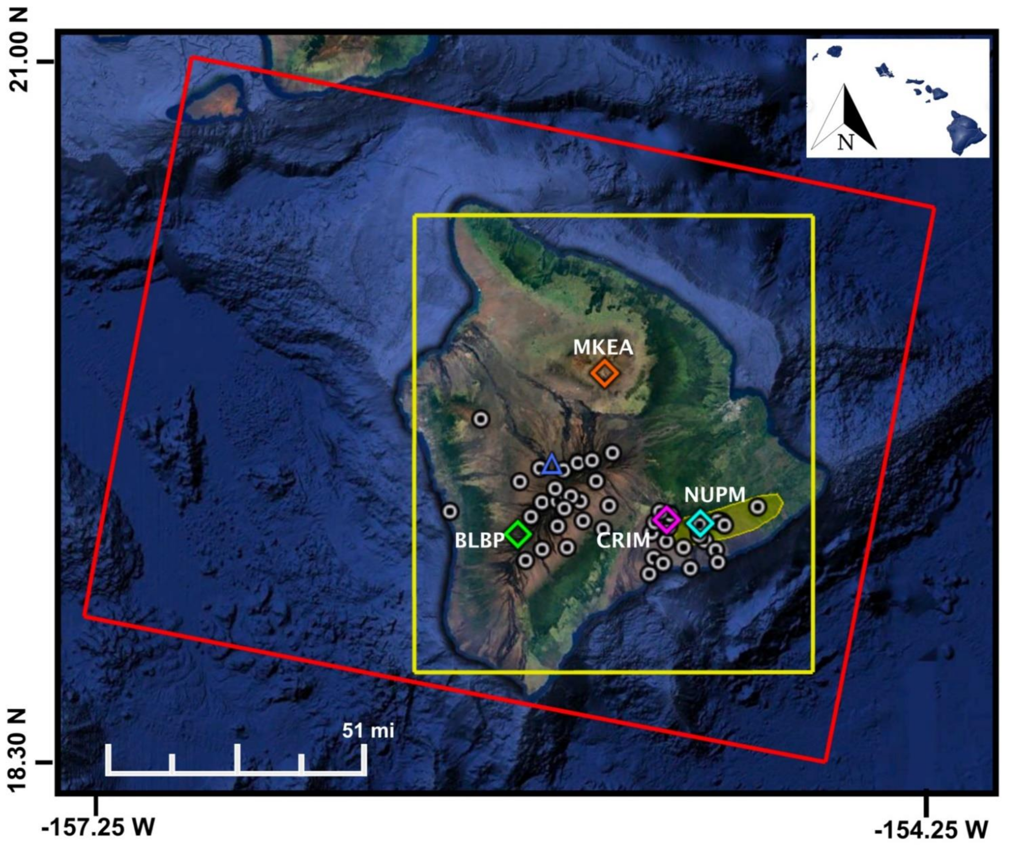
The automated DInSAR processing routine was separated into three different components. The first section (Stage 1) was built based on GMTSAR source code [27,28] to process single look complex (SLC) DInSAR satellite imagery into interferograms using the small baseline subset (SBAS) method [29] performed in parallel. The second phase (Stage 2) applies the New SBAS (NSBAS) inversion [30] method to the GMTSAR interferograms of Stage 1 and generates the DInSAR time series and the cumulative deformation map. Finally, the third component (Stage 3) produces integrated 3D displacements using the LOS deformation from Stage 2, the geometry of the SAR acquisition, and precise, 3D vector positioning measurements [12,18,19,20]. The routine can process the fused data at a single pixel, which is delivered as a plotted time series, or as an interpolated displacement map over a larger region, created from an array of available GNSS stations within the extent of the SAR scene.

2.1. Data

For this study, 250 descending Sentinel-1A/B SLC images were acquired between November 2015 to April 2021 along Path 87 Scene 526 (Figure 1; Supplementary Material List S1) through the Alaskan Satellite Facility (ASF) Vertex portal [21]. Twenty-four-hour final solution GNSS data was managed by the USGS HVO and archived by the UNAVCO GAGE facility; processed time series were generated by and distributed through NGL [22,23]. Data from 48 GNSS stations over Hawaii (Table 1, Figure 1) were obtained over the same period of time, decimated to match the sampling rate of the InSAR time series, and used to create the interpolated map for this study. We used the ordinary kriging interpolation algorithm [31,32,33] supported by an exponential distribution model to construct standard variograms from the 48 GNSS station data.
While GNSS is known for its high precision in the horizontal directions (east and north), estimates of vertical motion have a larger uncertainty [34,35]. On the other hand, with an incidence angle range of 18.3° to 46.8°, DInSAR sensors are most sensitive to vertical displacements and can help to improve ground velocity estimates in the up direction [20,35]. Our integrated results provide a better representation, and therefore, a better understanding of the volcanic deformation pattern and subsurface-surface behavior through time. The workflow presented here can be easily repeated or applied to other locations where GNSS data falls within an SAR scene footprint.

2.2. Building Interferograms

DInSAR processing is challenging and complex in that several improvements, including orbital, topographic, and atmospheric corrections, must be applied to isolate the deformation signal. As we consider an automated system that will be streaming continuous Sentinel-1A/B data over Hawaii Island, we must decide how these corrections are applied and systematized within the processing routine. This first component requires several input parameters and files to run, including the SAR images, the corresponding orbital correction files, a Digital Elevation Model (DEM), and the number of allowed days between potential interferometric image pairs.
For the time series presented in this paper, we used only precise orbital corrections on each Sentinel-1 A/B SLC image. These precise files, which were also obtained through the ASF Vertex portal [21], are not available to users until two weeks after the SAR image is acquired by the Sentinel satellite. Thus, for the real-time automated system, and due to the Sentinel-1A/B satellites’ repeat period of 6–12 days, the most recent SAR image acquisitions over the region of interest were first processed using real-time orbital corrections and then updated with the precise corrections two weeks later. We thoroughly review the effects of real-time vs. precise orbital corrections in [9] and determine that the use of real-time orbits is sufficient for early-warning applications. For the topographic correction, we used a 30 m resolution SRTM DEM that completely covers the SAR image footprint.
After the orbital and topographic corrections are applied, the complex interferogram is formed. We allowed the algorithm to pair any two images that were obtained within 35 days of each other. From the 250 descending SLC images acquired between November 2015 and April 2021, 671 interferometric image pairs were successfully generated (Supplementary Material List S2). For each pair, interferometric products of phase, coherence, phase gradient, and LOS displacement were constructed in both radar and geographical coordinates (Figure 2). The code utilizes the Snaphu phase unwrapping method [36] and geocodes all interferometric output products. These outputs are formatted as GMT-compatible grids, which easily convert to GeoTIFF or other GDAL-compatible raster drivers.

2.3. DInSAR Time Series Generation

The second component of the automated system uses the GIAnT software [37] to construct LOS displacement maps and time series. In GIAnT, unwrapped interferograms are converted to units of millimeters before any processing takes place. The software assembles the input data, the unwrapped interferograms, coherence maps, masks, and metadata, into binary files and a composite HDF5 file that is compatible with GIAnT processing.
The user can choose between several atmospheric model corrections, including the European Centre for Medium-Range Weather Forecasts (ECMWF) model, which is built into the software so that the atmospheric files are pulled and applied automatedly. Currently, ECMWF is in the midst of migrating its data to an updated server, rendering the files temporarily unavailable. Therefore, for this study, the Generic Atmospheric Correction Online Service (GACOS) atmospheric model correction was applied. The GACOS model integrates the ECMWF atmospheric files with continuous GNSS tropospheric delay estimates, which currently must be manually ordered through the online portal [38,39,40,41]. The goal is to incorporate it into automated processing in the future.
The user can also choose between different time series inversion methods, available from GIAnT, to estimate filtered time series. The SBAS and NSBAS techniques, which are implemented here, are applicable when the differential interferograms have a small spatial baseline, a characteristic of Sentinel-1A/B data [29,30]. In particular, the NSBAS technique also estimates DEM errors and compensates for pixels that have missing observations. This inversion method estimates the LOS phase change of each pixel independently using a linear system.
For Stage 1, the automated scripts ran using high-performance computing nodes on the SUMMIT supercomputer located at the University of Colorado, Boulder, for approximately eight hours to produce 694 interferograms between November 2015 and April 2021. The NSBAS technique applies inversion on the 694 input interferograms to generate a time series with a cumulative displacement measurement for every date, or time-slice, included within the data. In this case, the time series produced 275 time-slices (See Figure 3). The atmospheric correction and inversion process in Stage 2 took approximately two hours to complete. Once the historical data has been processed, however, adding a new acquisition to the time series takes on the order of a couple of hours to fully acquire and process the necessary data, then output all the updated DInSAR-related products and time series.

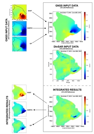
2.4. Integration of Geodetic Datasets

We integrate our DInSAR time series with GNSS data from 48 stations over Hawaii to produce 3D high-resolution cumulative displacement maps with corresponding errors. The 24 h final GNSS solutions are provided in three components (east, north, up) and aligned to the local, fixed Pacific plate reference frame to minimize linear trends of the tectonic plate motion. It is worth noting that NGL also provides solutions aligned to the International GNSS Service-14 (IGS14) reference frame, which is based on the International Terrestrial Reference Frame (ITRF) and holds a no-net-rotation (NNR) [42]. We present a comparison of the results from both reference frames in the Supplementary Material (Figures S1–S3).
First, we temporally subset the GNSS data from 48 stations to extract the data corresponding to the interval of the DInSAR time series. For each time step, we used the ordinary kriging algorithm and the 3D displacements from the 48 stations to compute a variogram. The spatial covariance of the GNSS data determines the structure of the variogram, and the weights were calculated from the data using an exponential distribution model to interpolate undefined points across the spatial field [31,32]. The kriging algorithm outputs three cumulative displacement maps (east, north, and up) with the same discretization and geocoding as the DInSAR output from Section 2.2 (Figure 4), [12,18,19,43,44,45].
To combine all the geodetic displacement data into a single time series product, we expand on the DInSAR+GNSS velocity integration method developed by [12]. The method uses a Bayesian statistical modeling approach in conjunction with Markov random field (MRF) theory to combine datasets with varying spatio-temporal extents. Integration of DInSAR and GNSS high-resolution, 3D surface displacement measurements was achieved by minimization of the energy function related to the corresponding Gibbs random field (GRF) distribution, in which the joint probability density of the variables are positive [12,18,19,33]. The energy function is as follows:
U b / a = i = 1 N ( b i a i ) 2 2 σ i 2
where U b a is the likelihood energy, b is the observation with uncertainty σ , a is the unknown parameter, and N is the number of observations or pixels within the acquisition. The resulting adaptation of Equation (1) to our geodetic displacement datasets is:
U d L O S , d x G P S , d y G P S , d z G P S / d x , d y , d z = i = 1 N C L O S ( d L O S S x L O S d x S y L O S d y S z L O S d z ) 2 + C x G P S ( d x G P S d x ) 2 + C y G P S ( d y G P S d y ) 2 + C z G P S ( d z G P S d z ) 2
with coefficients:
C L O S = 1 2 ( σ L O S ) 2 ,           C x G P S = 1 2 ( σ x G P S ) 2 , C y G P S = 1 2 ( σ y G P S ) 2 , C z G P S = 1 2 ( σ z G P S ) 2
where σ is the standard deviation for the measurements, d L O S   is the cumulative LOS displacement, S x L O S , S y L O S , S z L O S are the unit vectors pointing from the ground to the satellite, and d x G P S , d y G P S , d z G P S are the 3D displacements from the kriging interpolated GNSS data. The remaining equation details are outlined in the Supplementary Material (Equations S1–S8).
Uncertainties associated with the 3D displacement maps and the plotted time series are automatically generated with the corresponding products. These are integrated using the same methodology as the observations and are a combination of the raw GNSS data uncertainties and the LOS DInSAR uncertainties (Equations S6–S8 in Supplementary Material). For the 3D displacement maps, an additional error is introduced when we interpolate data from the 48 GNSS stations into a variogram using the ordinary kriging algorithm. We present the error analysis for that integration in the Supplementary Material (Figures S4 and S5).

3. Results

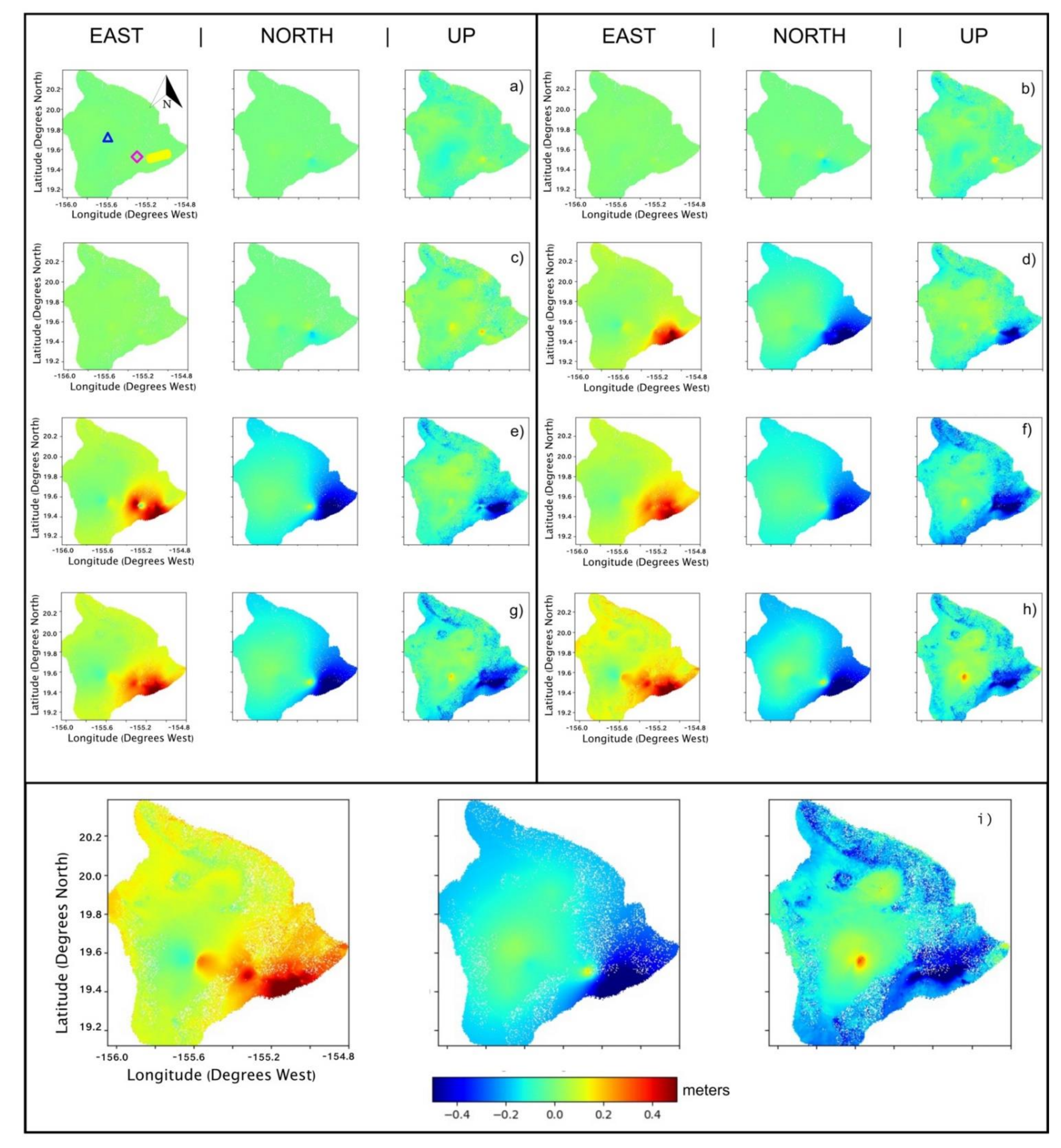
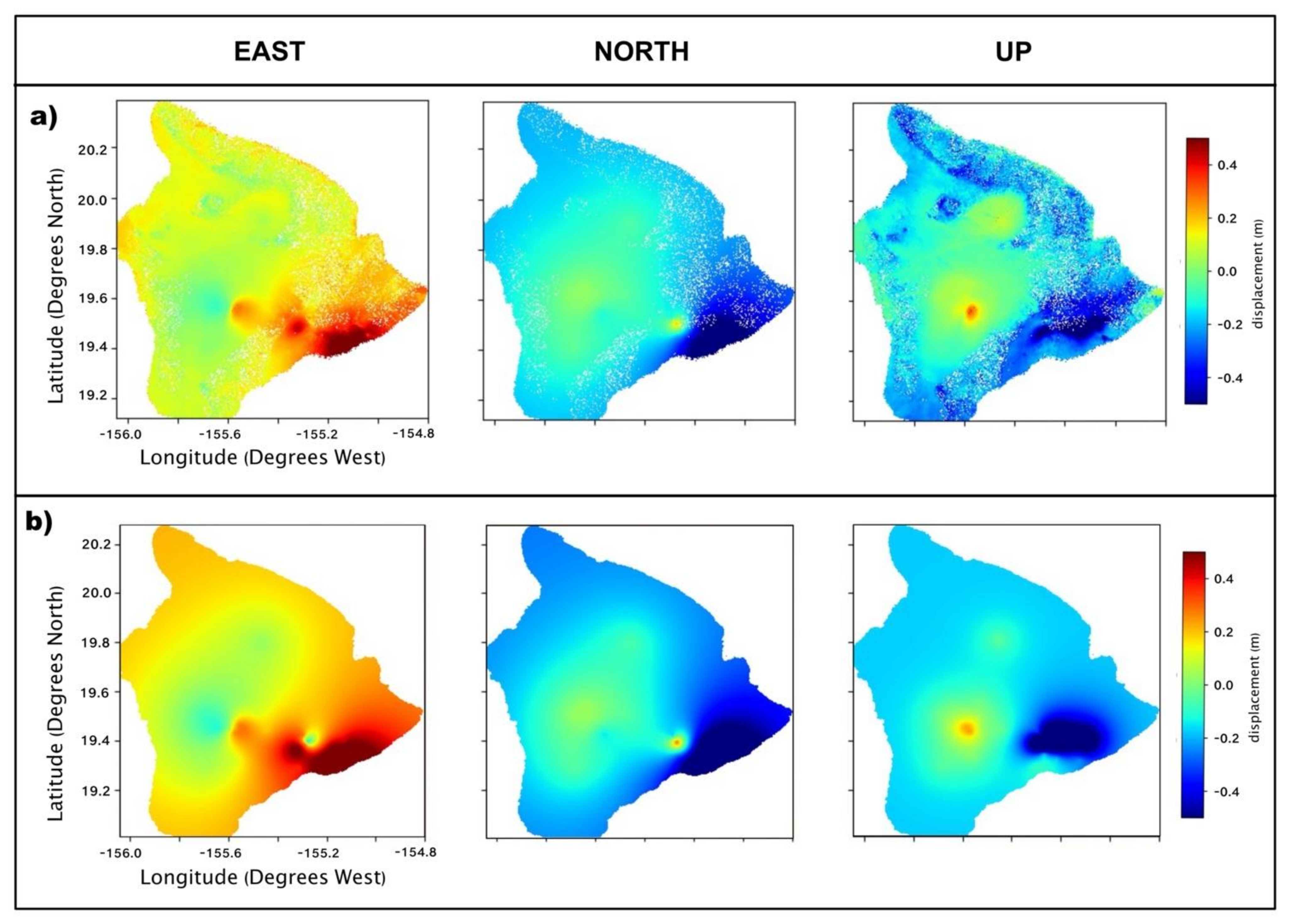
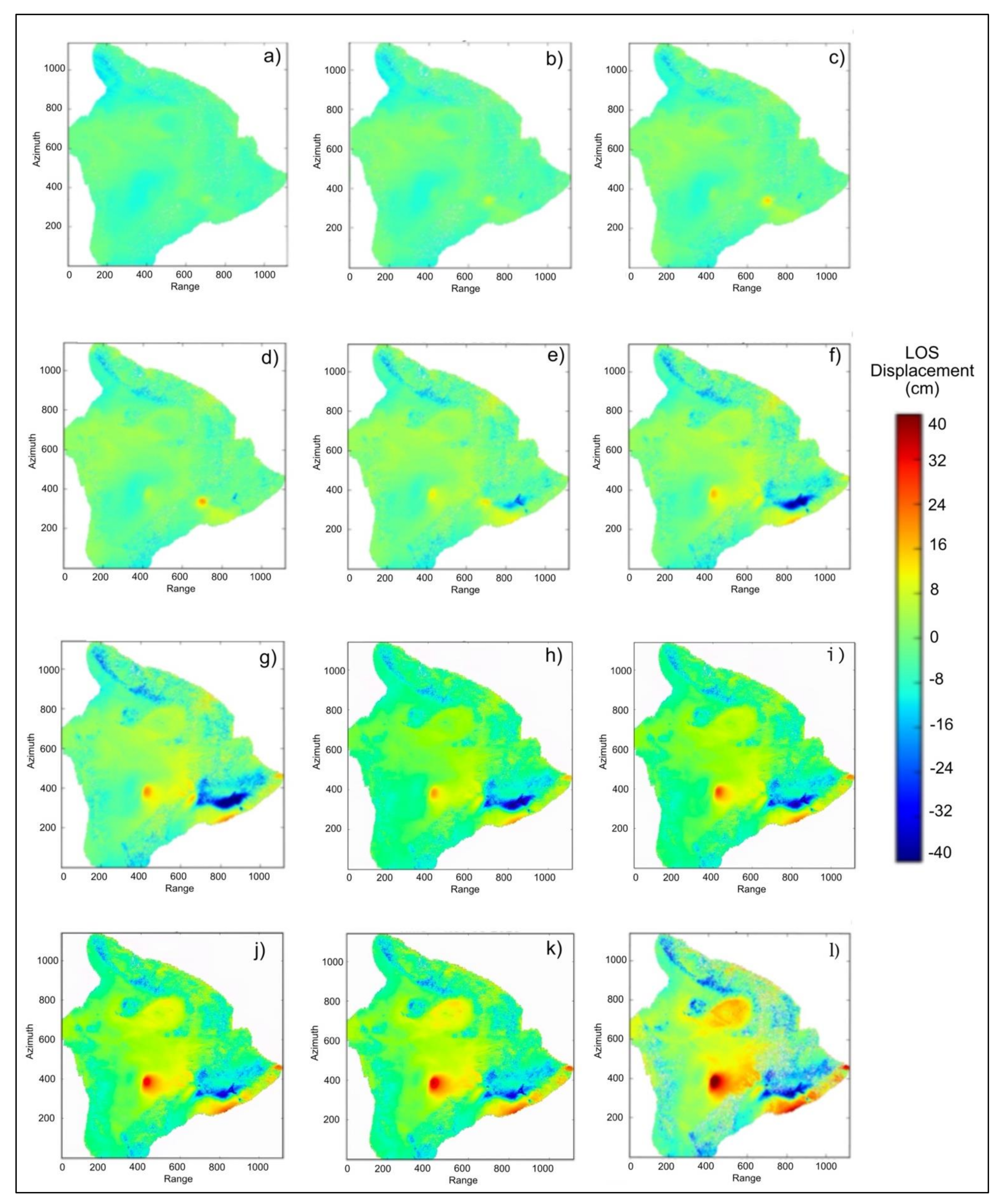
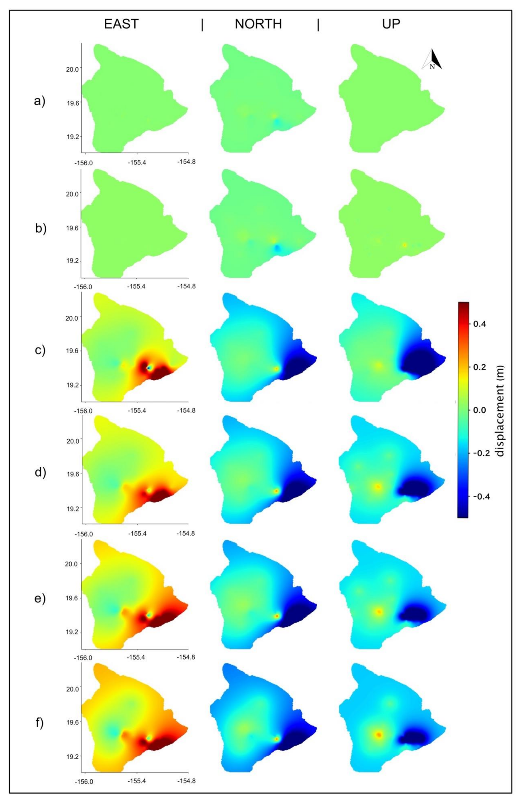
3.1. Cumulative Deformation Maps

The automated processing system can provide the assimilated DInSAR+GNSS time series to users in multiple ways. Over large areas, the code produced 3D high-resolution cumulative displacement maps and the corresponding uncertainties for each individual date or time-step of the series. Figure 5 shows the evolution of 3D surface motions captured in our time series, revealing the long-term deformation response to the May 2018 and December 2020 eruptions. The pixel resolution of the fused products was 100 m, the same as the DInSAR results.
Slight inflation (~10 cm) over the Kilauea volcano (purple diamond, Figure 1 and Figure 5) was observed in the fused DInSAR+GNSS results as early as November 2016, nearly 1.5 years before the eruption took place (Figure 5a). By August 2017 (Figure 5b), cumulative inflation over Kilauea reached +26 cm. This magma intrusion is further supported by the pattern observed over the same region in the north-component subplot, in which the southern flank of Kilauea moved approximately 15 cm further south, and the northern flank moved 8 cm further north.
Upward motion over Mauna Loa volcano (blue triangle, Figure 1 and Figure 5) also began to increase in August 2017. By February 2018 (Figure 5c), this inflation pattern was recognizable over Mauna Loa, where the ground reached +16 cm of uplift and was obvious over the Kilauea volcano after reaching +30 cm of total uplift. Over the following months, inflation at Mauna Loa began to slow, while it continued to increase at a similar/opposite rate over Kilauea. This interaction between the two volcanic systems has been studied before [46,47,48,49] and provides further evidence of upper mantle links and magma transportation.
On 30 April 2018, the Pu’u ‘Ō’ō eruptive vent collapsed [48,49,50], and on May 4, a Mw 6.9 earthquake occurred on the south flank of Kilauea, initiating the 2018 volcanic eruption. Our integrated results from 5 May 2018 (Figure 5d) recorded the 43 cm southeast ground rupture of the earthquake. Next, the sudden evacuation of subsurface material resulted in a rapid −10 cm ground deflation at Kilauea’s crater and −80 cm over the ERZ near Puʻu ʻŌʻō volcano (yellow polygon, Figure 1 and Figure 5a).
As this eruptive activity began over the ERZ, the ground at Mauna Loa inflated in the east-west directions from a continued subsurface magma injection. This divergent, horizontal pattern became more obvious by June 2018 (Figure 5e), after Mauna Loa experienced an additional +3 cm of uplift (a net total of 13 cm). A closer look at deformation over the Kilauea crater in June 2018 indicated additional, sudden ruptures that moved the localized ground 25 cm to the west and in the vertical direction, Kilauea crater subsided another −9 cm. This deformation was likely due to the accelerated down-drop of Kilauea’s caldera combined with 62 summit collapse events between May 16 and August 2 [48,49]. HVO reported that some collapse events released energy equivalent to a Mw 4.7 to 5.4 earthquake; our results captured these details.
Another interesting feature includes the three zones of subsidence radially surrounding Kilauea’s summit and the Halema’uma’u crater. These deflated regions are spatially separated by ~120 degrees. The two zones to the north and the southwest both experienced between −35 and −45 cm subsidence. The southeast leg of the three-pronged sinking feature fed into the ERZ, which has subsided more than −1.17 m to date. No active surface lava was observed after 4 September 2018 [48,49], but the ground surface over the ERZ continued to deflate through December of that year (Figure 5f), reaching a cumulative minimum of −1.32 m.
Soon after, the cumulative subsidence from the ERZ began to shrink, indicating that during the recovery from the 2018 eruption, the subsurface chambers may have begun refilling with magma. In November 2019 (Figure 5g), the east-west inflation pattern over Mauna Loa became more prominent, and uplift reached a total of +21 cm. The north-south component revealed that the Kilauea crater also recovered 17 cm of motion to the north (against the dominant southeastern motion of the ERZ and the coastline just south of the region) and regained +26 cm in vertical surface height.
Over the next year leading to the December 2020 summit eruption, another +11 cm of upward motion occurred at Mauna Loa (net total of +32 cm), and +14 cm occurred along the ERZ (net total of −83 cm) (Figure 5h). Immediately following the summit eruption, the ground height at Kilauea summit measured a total of +20 cm, while the region surrounding the crater subsided once more, decreasing the total ground height by −30 cm. In mid-April 2021, when our time series ended (Figure 5I), a cumulative total of +21 cm of uplift occurred at the Kilauea crater, and +46 cm of uplift had occurred at Mauna Loa in response to the 2018 eruption and 2020 summit eruptions. Kilauea’s surrounding volcanic flank and the ERZ experienced −50 cm and −1.0 m of subsidence, respectively.
These products allowed us to observe the total cumulative deformation pattern in the east, north, and up directions over the entire island from November 2015 to April 2021 with improved accuracy and detail. The 3D cumulative displacement maps provided new information regarding the pre-, during-, and post-eruption phases of the Hawaiian volcanic system at unprecedented spatial scales and revealed surface effects from magma movement and seismic activity leading to two different types of eruptions. For example, Figure 6 converts the integrated results and raw GNSS data from 3D to 1D, LOS deformation to match the raw DInSAR results, for easy comparison of all final results across the three datasets. While all three datasets visually complement one another, the results from integrating the GNSS data with the DInSAR data, Figure 6A, showed a more constrained uplift pattern than the DInSAR or GNSS results alone. Figure 7 compares the integrated results with the kriged GNSS data, illustrating the additional information provided by incorporating the DInSAR data. Uncertainty estimates for each component of motion at each time step are provided and analyzed in the Supplementary Material (Figures S6–S10).

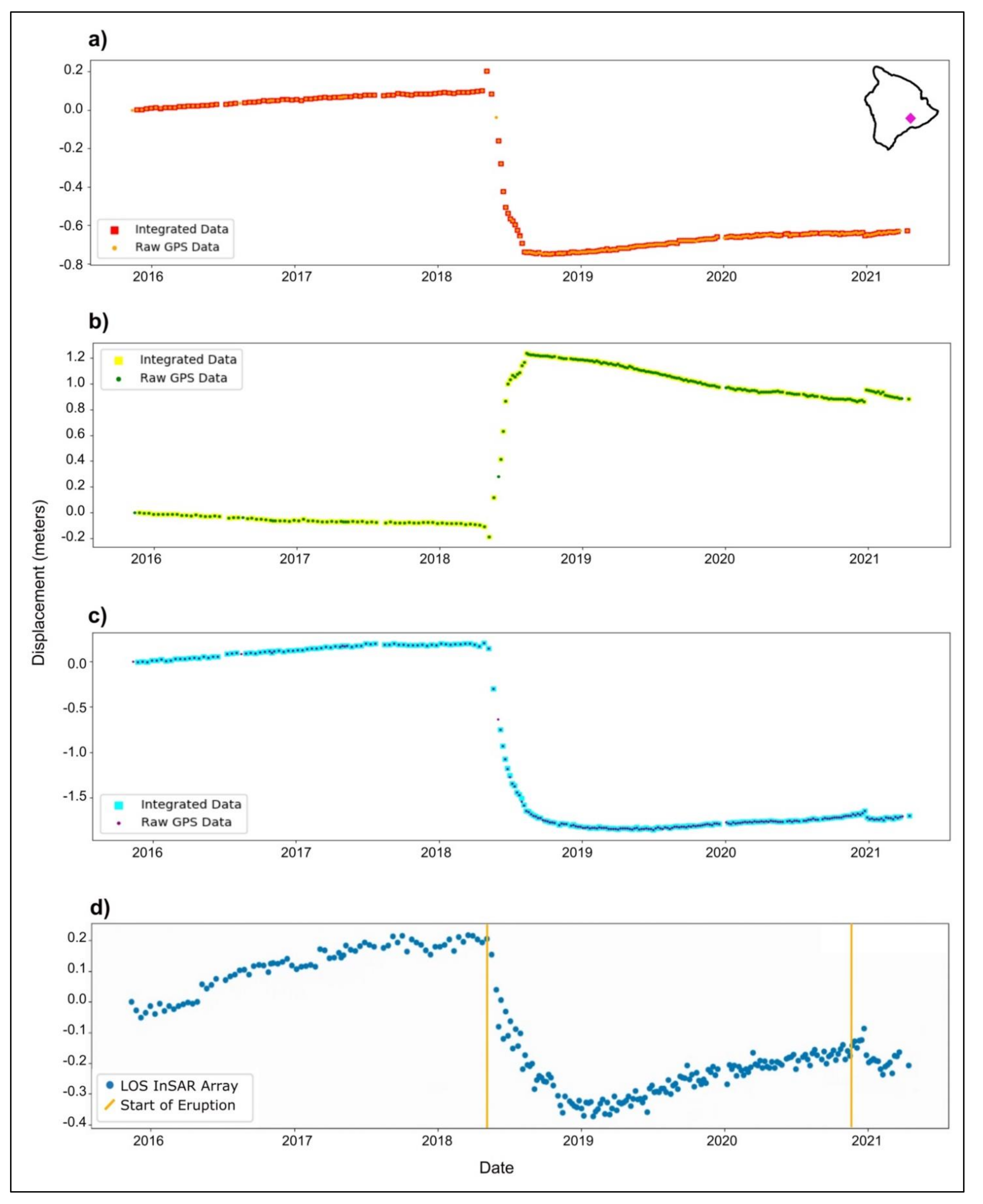
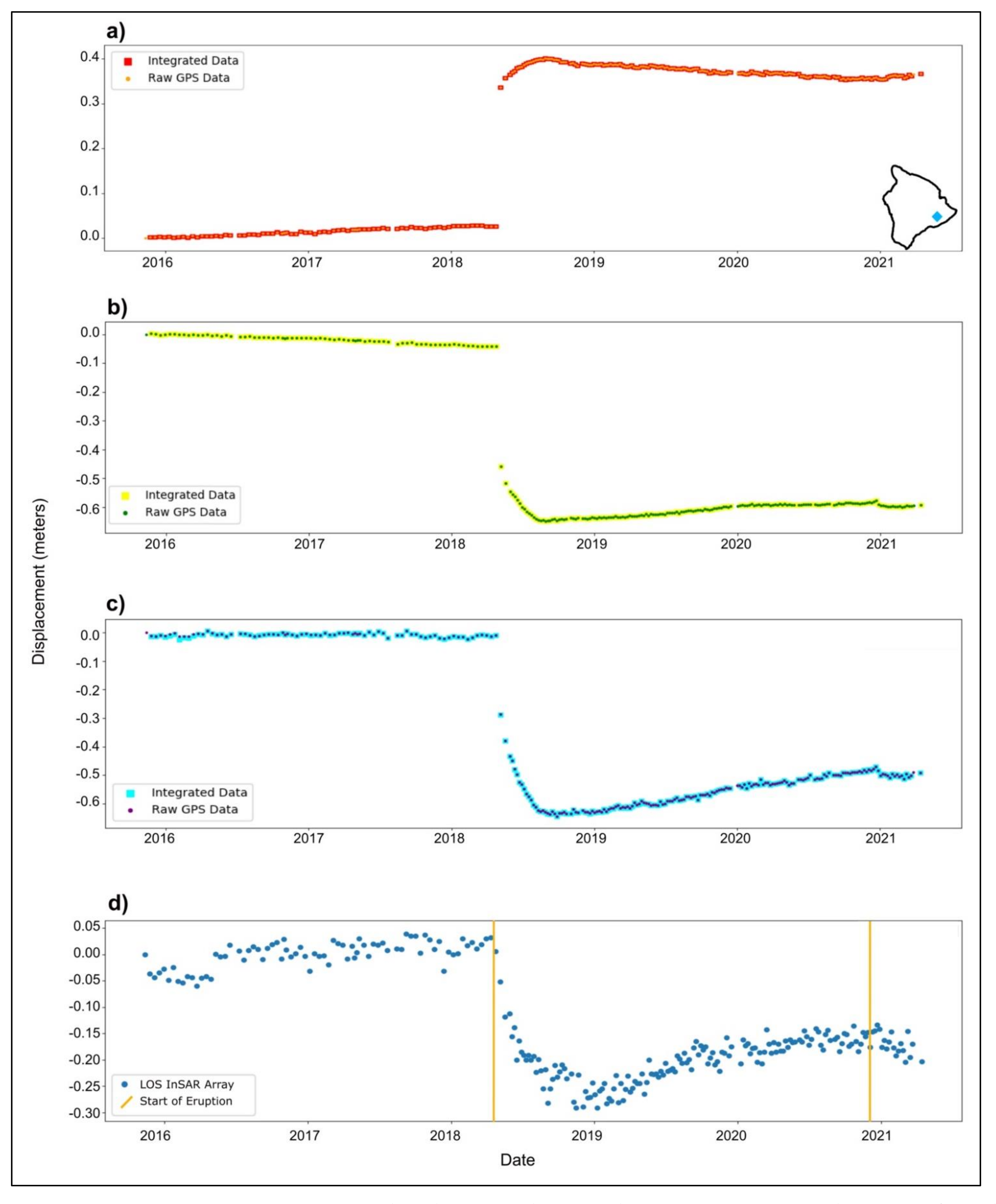
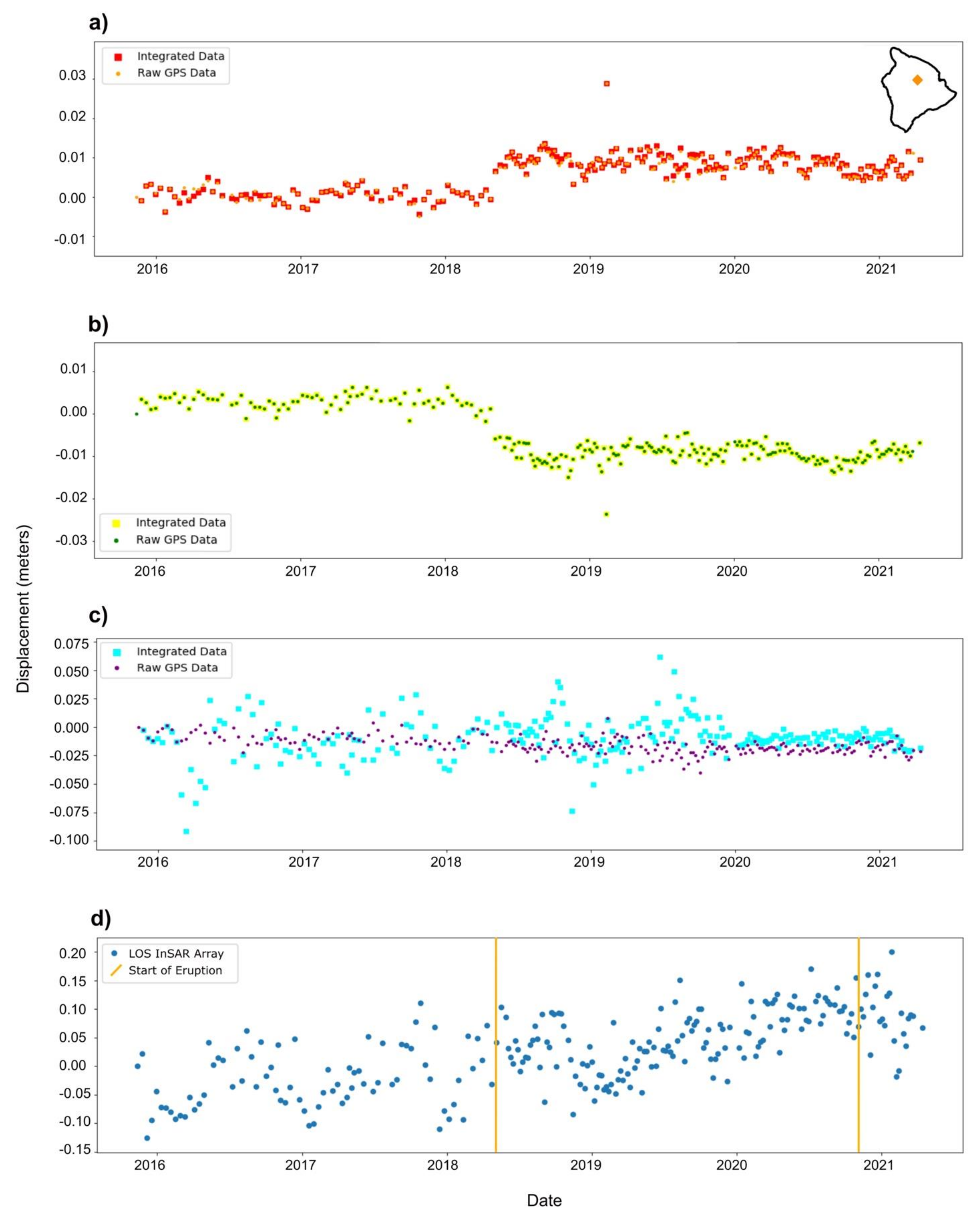
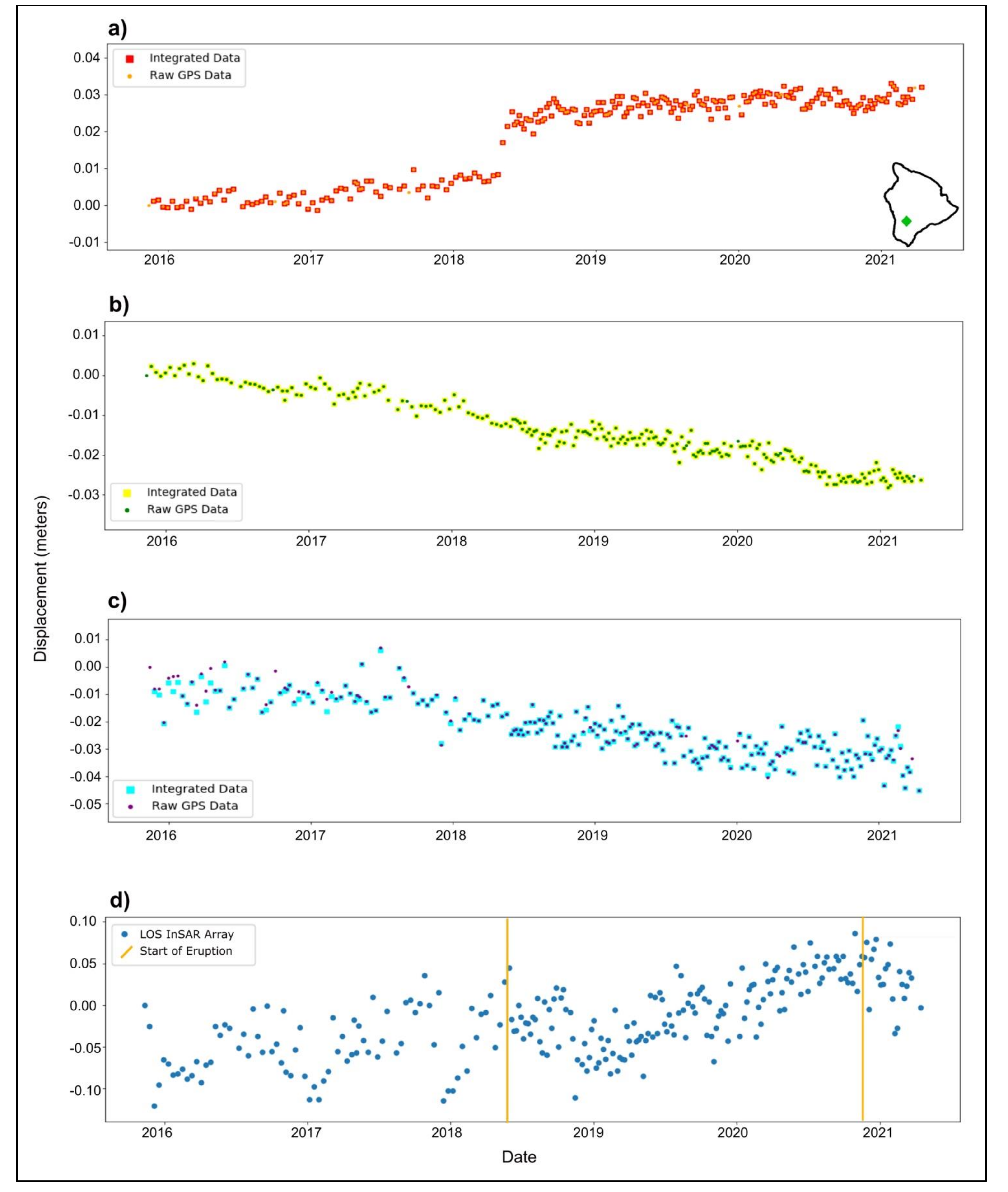
3.2. Plotted Time Series

In addition to generating the assimilated displacement maps, we present time series at four locations within the image where the GNSS stations overlap with a corresponding DInSAR pixel coordinate. These stations are strategically positioned across the island and include both active and relatively stable regions. Figure 8, Figure 9, Figure 10 and Figure 11 present the DInSAR+GNSS integrated time series at CRIM, NUPM, MKEA, and BLBP GNSS stations, respectively. We compare each component of motion from the integrated dataset with the raw GNSS time series and LOS DInSAR time series. These graphs depict the ground movement of a single point at every time-step of the series and record the surface response of that specific location to the two volcanic eruptions. The selected GNSS stations monitor a mixture of the most and least active regions of Hawaii and span a large spatial extent of the island. Similar to the 3D displacement maps, these individual time series provide researchers with a comprehensive study of surface deformation through time. By comparing the integrated product against the original GNSS time series, we find that information in the horizontal direction is slightly improved and information in the vertical direction is significantly enhanced once fused with LOS DInSAR measurements. The plotted time series provide additional insight into the temporal behavior at any given location.
The CRIM station (Figure 8) is located at the summit of Hawaii’s most active volcano, Kilauea, along the southern rim of the Halema’uma’u crater (purple diamond, Figure 1). At the CRIM station, the integrated results align nicely with the raw GNSS data. Over the period of time leading up to the 2018 eruption (November 2015 through May 2018), the ground at the CRIM station experienced 15.56 cm of horizontal motion to the southeast and 22 cm of uplift. The May 4 Mw 6.9 earthquake jolted the ground 11.4 cm further southeast and uplifted suddenly by 2 cm before volcanic activity dominated the signal. From the eruption itself, the ground moved 1.65 m northwest and subsided almost 2 m before it began a period of steady recovery at the beginning of 2019. Between January 2019 and December 2020, the CRIM station recovered 41 cm of south-southeast motion and uplifted approximately 20 cm from its lowest surface height. Finally, we observed another smaller jolt of ground motion 10.44 cm northeast and 10 cm down in response to the 20 December 2020 summit eruption.
The NUPM station (Figure 9) is positioned at the Puʻu ʻŌʻō volcano (blue diamond, Figure 1), which connects with the ERZ. We present plotted time series from this location to show the sudden displacement from the May 4 Mw 6.9 earthquake. The ground at NUPM stayed relatively stable between November 2015 and May 2018, leading up to the volcanic eruption, with ~4.5 cm southeast motion and stable (+/−1 cm) fluctuations in the vertical direction. Suddenly, the signal broke 58.83 cm southeast and 28 cm downward. Volcanic activity took over the signal and continued over the next couple of months, adding 20.88 cm of horizontal motion to the southeast (net total of 79.71 cm) and another 38 cm of subsidence (net total of 66 cm) before entering a state of ground recovery. Leading to the December 2020 summit eruption, the ground at the NUPM station recovered ~8.95 cm to the northwest and regained 17 cm of uplift. The summit eruption was slightly detectable at this location, having recorded 2 cm of motion to the northeast.
The MKEA station (Figure 10) lies along the southeastern flank of the dormant volcano, Mauna Kea (orange diamond, Figure 1). Data from November 2015 to January 2020 at the MKEA station was associated with the highest uncertainty values throughout this study. In the horizontal directions, the integrated dataset agreed nicely with the GNSS data; however, in the vertical orientation, the data trended more with the DInSAR time series results between 2015 and 2019. In January 2020, HVO reported an instrumental dome replacement, after which the variability in the integrated signal tightened, yet still deviated slightly (~1 cm) from the raw GNSS data. This time series provides an important example of the GNSS dataset with the highest error used in this study and demonstrates how combing the GNSS data with DInSAR also keeps a system of checks and balances of the integrated system. Even with high uncertainty, we could distinguish a 2.5 cm trend southeastward during the 2018 eruption.
The scatter observed in the DInSAR data, and the integrated results in the up direction in Figure 10 are partially due to the fact that the GPS data is at a single, isolated point, while the DInSAR results average the value of deformation over a 100 × 100 m2 pixel. The DInSAR values may also contain small amounts of residual tropospheric noise. Examination of the MKEA station (Figure 10), which is associated with the highest uncertainty measurements from the array of 48 GNSS stations, illustrates how the integrated dataset deviates significantly from the GNSS data in the up direction. Motions in the east-west and north-south directions are slightly more constrained, and motion in the up-down direction is significantly transformed after combining the DInSAR and GNSS datasets together. The integration algorithm weighs the DInSAR time series more than the GNSS data based on the errors of the individual datasets (see Supplemental Material).
Finally, the BLBP GNSS site (Figure 11) is situated over an area of comparatively stable ground along the southwestern part of the island, where relatively low activity was maintained over the duration of our time series (green diamond, Figure 1). Leading up to the 2018 volcanic eruption, the ground at BLBP experienced approximately 1 cm of eastward motion, while remaining within ± 4 mm of motion in the north-south direction. At the time of the 2018 eruption, the BLBP station moved ~12 cm to the east, remained steady in its north-south component of motion, and unclearly moved in the up-down direction. Nevertheless, over the entire time series, we detected that the ground at the BLBP station moved a total of ~3 cm to the southeast, and ~4 cm of subsidence occurred between November 2015 and April 2021.

4. Discussion

The 2018 event at Kilauea volcano was the largest caldera collapse and most effusive volcanic eruption in Hawaii within the past 200 years [26,48,49,50,51]. Combining high-quality geodetic datasets, such as DInSAR and GNSS, resulted in detailed observations and precise measurements regarding the development and evolution of volcanic events.
The median uncertainty associated with the LOS DInSAR dataset was 6.60 mm, and the average was 6.54 mm. The maximum uncertainty associated with our LOS DInSAR displacement maps came from the final cumulative time slice and was equal to 1.03 cm. This uncertainty considers errors estimated from the DEM, orbital, and atmospheric corrections applied during processing.
The median errors associated with the raw GNSS data in the east, north, and up directions were 0.81 mm, 0.74 mm, and 3.27 mm, respectively. The corresponding maximum uncertainties associated with the raw GNSS data in the east, north, and up directions were 7.63 mm, 3.28 mm, and 9.65 mm. For direct comparison with the LOS DInSAR data, the converted LOS vector component of the raw GNSS data took on a maximum uncertainty of 1.27 cm.
Integrated uncertainties were combined from the raw DInSAR and GNSS sigma values using the same methodology as the real data (see Supplementary Material Equations S1–S8). Maximum integrated uncertainty in the LOS component of motion was 7.93 mm. When generating the 3D displacement maps, however, the error introduced from using the kriging algorithm and interpolating over undefined points in the spatial field must also be included, and in doing so, resulting in increased maximum uncertainties in the east, north, and up directions of 7.07 cm, 5.82 cm, and 5.71 cm, respectively.
At a single pixel, where kriging interpolation was not applied, the accuracy of our deformation measurements improved. For example, at the corresponding pixel where the CRIM GNSS station is situated, the median uncertainties for the raw GNSS time series data in the east, north, and up directions of motion were 0.77 mm, 0.70 mm, and 3.06 mm, respectively. The raw LOS DInSAR time series at this specific location had a median uncertainty of 1.99 mm. By integrating the two geodetic datasets together, the fused dataset had an improved median uncertainty of 0.76 mm, 0.70 mm, and 1.95 mm in the east, north, and up directions. Further analyses of the errors associated with each dataset are available in the Supplementary Material.
Many other studies have utilized geodetic remote sensing techniques to better understand magmatic systems and volcanic eruptive history. Our raw interferometric products and LOS displacement values are consistent with those produced by the USGS HVO and European Space Agency, also processed with GMTSAR software with Snaphu phase unwrapping [52]. Furthermore, our results extend further evidence of the 62 summit collapse events between May 16 and August 2, reported by HVO. Another study by [50] used raw GNSS and DInSAR measurements from Hawaii as input for multi-reservoir conceptual models to quantitatively constrain the hydraulic connectivity between magmatic systems. By exploiting high-quality geodetic data, they learned that the Halema’uma’u magmatic reservoir is distinct from the South Caldera reservoir and that the ERZ is being fed simultaneously by both chambers. Our LOS inflation and deflation patterns over Kilauea and the ERZ agreed with their observations derived from descending interferograms from November 2018 through March 2019. Lundgren et al. [51] also used airborne InSAR measurements from the Glacier and Ice Surface Topography Interferometer (GLISTIN-A) instrument over Hawaii to measure the bulk volume of subaerial lava flows between 18 May and 15 September 2018. They found that 0.593 +/−0.011 km3 sourced from the Lower ERZ and −0.836 +/−0.002 km3 of material resulted from the summit collapse. Finally, a study at Piton de la Fournaise, France, used four interferograms to determine the displacement source and a temporal inversion of GNSS data to describe the dynamics of magmatic propagation [53].
These examples show the broad, interdisciplinary applications that come from a mix of DInSAR and GNSS monitoring over volcanic regions and further support the relevance and benefits of this study. A more accurate, fused dataset creates potential for improved volumetric analysis during large events, enhanced volcanic source modeling and mapping of magma chamber geometries or subsurface transport channels, and may provide a better means to forecast initial eruption sites or potential lava flow pathways along the surface.

5. Conclusions and Upcoming Work

Geodetic datasets such as DInSAR and GNSS time series contain valuable information for earth scientists. These data are particularly useful in analyzing the long-term evolution of volcanic systems. When integrated together, they deliver improved, more constrained estimates of 3D motions of the Earth’s surface. Inflation estimates such as that detected in our integrated time series prior to both eruptions are useful for hazard response purposes and applications and underline the importance of deformation monitoring in volcanic regions. The methods performed here can be applied to other regions in the world and can be easily adapted to different volcanic systems.
The integrated 3D displacement maps and associated time series provided new estimates and details of the spatial and temporal dynamics of the 2018 Hawaiian eruption. In conjunction with seismic, tide gauge, gas emission, and thermal datasets, the individual InSAR and GNSS time series and the combined results presented here will be streamed through machine learning algorithms capable of identifying pixels or clusters of pixels that exhibit anomalous movement. This will facilitate the detection and analysis of precursor motion and can be used to inform early warning systems. Eventually, the system will run continuously, providing researchers with large streams of historic or near real-time data from an array of geodetic sensors.
With a continuous, scalable, near real-time data streaming architecture in place, the combined data will contribute to the early detection of major geophysical events such as volcanic eruptions and improve our understanding of the fundamental processes involved over the locations of interest. The fused dataset can be used to improve volcanic modeling systems, using the long-term surface response to map the subsurface magmatic plumbing system. The results presented here also have additional detailed insight into earthquake dynamics, and further research may lead to the distinction or isolation of certain geophysical phenomena within the signal. Finally, the application of machine learning algorithms to these datasets will improve our understanding of the connections between these volcanoes or how activity at one location may have implications for potential activity at another and be critical inputs for early warning applications. These results will provide researchers with better methods in real-time or near real-time to monitor volcanic regions and evaluate resulting surface deformations with millimeter precision, ultimately advancing scientific discovery and benefitting efforts to further protect human life and property.

Supplementary Materials

The following are available online at https://www.mdpi.com/article/10.3390/rs14030784/s1, Supplementary List S1: 250 descending Sentinel-1 A/B SLC image IDs used in this study from Path 87 Frame 526 between 23 November 2015–13 April 2021; Supplementary List S2: List of 694 (671 successful) interferometric image date pairs crated from Supplementary List S1 using GMT5SAR software and allowing a maximum of 35 days between images; Figures S1–S3: Comparison of integrated, plotted time series results in the ITRF-14 reference frame for CRIM, MKEA, and BLBP GNSS stations, respectively; Equations S1–S8: Integrating Geodetic Datasets and Inversion Processes; Figure S4: Raw GNSS uncertainty results; Figure S5: Variance associated with the Kriging interpolation used to generate the GPS displacement maps; Figure S6: Uncertainties associated with the cumulative, integrated DInSAR+GNSS results; Figures S7–S10: Integrated uncertainty for the plotted time series at the overlapping pixel location for CRIM, NUPM, MKEA, BLBP GNSS stations, respectively.

Author Contributions

Conceptualization, B.C., M.B.-S., K.T.; methodology, B.C., M.B.-S., K.T.; software, B.C., M.B.-S.; validation, B.C., M.B.-S., K.T., C.M.; formal analysis, B.C., M.B.-S., K.T., C.M.; investigation, B.C.; resources, B.C., M.B.-S., K.T., C.M.; data curation, B.C.; writing—original draft preparation, B.C.; writing—review and editing, B.C., K.T.; visualization, B.C.; supervision, B.C., M.B.-S., K.T., C.M.; project administration, K.T., C.M.; funding acquisition, K.T., C.M. All authors have read and agreed to the published version of the manuscript.

Funding

This research was funded by NSF Grant No. 1835566, Grant No. 1835791, Collaborative Research:Framework:Data:NSCI:HDR:GeoSCIFramework:Scalable Real-Time Streaming Analytics and Machine Learning for Geoscience and Hazards Research.

Institutional Review Board Statement

Not applicable.

Informed Consent Statement

Not applicable.

Data Availability Statement

GNSS processed time series are freely available and downloadable through the Nevada Geodetic Laboratory (http://geodesy.unr.edu/ (accessed on 3 April 2021)). Data stations are maintained by the USGS HVO [23,24], and data are archived and distributed by the UNAVCO GAGE facility. Sentinel-1 A/B DInSAR imagery is also freely available and downloadable through the Alaska Satellite Facility Vertex Portal [22] (https://search.asf.alaska.edu/#/ (accessed on 15 April 2021)). In the future, all products in this paper and produced as part of the project will be available under the GeoSciFramework project website (https://www.unavco.org/projects/major-projects/earthcube/geosciframework/geosciframework.html (accessed on 5 August 2021)). For DInSAR Data used in this study: Copernicus Sentinel data [2015–2021]. Retrieved from ASF DAAC [acquired 01 February 2021], processed by ESA. For Atmospheric Data used in this study: GACOS is supported by NERC through the center for seismic, volcanic, and tectonic observation and modeling (comet, Ref.: come30001) and LICs (Ref. Ne/k010794/1) and esa-most dragon-4 (Ref. 32244). We recognize the European Centre for medium-range weather forecasts (ECMWF) for its high-resolution tropospheric products. For GNSS Stations used in this study: Station MKEA is operated by the Jet Propulsion Laboratory and UNAVCO with NASA funding. Data are freely available from the NASA Crustal Dynamics Date Information System (CDDIS). For the following stations: ANIP, ALAL, APNT, HLNA, KAON, KHKU, KNNE, MKEA, MLES, MLRD, PAT3, PHAN, PIIK, PUH2, PUKA, RADF, and SLPC, citation: OBSERVER: Benjamin Brooks, AGENCY: Pacific GPS Facility, U of Hawaii/and Blewit et al. (2018). The following information obtained from UNAVCO’s online DOI system: (https://www.unavco.org/data/doi/search/search.html) (accessed on 4 April 2021). Hawaii GPS Network-AHUP-Ahua P.S. Start: 30-May-1999, End: 16-May-2019 Segall, Paul, Miklius, Asta, 1999. Hawaii GPS Network-AHUP-Ahua P.S., UNAVCO, GPS/GNSS Observations Dataset, https://doi.org/10.7283/T5ST7MW0) (accessed on 4 April 2021). Hawaii GPS Network-AINP-Ainapo P.S. Start: 08-Oct-2002, End: 16-May-2019, Miklius, Asta, 2002, Hawaii GPS Network-AINP-Ainapo P.S., UNAVCO, GPS/GNSS Observations Dataset, https://doi.org/10.7283/T5348HMF) (accessed on 4 April 2021). Hawaii GPS Network-ALEP-ALEA Permanent P.S. Start: 15-Jul-2004, End: 15-May-2019, Miklius, Asta, 2004, Hawaii GPS Network-ALEP-ALEA Permanent P.S., UNAVCO, GPS/GNSS Observations Dataset, https://doi.org/10.7283/T52805VG) (accessed on 4 April 2021). Hawaii GPS Network-BLBP-Bluebird P.S., Start: 08-Jun-2004, End: 15-May-2019, Miklius, Asta, 2004, Hawaii GPS Network-BLBP-Bluebird P.S., UNAVCO, GPS/GNSS Observations Dataset, https://doi.org/10.7283/T5FF3QKS) (accessed on 4 April 2021). Hawaii GPS Network-BYRL-Byrons Ledge P.S., Start: 27-Feb-2006, End: 16-May-2019, Miklius, Asta, 2006, Hawaii GPS Network-BYRL-Byrons Ledge P.S., UNAVCO, GPS/GNSS Observations Dataset, https://doi.org/10.7283/T5NZ85W4) (accessed on 4 April 2021). Hawaii GPS Network-CNPK-Cone Peak P.S., Start: 25-Jun-2008, End: 16-May-2019, Miklius, Asta, 2008, Hawaii GPS Network-CNPK-Cone Peak P.S., UNAVCO, GPS/GNSS Observations Dataset, https://doi.org/10.7283/T5N014RM) (accessed on 4 April 2021). Hawaii GPS Network-CRIM-Crater Rim P.S., Start: 06-Jun-2008, End: 16-May-2019, Miklius, Asta, 2008, Hawaii GPS Network-CRIM-Crater Rim P.S., UNAVCO, GPS/GNSS Observations Dataset, https://doi.org/10.7283/T5RR1WGN) (accessed on 4 April 2021). Hawaii GPS Network-ELEP-Ele‘ele P.S., Start: 09-Dec-2000, End: 15-May-2019, Miklius, Asta, 2000, Hawaii GPS Network-ELEP-Ele‘ele P.S., UNAVCO, GPS/GNSS Observations Dataset, https://doi.org/10.7283/T5BP011P) (accessed on 4 April 2021). Hawaii GPS Network-GOPM-Goat P.S., Start: 30-May-1999, End: 16-May-2019, Segall, Paul, Miklius, Asta, 1999, Hawaii GPS Network-GOPM-Goat P.S., UNAVCO, GPS/GNSS Observations Dataset, https://doi.org/10.7283/T5P26W50) (accessed on 4 April 2021). Hawaii GPS Network-HOLE-Holei P.S., Start: 30-May-1999, End: 16-May-2019, Segall, Paul, Miklius, Asta, 1999, Hawaii GPS Network-HOLE-Holei P.S., UNAVCO, GPS/GNSS Observations Dataset, https://doi.org/10.7283/T5RV0KR5) (accessed on 4 April 2021). Hawaii GPS Network-JCUZ-Pu‘u ‘O‘o JCUZ P.S., Start: 06-Jul-2007,End: 16-May-2019, Miklius, Asta, 2007, Hawaii GPS Network-JCUZ-Pu‘u ‘O‘o JCUZ P.S., UNAVCO, GPS/GNSS Observations Dataset, https://doi.org/10.7283/T5416V92) (accessed on 4 April 2021). Hawaii GPS Network-JOKA-Jonika P.S., Start: 03-Oct-2007, End: 16-May-2019, Miklius, Asta, 2007, Hawaii GPS Network-JOKA-Jonika P.S., UNAVCO, GPS/GNSS Observations Dataset, https://doi.org/10.7283/T58P5XR4) (accessed on 4 April 2021). Hawaii GPS Network-KAEP-Kaena Point P.S., Start: 30-May-1999, End: 16-May-2019, Segall, Paul, Miklius, Asta, 1999, Hawaii GPS Network-KAEP-Kaena Point P.S., UNAVCO, GPS/GNSS Observations Dataset, https://doi.org/10.7283/T5J964D6) (accessed on 4 April 2021). Hawaii GPS Network-KAMO-Pu‘u Kamoamoa P.S., Start: 10-Aug-2007, End: 16-May-2019, Miklius, Asta, 2007, Hawaii GPS Network-KAMO-Pu‘u Kamoamoa P.S., UNAVCO, GPS/GNSS Observations Dataset, https://doi.org/10.7283/T5G73BXZ) (accessed on 4 April 2021). Hawaii GPS Network-KFAP-Kaoiki Fault P.S., Start: 16-Jul-2004, End: 16-May-2019, Miklius, Asta, 2004, Hawaii GPS Network-KFAP-Kaoiki Fault P.S., UNAVCO, GPS/GNSS Observations Dataset, https://doi.org/10.7283/T59P2ZV2) (accessed on 4 April 2021). Hawaii GPS Network-KOSM-KOSM P.S., Start: 01-Aug-1999, End: 16-May-2019, Segall, Paul, Miklius, Asta, 2000, Hawaii GPS Network-KOSM-KOSM P.S., UNAVCO, GPS/GNSS Observations Dataset, https://doi.org/10.7283/T59S1P23) (accessed on 4 April 2021). Hawaii GPS Network-KTPM-Kalapana Trail P.S., Start: 30-May-1999, End: 16-May-2019, Segall, Paul, Miklius, Asta, 1999, Hawaii GPS Network-KTPM-Kalapana Trail P.S., UNAVCO, GPS/GNSS Observations Dataset, https://doi.org/10.7283/T5DJ5CN1) (accessed on 4 April 2021). Hawaii GPS Network-MANE-Mauka Kipuka Nene P.S., Start: 30-May-1999, End: 16-May-2019, Segall, Paul, Miklius, Asta, 1999, Hawaii GPS Network-MANE-Mauka Kipuka Nene P.S., UNAVCO, GPS/GNSS Observations Dataset, https://doi.org/10.7283/T5513W86) (accessed on 4 April 2021). Hawaii GPS Network-MKAI-Makai Makaopuhi P.S., Start: 09-Jul-2010, End: 16-May-2019, Miklius, Asta, 2010, Hawaii GPS Network-MKAI-Makai Makaopuhi P.S., UNAVCO, GPS/GNSS Observations Dataset, https://doi.org/10.7283/T57S7M01) (accessed on 4 April 2021), Hawaii GPS Network-MLCC-Mauna Loa Cinder Cone P.S., Start: 02-Jul-2004, End: 15-May-2019, Miklius, Asta, 2004, Hawaii GPS Network-MLCC-Mauna Loa Cinder Cone P.S., UNAVCO, GPS/GNSS Observations Dataset, https://doi.org/10.7283/T56W989D) (accessed on 4 April 2021). Hawaii GPS Network-MLSP-Mauna Loa Summit P.S., Start: 09-Dec-2000, End: 16-May-2019, Miklius, Asta, 2000, Hawaii GPS Network-MLSP-Mauna Loa Summit P.S., UNAVCO, GPS/GNSS Observations Dataset, https://doi.org/10.7283/T5K64G9H) (accessed on 4 April 2021). Hawaii GPS Network-MMAU-Mauka Makaopuhi P.S., Start: 09-Jul-2010, End: 16-May-2019, Miklius, Asta, 2010, Hawaii GPS Network-MMAU-Mauka Makaopuhi P.S., UNAVCO, GPS/GNSS Observations Dataset, https://doi.org/10.7283/T5CF9NBG) (accessed on 4 April 2021). Hawaii GPS Network-MOKP-Moku‘aweoweo P.S., Start: 09-Dec-2000, End: 16-May-2019, Miklius, Asta, 2000, Hawaii GPS Network-MOKP-Moku‘aweoweo P.S., UNAVCO, GPS/GNSS Observations Dataset, https://doi.org/10.7283/T5TQ5ZS9) (accessed on 4 April 2021). Hawaii GPS Network-NPOC-North Pu‘u P.S., Start: 05-Jul-2007, End: 16-May-2019, Miklius, Asta, 2007, Hawaii GPS Network-NPOC-North Pu‘u P.S., UNAVCO, GPS/GNSS Observations Dataset, https://doi.org/10.7283/T5QR4VB8) (accessed on 4 April 2021). Hawaii GPS Network-NUPM-Kane Nui O Hamo P.S., Start: 30-May-1999, End: 16-May-2019, Segall, Paul, Miklius, Asta, 1999, Hawaii GPS Network-NUPM-Kane Nui O Hamo P.S., UNAVCO, GPS/GNSS Observations Dataset, https://doi.org/10.7283/T58S4MZR) (accessed on 4 April 2021). Hawaii GPS Network-OUTL-Outlet P.S., Start: 18-April-2008, End: 16-May-2019, Miklius, Asta, 2008, Hawaii GPS Network-OUTL-Outlet P.S., UNAVCO, GPS/GNSS Observations Dataset, https://doi.org/10.7283/T5WH2N7T) (accessed on 4 April 2021). Hawaii GPS Network-PMAU-Pu‘u Ma‘au P.S., Start: 27-Oct-2006, End: 16-May-2019, Miklius, Asta, 2006, Hawaii GPS Network-PMAU-Pu‘u Ma‘au P.S., UNAVCO, GPS/GNSS Observations Dataset, https://doi.org/10.7283/T5DF6PFD) (accessed on 4 April 2021). Hawaii GPS Network-STEP-Mauna Loa Observatory P.S., Start: 12-Oct-2002, End: 15-May-2019, Miklius, Asta, 2002, Hawaii GPS Network-STEP-Mauna Loa Observatory P.S., UNAVCO, GPS/GNSS Observations Dataset, https://doi.org/10.7283/T5PZ572C) (accessed on 4 April 2021). Hawaii GPS Network-TOUO-Tube Ouo P.S., Start: 10-Jul-2004, End: 15-May-2019, Miklius, Asta, 2004, Hawaii GPS Network-TOUO-Tube Ouo P.S., UNAVCO, GPS/GNSS Observations Dataset, https://doi.org/10.7283/T55X275K) (accessed on 4 April 2021), Hawaii GPS Network-UWEV-Uwekahuna Vault P.S., Start: 30-May-1999, End: 16-May-2019, Segall, Paul, Miklius, Asta, 1999, Hawaii GPS Network-UWEV-Uwekahuna Vault P.S., UNAVCO, GPS/GNSS Observations Dataset, https://doi.org/10.7283/T51C1TXB) (accessed on 4 April 2021).

Conflicts of Interest

The authors declare no conflict of interest. The funders had no role in the design of the study; in the collection, analyses, or interpretation of data; in the writing of the manuscript, or in the decision to publish the results.

References

  1. Aiuppa, A.; Moretti, R.; Cinzia, F.; Giudice, G.; Gurrieri, S.; Liuzzo, M.; Papale, P.; Shinohara, H.; Valenza, M. Forecasting Etna eruptions by real-time observation of volcanic gas composition. Geology 2007, 35, 1115–1118. [Google Scholar] [CrossRef]
  2. Anantrasirichai, N.; Biggs, J.; Albino, F.; Hill, P.; Bull, D. Application of machine learning to classification of volcanic deformation in routinely generated InSAR data. J. Geophys. Res. Solid Earth 2018, 123, 6592–6606. [Google Scholar] [CrossRef] [Green Version]
  3. Bebbington, M.S. Long-term forecasting of volcanic explosivity. Geophys. J. Int. 2014, 197, 1500–1515. [Google Scholar] [CrossRef]
  4. Marzocchi, W.; Bebbington, M.S. Probabilistic eruption forecasting at short- and long-time scales. Bull. Volcanol. 2012, 74, 1777–1805. [Google Scholar] [CrossRef]
  5. Phillipson, G.; Sobradelo, R.; Gottsmann, J. Global volcanic unrest in the 21st century: An analysis of the first decade. J. Volcanol. Geotherm. Res. 2013, 264, 183–196. [Google Scholar] [CrossRef]
  6. Potter, S.H.; Scott, B.J.; Fearnley, C.J.; Leonard, G.S.; Gregg, C.E. Challenges and benefits of standardising early warning system. In Observing the Volcano World; Fearnley, C.J., Bird, D.K., Haynes, K., McGuire, W.J., Jolly, G., Eds.; Advances in Volcanology (An Official Book Series of the International Association of Volcanology and Chemistry of the Earth’s Interior). Springer: New York, NY, USA, 2017. [Google Scholar] [CrossRef] [Green Version]
  7. Rouwet, D.; Sandri, L.; Marzocchi, W.; Gottsmann, J.; Selva, J.; Tonini, R.; Papale, P. Recognizing and tracking volcanic hazards related to non-magmatic unrest: A review. J. Appl. Volcanol. 2014, 3, 17. [Google Scholar] [CrossRef] [Green Version]
  8. Stix, J. Understanding fast and slow unrest at volcanoes and implications for eruption forecasting. Front. Earth Sci. 2018, 6, 2018. [Google Scholar] [CrossRef] [Green Version]
  9. Kelevitz, K.; Tiampo, K.F.; Corsa, B.D. Improved real-time natural hazard monitoring automated DInSAR time series. Remote Sens. 2021, 13, 867. [Google Scholar] [CrossRef]
  10. Chen, K.; Smith, J.D.; Avouac, J.-P.; Liu, Z.; Song, Y.T.; Gualandi, A. Triggering of the Mw 7.2 Hawaii earthquake of 4 May 2018 by a dike intrusion. Geophys. Res. Lett. 2019, 46, 2503–2510. [Google Scholar] [CrossRef]
  11. Derauw, D.; d’Oreye, N.; Jaspard, M.; Caselli, A.; Samsonov, S. Ongoing automated ground deformation monitoring of Domuyo—Laguna del Maule area (Argentina) using Sentinel-1 MSBAS time series: Methodology description and first observations for the period 2015–2020. J. South Am. Earth Sci. 2020, 104, 102850. [Google Scholar] [CrossRef]
  12. Samsonov, S.; Tiampo, K. Analytical optimization of DInSAR and GPS dataset for derivation of three-dimensional surface motion. IEEE Geosci. Remote Sens. Lett. 2006, 3, 107–111. [Google Scholar] [CrossRef]
  13. Samsonov, S.V.; Feng, W.; Fialko, Y. Subsidence at cerro prieto geothermal field and postseismic slip along the indiviso fault from 2011 to 2016 RADARSAT-2 DInSAR time series analysis. Geophys. Res. Lett. 2017, 44, 2716–2724. [Google Scholar] [CrossRef]
  14. Tilling, R.I. Volcanic hazards and early warning. In Encyclopedia of Complexity and Systems Science; Meyers, R., Ed.; Springer: New York, NY, USA, 2009. [Google Scholar] [CrossRef]
  15. Valade, S.; Ley, A.; Massimetti, F.; D’Hondt, O.; Laiolo, M.; Coppola, D.; Loibl, D.; Hellwich, O.; Walter, T.R. Towards global volcano monitoring using multisensor sentinel missions and artificial intelligence: The MOUNTS monitoring system. Remote Sens. 2019, 11, 1528. [Google Scholar] [CrossRef] [Green Version]
  16. Lundgren, P.; Girona, T.; Bato, M.G.; Realmut, V.J.; Samsonov, S.; Cardona, C.; Franco, L.; Gurrola, E.; Aivazis, M. The dynamics of large silicic systems from satellite remote sensing observations: The intriguing case of Domuyo volcano, Argentina. Sci. Rep. 2020, 10, 11642. [Google Scholar] [CrossRef]
  17. Ji, P.; Lv, X.; Yao, J.; Sun, G. A new method to obtain 3-D surface deformations from InSAR and GNSS data with genetic algorithm and support vector machine. IEEE Geosci. Remote Sens. Lett. 2022, 19, 1–5. [Google Scholar] [CrossRef]
  18. Samsonov, S.; Tiampo, K.; Rundle, J.; Li, Z. Application of DInSAR-GPS optimization for derivation of fine scale surface motion maps of southern California. IEEE Trans. Geosci. Remote Sens. 2007, 45, 512–522. [Google Scholar] [CrossRef] [Green Version]
  19. Samsonov, S.; Tiampo, K.; Rundle, J. Application of DInSAR-GPS optimization for derivation of three-dimensional surface motion of southern California region along the San Andreas fault. Comput. Geosci. 2008, 34, 503–514. [Google Scholar] [CrossRef]
  20. Vollrath, A.; Zucca, F.; Bekaert, D.; Bonforte, A.; Guglielmino, F.; Hooper, A.J.; Stramondo, S. Decomposing DInSAR time-series into 3-D in combination with GPS in the case of low strain rates: An application to the Hyblean Plateau, Sicily, Italy. Remote Sens. 2017, 9, 33. [Google Scholar] [CrossRef] [Green Version]
  21. Copernicus Sentinel-1 data 2015–2021, retrieved from ASF DAAC 23-04-2021, processed by ESA. Available online: https://asf.alaska (accessed on 15 April 2021).
  22. Blewitt, G.; Hammond, W.C.; Kreemer, C. Harnessing the GPS data explosion for interdisciplinary science. Eos 2018, 99, 485. [Google Scholar] [CrossRef]
  23. Miklius, A. Hawaii GPS Network-CNPK-Cone Peak P.S. The GAGE Facility operated by UNAVCO, Inc., GPS/GNSS Observations Dataset. 2008. Available online: https://doi.org/10.7283/T5N014RM (accessed on 5 October 2021). [CrossRef]
  24. USGS.gov. December 2020–May 2021 Eruption. Available online: https://www.usgs.gov/volcanoes/kilauea/december-2020-may-2021-eruption?qt-science_support_page_related_con=0#qt-science_support_page_related_con (accessed on 5 October 2021).
  25. USGS.gov. Available online: https://volcanoes.usgs.gov/volcanoes/Kilauea/ (accessed on 5 October 2021).
  26. Patrick, M.R.; Houghton, B.F.; Anderson, K.R.; Poland, M.P.; Montgomery-Brown, E.; Johanson, I.; Thelen, W.; Elias, T. The cascading origin of the 2018 Kīlauea eruption and implications for future forecasting. Nat. Commun. 2020, 11, 5646. [Google Scholar] [CrossRef]
  27. Sandwell, D.; Mellors, R.; Tong, X.; Wei, M.; Wessel, P. Open radar interferometry software for mapping surface deformation. Eos Trans. AGU 2011, 92, 234. [Google Scholar] [CrossRef] [Green Version]
  28. Sandwell, D.; Mellors, R.; Tong, X.; Wei, M.; Wessel, P. GMTSAR: An InSAR Processing System Based on Generic Mapping Tools; UC San Diego Scripps Institution of Oceanography: La Jolla, CA, USA, 2011; Available online: http://escholarship.org/uc/item/8zq2c02m (accessed on 1 October 2021).
  29. Berardino, P.; Fornaro, G.; Lanari, R.; Sansosti, E. A new algorithm for surface deformation monitoring based on small baseline differential SAR interferograms. IEEE Trans. Geosci. Remote Sens. 2002, 40, 2375–2383. [Google Scholar] [CrossRef] [Green Version]
  30. Doin, M.P.; Guillaso, S.; Jolivet, R.; Lasserre, C.; Lodge, F.; Ducret, G. Presentation of the small baseline NSBAS processing chain on a case example: The Etna deformation monitoring from 2003 to 2010 using Envisat data. In Proceedings of the ESA FRINGE 2011 Conference, Frascati, Italy, 19–23 September 2011. [Google Scholar]
  31. Zimmerman, D.; Pavlik, C.; Ruggles, A.; Armstrong, M.P. An experimental comparison of ordinary and universal kriging and inverse distance weighting. Math. Geol. 1999, 31, 375–390. [Google Scholar] [CrossRef]
  32. Matheron, G. Principles of geostatistics. Econ. Geol. 1963, 58, 1246–1266. [Google Scholar] [CrossRef]
  33. Moussouris, J. Gibbs and Markov random systems with constraints. J. Stat. Phys. 1974, 10, 11–33. [Google Scholar] [CrossRef]
  34. Johnson, C.W.; Lau, N.; Borsa, A. An assessment of GPS velocity uncertainty in California. Earth Space Sci. 2020, 8, e2020EA001345. [Google Scholar] [CrossRef]
  35. Wang, S.-Y.; Li, J.; Chen, J.; Hu, X.-G. Uncertainty assessments of load deformation from different GPS time series products, GRACE estimates and model predictions: A case study over Europe. Remote Sens. 2021, 13, 2765. [Google Scholar] [CrossRef]
  36. Chen, C.W.; Zebker, H.A. Phase unwrapping for large SAR interferograms: Statistical segmentation and generalized network model. IEEE Trans. Geosci. Remote Sens. 2002, 40, 1709–1719. [Google Scholar] [CrossRef] [Green Version]
  37. Agram, P.; Jolivet, R.; Riel, B.-V.; Simons, M.; Doin, M.; Lasserre, C.; Hetland, E.-A. GIAnT—Generic InSAR Analysis Toolbox, American Geophysical Union, Fall Meeting 2012, abstract id. G43A-0897. Available online: https://ui.adsabs.harvard.edu/abs/2012AGUFM.G43A0897A (accessed on 1 December 2021).
  38. Yu, C.; Penna, N.T.; Li, Z. Generation of real-time mode high-resolution water vapor fields from GPS observations. J. Geophys. Res. Atmos. 2017, 122, 2008–2025. [Google Scholar] [CrossRef]
  39. Yu, C.; Li, Z.; Penna, N.T. Interferometric synthetic aperture radar atmospheric correction using a GPS-based iterative tropospheric decomposition model. Remote Sens. Environ. 2018, 204, 109–121. [Google Scholar] [CrossRef]
  40. Yu, C.; Li, Z.; Penna, N.T.; Crippa, P. Generic atmospheric correction model for Interferometric Synthetic Aperture Radar observations. J. Geophys. Res. Solid Earth 2018, 123, 9202–9222. [Google Scholar] [CrossRef]
  41. Yu, C.; Li, Z.; Penna, N.T. Triggered afterslip on the southern Hikurangi subduction interface following the 2016 Kaikōura earthquake from InSAR time series with atmospheric corrections. Remote Sens. Environ. 2020, 251, 112097. [Google Scholar] [CrossRef]
  42. Rebischung, P.; Schmid, R. IGS14/igs14.atx: A new framework for the IGS Products. In Proceedings of the American Geophysical Union Fall Meeting 2016, San Francisco, CA, USA, 12–16 December 2016. [Google Scholar]
  43. Samsonov, S.; Dille, A.; Dewitte, O.; Kervyn, F.; d’Oreye, N. Satellite interferometry for mapping surface deformation time series in one, two and three dimensions: A new method illustrated on a slow-moving landslide. Eng. Geol. 2020, 266, 105471. [Google Scholar] [CrossRef]
  44. Cressie, N. Statistics for spatial data. In Wiley Series in Probability and Statistics; John Wiley and Sons, Inc.: New York, NY, USA, 1991; p. 900. [Google Scholar]
  45. Kitanidis, P.K. Introduction to Geostatistcs: Applications in Hydrogeology; Cambridge University Press: Cambridge, UK, 1997. [Google Scholar]
  46. Lin, G.; Shearer, P.M.; Matoza, R.S.; Okubo, P.G.; Amelung, F. Three-dimensional seismic velocity structure of Mauna Loa and Kilauea volcanoes in Hawaii from local seismic tomography. J. Geophys. Res. Solid Earth 2014, 119, 4377–4392. [Google Scholar] [CrossRef] [Green Version]
  47. Miklius, A.; Cervelli, P. Interaction between Kilauea and Mauna Loa. Nature 2003, 421, 229. [Google Scholar] [CrossRef]
  48. Neal, C.A.; Brantley, S.R.; Antolik, L.; Babb, J.L.; Burgess, M.; Calles, K.; Cappos, M.; Chang, J.C.; Conway, S.; Desmither, L.; et al. The 2018 rift eruption and summit collapse of Kīlauea Volcano. Science 2019, 363, 367–374. [Google Scholar] [CrossRef] [PubMed]
  49. USGS HVO Overview of Kīlauea Volcano’s 2018 Lower East Rift Zone Eruption and Summit Collapse. 2019. Available online: https://volcanoes.usgs.gov/vsc/file_mngr/file-224/OVERVIEW_Kil2018_LERZ-Summit_June%202019.pdf, (accessed on 12 December 2021).
  50. Wang, T.; Zheng, Y.; Pulvirenti, F.; Segall, P. Post-2018 caldera collapse re-inflation uniquely constrains Kīlauea’s magmatic system. J. Geophys. Res. Solid Earth 2020, 126, e2021JB021803. [Google Scholar] [CrossRef]
  51. Lundgren, P.R.; Bagnardi, M.; Dietterich, H. Topographic changes during the 2018 Kīlauea eruption from single-pass airborne InSAR. Geophys. Res. Lett. 2019, 46, 9554–9562. [Google Scholar] [CrossRef]
  52. Smith-Konter, B.; Ward, L.; Burkhard, L.; Foster, J.; Xa, X.; Sandwell, D. 2018 Kilauea Eruption and MW 6.9 Leilani Estates Earthquake: Line of Sight Displacement Revealed by Sentinel-1 Interferometry. 2018 Kilauea InSAR. Available online: http://pgf.soest.hawaii.edu/Kilauea_insar/ (accessed on 12 December 2021).
  53. Smittarello, D.; Cayol, V.; Pinel, V.; Peltier, A.; Froger, J.-L.; Ferrazzini, V. Magma propagation at Piton de la Fournaise from joint inversion of InSAR and GNSS. J. Geophys. Res. Solid Earth 2019, 124, 1361–1387. [Google Scholar] [CrossRef]
Figure 1. Region of study over the Big Island of Hawaii. The red outline shows the extent of the SAR scenes used for this study, Path 87 Frame 526, downloaded from the Alaskan Satellite Facility Vertex portal [21]. The yellow box shows the cropped outline of each interferogram used when generating time series. Grey circles and colored diamonds indicate GNSS station locations, which were used to create kriging interpolated GNSS maps in Section 2.3. Twenty-four-hour final solution GNSS time series data, from stations listed in Table 1 and aligned to the local, fixed, Pacific Plate reference frame were obtained through the Nevada Geodetic Laboratory (NGL), University of Nevada Reno (http://geodesy.unr.edu/ (accessed on 1 November 2021)). Stations are maintained by the USGS HVO [22,23], and data are archived and distributed by the UNAVCO GAGE facility. We take a closer look at the time series over the diamond GNSS locations in Section 3.2, where the blue diamond is the NUPM GNSS station, the purple diamond corresponds to the CRIM station, orange represents the MKEA station, and green is the BLBP station. The blue triangle shows the location of the Mauna Loa volcano summit, and the yellow polygon indicates where the East Rift Zone is located. Background image taken from Google Earth/Data SIO, NOAA, U.S. Navy, NGA, GEBCO/Data LDEO-Columbia, NSF, NOAA/ Imagery Date: 13 December 2015.
Remotesensing 14 00784 g001
Figure 2. Example of an unwrapped LOS phase interferogram between 23 April 2018 and 4 June 2018, over the Big Island of Hawaii (Path 87 Frame 526) in units of radians from Stage 1 of the automated processing routine, based on GMTSAR. Here, warm colors and positive values are concentrated along the ERZ and represent an increase in slant range, corresponding to ground motion away from the satellite over this time. Cool colors and negative values represent a decrease in slant range, which means the ground moved towards the satellite. This color convention is reversed when the units of radians are converted to millimeters of deformation.
Remotesensing 14 00784 g002
Figure 3. Cumulative LOS displacement DInSAR time series results for Sentinel-1A/B Path 87 Frame 526 data over the Big Island of Hawaii from November 2015 to April 2021. These are twelve of the possible 275 time-steps from the 5.5-year-long time series. Each submap corresponds to the total deformation between (a) 11 November 2015 and (b) 09 May 2016; (c) 05 November 2016; (d) 04 May 2017; (e) 18 November 2017; (f) 05 May 2018; (g) 07 November 2018; (h) 06 May 2019; (i) 14 November 2019; (j) 12 May 2020; (k) 08 November 2020; and (l) 13 April 2021. Once the phase is converted to units of millimeters, the sign convention in GIAnT changes. Here, warm, positive colors represent regions of uplift and cool; negative colors correspond to subsidence.
Remotesensing 14 00784 g003
Figure 4. Interpolated GNSS displacement maps generated using 48 Hawaiian GNSS stations and the ordinary kriging algorithm. Each submap corresponds to the total deformation between 11 November 2015 and (a) 23 December 2016; (b) 18 November 2017; (c) 28 June 2018; (d) 14 November 2019; (e) 12 May 2020; and (f) 13 April 2021.
Remotesensing 14 00784 g004
Figure 5. Integrated DInSAR+GNSS 3D cumulative displacement maps from November 2015 to April 2021 in east, north, and up components of motion. Each submap corresponds to the total deformation between 22 November 2015, and (a) 05 November 2016; (b) 14 August 2017; (c) 22 February 2018; (d) 05 May 2018; (e) 28 June 2018; (f) 31 December 2018; (g) 14 November 2019; (h) 14 December 2020; (i) 13 April 2021. Subplots (a–c) are pre-eruption (which occurred 04 May 2018). In subplot a, the blue triangle corresponds to the summit of Mauna Loa, the purple diamond represents the summit of Kilauea, and the yellow polygon overlays the ERZ.
Remotesensing 14 00784 g005
Figure 6. Comparison of (a) the final time-step of the integrated time series converted to LOS with (b) the final cumulative LOS DInSAR scene and (c) the final cumulative GNSS interpolated map, also converted to LOS.
Remotesensing 14 00784 g006
Figure 7. Comparison of (a) the final time-step from the integrated time series with (b) the final time-steps of the GNSS variograms interpolated with kriging in the east, north, and up directions of motion.
Remotesensing 14 00784 g007
Figure 8. Integrated results compared to original, raw GNSS time series in the (a) east-, (b) north-, and (c) up-components of motion at the CRIM GNSS station (19.395°N, –155.274°W). (d) DInSAR LOS time series at the same pixel, over CRIM station. Yellow vertical lines indicate the May 2018 and December 2020 volcanic eruptions. The inset in subfigure a shows location of CRIM station in Hawaii.
Remotesensing 14 00784 g008
Figure 9. Integrated results compared to original, raw GNSS time series in the (a) east-, (b) north-, and (c) up-components of motion at NUPM GNSS station (19.385°N, –155.175°W). (d) DInSAR LOS time series at the same pixel, over NUPM station. Results clearly distinguish the Mw 6.9 earthquake rupture in 2018 and continued motion due to volcanic activity. Yellow lines are as in Figure 8, above. The inset in subfigure (a) shows location of NUPM station in Hawaii.
Remotesensing 14 00784 g009
Figure 10. Integrated results compared to original, raw GNSS time series in the (a) east-, (b) north-, and (c) up-components of motion at MKEA GNSS station (19.801°N, –155.456°W). Motion in the east-west and north-south directions are slightly more constrained, while motion in the up-down direction is significantly transformed after combining the DInSAR and GNSS datasets together. (d) DInSAR LOS time series at the same pixel, MKEA station. Yellow lines are as in Figure 8, above. The inset in subfigure a shows location of MKEA station in Hawaii.
Remotesensing 14 00784 g010
Figure 11. Integrated results compared to original, raw GNSS time series in the (a) east-, (b) north-, and (c) up-components of motion at BLBP GNSS station (19.355°N, –155.711°W). (d) DInSAR LOS time series at the same pixel, BLBP station. Yellow lines are as in Figure 8, above. The inset in subfigure a shows location of BLBP station in Hawaii.
Remotesensing 14 00784 g011
Table 1. GNSSS stations over Hawaii Island used in this study for time series integration with DInSAR data. Bolded station corresponds to colored diamonds in Figure 1. GNSS data were obtained through the NGL, and stations were maintained by the USGS HVO [22,23].
Station Name:Latitude (°N)Longitude (°W)Elevation (m)Station Name:Latitude (°N)Longitude (°W)Elevation (m)
AHUP19.379−155.2661104.881KULE19.249−155.32357.839
AINP19.373−155.4581567.881MANE19.339−155.273996.466
ALAL19.381−155.5923203.593MKAI19.356−155.176892.897
ALEP19.541−155.6442922.262MKEA19.801−155.4563754.657
ANIP19.396−155.5172599.215MLCC19.563−155.4912886.947
APNT19.264−155.20242.009MLES19.464−155.5533841.48
BLBP19.355−155.7112664.265MLRD19.556−155.5333082.687
BYRL19.412−155.261099.085MLSP19.451−155.5924078.4
CNPK19.392−155.3061123.818MMAU19.374−155.178949.575
CRIM19.395−155.2741147.6MOKP19.485−155.5994132.709
ELEP19.45−155.5253378.14NPOC19.393−155.11809.836
GOPM19.322−155.222759.313NUPM19.385−155.175933.27
HLNA19.293−155.31698.278OUTL19.387−155.2811103.498
HOLE19.315−155.128408.431PAT319.43−155.5723831.48
JCUZ19.384−155.102826.863PHAN19.447−155.6383700.613
JOKA19.434−155.004482.625PIIK19.322−155.5642308.363
KAEP19.281−155.12138.147PMAU19.677−155.8182033.189
KAMO19.395−155.122781.432PUH219.421−155.90850.715
KAON19.278−155.282288.305PUKA19.506−155.4793026.304
KFAP19.438−155.4412073.534RADF19.584−155.4312414.046
KHKU19.317−155.6372641.483SLPC19.407−155.673141.234
KNNE19.286−155.6862468.357STEP19.536−155.5753419.067
KOSM19.363−155.316990.363TOUO19.504−155.7032535.406
KTPM19.341−155.16783.049UWEV19.421−155.2911257.633
Publisher’s Note: MDPI stays neutral with regard to jurisdictional claims in published maps and institutional affiliations.

