Retrieving Freeze/Thaw Cycles Using Sentinel-1 Data in Eastern Nunavik (Québec, Canada)

Abstract

In the terrestrial cryosphere, freeze/thaw (FT) state transitions play an important and measurable role in climatic, hydrological, ecological, and biogeochemical processes in permafrost landscapes. Active and passive microwave remote sensing has shown a principal capacity to provide effective monitoring of landscape FT dynamics. The study presents a seasonal threshold approach, which examines the timeseries progression of remote sensing measurements relative to signatures acquired during seasonal frozen and thawed reference states. This is used to estimate the FT state from the Sentinel-1 database and applied and evaluated for the region of Eastern Nunavik (Québec, Canada). An optimization process of the threshold is included. In situ measurements from the meteorological station network were used for the validation process. Overall, acceptable estimation accuracy (>70%) was achieved in most tests; on the best-performing sites, an accuracy higher than 90% was reached. The performance of the seasonal threshold approach over the study region was further discussed with consideration of land cover, spatial heterogeneity, and soil depth. This work is dedicated to providing more accurate data to capture the spatiotemporal heterogeneity of freeze/thaw transitions and to improving our understanding of related processes in permafrost landscapes.

1. Introduction

In the terrestrial cryosphere, freeze/thaw (FT) state transitions play an important and measurable role in climatic, hydrological, ecological, and biogeochemical processes in permafrost landscapes.

Traditionally, ground observations can be used to monitor the FT state, for example, in quantitative monitoring through globally scattered measurement stations from the Global Terrestrial Network for Permafrost (GTN-P) and its circumpolar active layer monitoring (CALM) program based on the continued measurements of air temperature and soil temperature of different soil layers for decades [1,2,3], as well as local research programs with a focus on specified regions, such as the Asian monsoon experiment on the Tibetan Plateau (GAME-TIBET), which monitors the soil water and heat processes on the Qinghai–Tibet Plateau with high precision by establishing automatic weather stations [4].

Detection based on ground observations is often very accurate and detailed; however, due to the complex environment of the cryosphere and the high cost of site establishment and maintenance for long-term measurements, the distribution of sites is relatively sparse with limited amounts.

In comparison, the remote sensing approach provides the possibility of routine monitoring of land surface information on a larger scale with better efficiency. While visible and infrared light can only indirectly infer the FT state by providing information such as terrain, snow area, and surface temperature due to their infeasibility of penetrating the land surface and instability facing various weather and atmospheric conditions, microwave remote sensing has advantages because it is not affected by weather and light, it can penetrate low to medium coverage of vegetation, snow, and ice, and it is sensitive to dielectric constant changes in the surface, which can represent soil water content changes.

In view of the principal capacity of microwave remote sensing to provide effective monitoring of landscape FT dynamics, satellite radiometer and scatterometer measurements have been used to monitor the landscape FT state and its periodic transition for decades [5,6,7,8], and many algorithms have been developed and evaluated over time. There are algorithms that are highly dependent on in situ data, such as the double-index algorithm [9,10,11,12,13], decision tree algorithm [14], and standard deviation algorithm [15], and algorithms that rely more on microwave remote sensing data by determining freeze and thaw state references, such as the seasonal detection method [16,17,18] and polarization ratio (PR)-based algorithm [19,20], as well as their derivations, such as the modified seasonal threshold algorithm (MSTA) [21] and the discriminant function algorithms [22,23,24].

With the continuous development of algorithms, an increasing number of FT products based on microwave remote sensing data have emerged and been evaluated in many studies, especially L-band data, which have received much attention since the successful launch of the Soil Moisture and Ocean Salinity (SMOS) mission and the NASA Soil Moisture Active Passive (SMAP) mission [16,18,19,25,26].

Validation studies for the L-band FT detection algorithms cross many different areas globally, such as the assessment of the performance of SMAP FT products by Kim et al. (2019) [27] using surface air temperature data from approximately 5000 global weather stations and the evaluation with a regional focus on the boreal forest and tundra in the Northern Hemisphere, such as Finland, Alaska, and Quebec [16,19,20,28,29,30,31], as well as the analysis of plateau regions, such as the evaluation of the Advanced Microwave Scanning Radiometer 2 (AMSR2) FT product, the Making Earth System Data Records for Use in Research Environments (MEaSUREs) FT product, and the SMAP FT product against the soil temperature at the 5 cm depth collected in China and the air temperature collected over the Qinghai–Tibetan Plateau [32].

Overall, passive microwave remote sensing-based FT detection algorithms can be used to provide enhanced information on the FT state on a large spatial scale with a rapid revisit interval of mostly 2–3 days, especially with the support of L-band spaceborne missions. However, there is also a weakness of these series of products in that the spatial resolution is limited to only the level of tens of kilometers, which hinders the further exploration of the primary contributions to the FT signal, including the soil, snow, and vegetation states [20].

In comparison, active microwaves are not yet widely used but have potential and advantages for FT state monitoring. Active microwave sensors, including synthetic aperture radars (SAR) and microwave scatterometers, can accurately obtain the backscattering coefficient of the surface, which has a strong correlation with the physical properties of the soil, such as the dielectric constant that is proportional to the soil water content. With the continuous development of SAR, such as the C-band Sentinel-1 mission, which continues delivering high-resolution data, SAR has shown great potential in geographic information detection and its value in the process of monitoring freezing and thawing conditions.

This study attempts to explore FT state monitoring possibilities by combining the advantages of existing robust FT retrieval algorithms and C-band SAR data over the region of Eastern Nunavik (Quebec, Canada). In Nunavik, permafrost landscapes are transforming, mainly triggered by increasing summer air temperatures. Recent and future global warming will result in widespread changes, also referred to as degradation of permafrost, including, e.g., thermokarst lakes, greening, and topographic deformation. In this work, the FT state is estimated from the Sentinel-1 database using a seasonal threshold approach and evaluated through comparison with temporally overlapping in situ measurements of soil temperature from different depths within the top 10 cm of soil. This work is expected to test the functionality of the usage of the discriminant algorithm with C-band data for the monitoring of the FT state over the transforming permafrost landscape. Furthermore, the differences in the sensitivity of Sentinel-1 in areas with different surrounding environments, as well as at different surface soil depths, are explored in higher detail, the influence of related variables such as land cover are discussed, and the algorithm is refined, including an optimization process of the threshold.

2. Materials and Methods

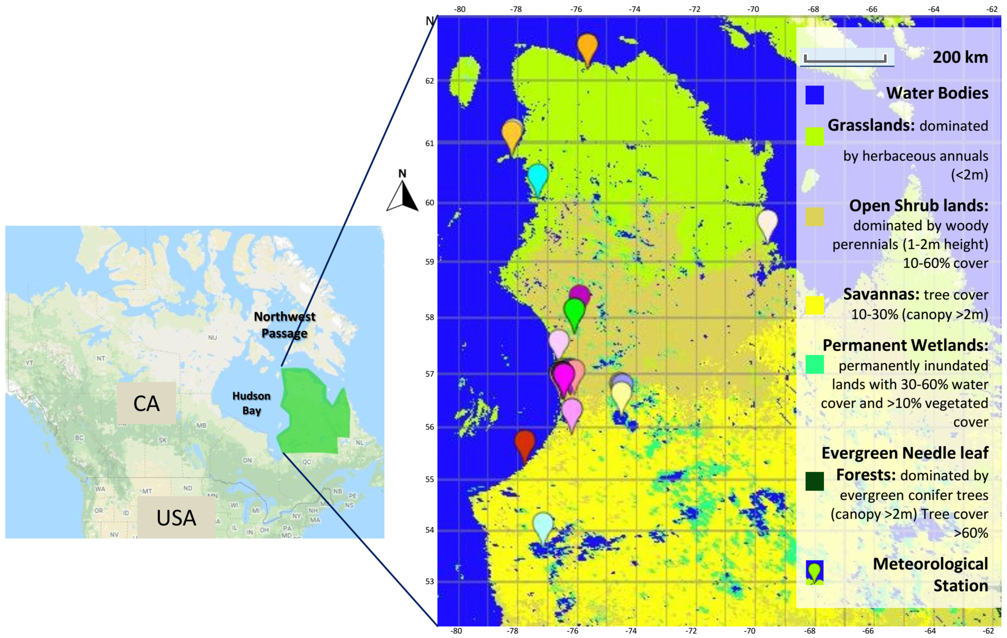
2.1. Study Area: Nunavik

The Nunavik region, Quebec, Canada was chosen as study area. This large region is very interesting for permafrost research since it shows high comprehensiveness and diversity by crossing several permafrost zones.

The climate of Québec varies highly depending on latitude, topography, and marine influence. The main types of climate in Nunavik are subarctic in the south and arctic in the north, both with long, very cold winters and short, cool summers with long hours of daylight. By crossing the borderline from the Arctic to the sub-Arctic, changes in vegetation cover and permafrost distribution can be observed, mainly reflected by the northern timberline and the substitution of discontinuous permafrost for continuous permafrost. In general, the climate in Nunavik can be characterized by low annual solar radiation, low temperature, low air humidity, and little precipitation [33]. Under the background of global climate change, the climate in Nunavik is also transforming. Slight cooling was measured from 1950 until the 1990s. According to Allard et al. (2007) [34], as of 1995, temperatures rose above the long-term average, and they have remained at elevated levels since the early 2000s [33].

In Quebec, permafrost extends from the sporadic discontinuous zone to the continuous zone (Figure 1). With general climate warming, ground temperature warming has occurred since the early 1990s with an increasing warming rate [35]. Over time, this has resulted in a warmer vertical temperature profile in the permafrost and a greater depth of summer thaw [36].

This region has attracted much research focused on permafrost studies, coastal geology, and geomorphological characterization [38,39,40,41,42,43,44,45]. Research by the CEN (Centre d’Études Nordiques) has been conducted here since 1980.

The concrete test sites were scattered over the large Nunavik region and were carefully selected with consideration of the data availability and computation efficiency. The variability over the region of interest was retained as much as possible.

2.2. SAR Sentinel-1

The Sentinel-1 (S1) mission is designed as a two-satellite (S1A and S1B) constellation. Since the launch of Sentinel-1A in April 2014, the Sentinel-1 mission continues to provide an all-weather, day-and-night supply of imagery of the Earth’s surface from a dual-polarization C-band synthetic aperture radar (SAR) instrument. The S1 data show a large advantage by providing free and open-access SAR data at high spatial and temporal resolutions with good stability.

For each study site, an individual S1 timeseries was built from images acquired from both the Sentinel-1A (S1A) and the Sentinel-1B (S1B) satellite constellations with the time limitation from the first available acquisition to August 2020. All images were level-1 ground range detected (GRD) products in ascending mode. The entirety of the database was acquired in the interferometric wide swath mode (IW) in both VV and VH polarization. In practical processing, the polarizations VV and VH were tested separately.

The S1 timeseries were all collected and created on the Google Earth Engine (GEE) platform, which is a planetary-scale platform for Earth science data and analysis powered by Google’s cloud infrastructure [46,47,48]. Every S1 scene on the GEE was preprocessed with the Sentinel-1 Toolbox using the following steps: thermal noise removal, radiometric calibration, and terrain correction using SRTM 30 or ASTER DEM for areas greater than 60° latitude, where SRTM is not available. The final terrain-corrected values were converted to decibels via log scaling (10 × log10(x)). In addition to the default preprocessing in GEE, several spatial filters were used to improve the data quality and evaluated in later chapters. The used spatial filters mainly included the basic moving window filter, in which the mean of the values of all pixels in the specified range was directly used as the value of the center pixel, and the gamma maximum a posteriori (MAP) speckle filter, which combines geometric and statistical properties to produce the values of the pixel and the average of neighboring pixels using moving windows.

2.3. In Situ Measurements

In this study, in situ temperatures acquired from the climate station network were used to derive the real-time FT state. Over the Nunavik region, 39 stations providing soil temperature measurements in a time period that overlapped the service time of the S1 Mission were found (Figure 2). Considering the possible sampling depth, only the measurements from the top 10 cm of the soil were taken into account.

The chosen stations were distributed mainly on the west side of Nunavik along the coastal area of Hudson Bay. These 39 stations were numbered according to their location from west to east and from north to south. The measurements from different soil depths within the top 10 cm were all kept and used separately, each as an individual layer. All available hourly data were compressed to daily average values. In the computation process, the temperature data were further selected by data quality and data size, and the surrounding environment was also a very important criterion. More details are shown in Section 3.1 and the table of station information in Appendix A.

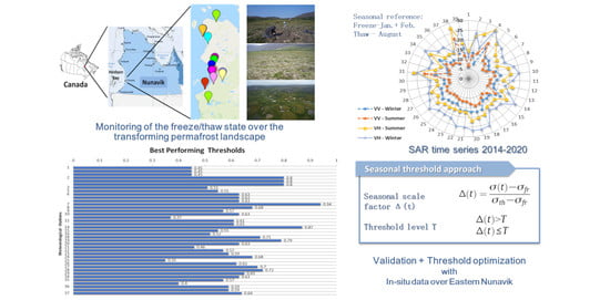
2.4. Seasonal Threshold Approach

To estimate the FT state, a seasonal threshold approach was used. This approach examines the timeseries progression of the remote sensing measurements relative to signatures acquired during seasonal reference frozen and thawed states. The key parameter in this approach is the seasonal scale factor Δ(t) (see Equation (1)), which can be calculated from σ(t), the measurement acquired at time t, for which an FT classification is pursued, and σ_fr and σ_th, the radar backscatter measurements corresponding to frozen and thawed reference states, respectively. After defining the seasonal scale factor Δ(t) at time t, this factor is then compared with a certain threshold to define the thawed and frozen landscape states (Equation (2)).

$$\Delta \left(t\right)=\frac{\sigma \left(t\right)-{\sigma }_{fr}}{{\sigma }_{th}-{\sigma }_{fr}}$$

(1)

$$\begin{gathered} \Delta \left(t\right)>T \\ \Delta \left(t\right)\le T \end{gathered}$$

(2)

To set the reference values of frozen and thawed states σ_fr and σ_th, two reference seasons of frozen (January + February) and thawed (August) states were defined. The frozen and thawed references were then computed for each grid cell of interest, individually, as an average of all existing S1 measurements acquired from their reference seasons during the period April 2014 to August 2020.

The FT algorithm is run on a grid cell-by-cell basis. To reduce the accidental bias of a single cell, the satellite observation data were preprocessed with a spatial filter (Section 2.2), and the test sites were carefully selected by considering the surrounding environment (Section 2.3). The output from Equation (2) is a dimensionless binary state variable that designates either frozen or thawed state for each cell of interest [16].

2.5. Validation and Threshold Optimization

To validate the estimated FT state, real-time temperature measurement data were used. A temperature threshold of 0 °C was set for the in situ data, which means that, when the measured temperature is higher than 0 °C, the soil state is set as thawed; otherwise, the soil state is defined as frozen. Every FT state that was estimated from the S1 image was then compared to the FT state that was determined on the basis of the temperature data, which were measured on the same date as the S1 acquisition. For S1 acquisition dates, where no exactly matching measurement is available, the nearest measurement within ±5 days (less than the shortest revisit time) was searched for usage.

To make the outputs from different locations more comparable, the calculated seasonal scale factors Δ(t) from Equation (1) were further normalized to the range of [0, 1]. Furthermore, an optimization step was included in the working process. Instead of fixing a threshold T (Equation (2)) at a certain value, the threshold was tested in a range of [0, 1] with a step of 0.01 during the estimation process. The accuracies of the tested timeseries were compared with each other to find the most effective threshold.

3. Results

This study aims not only to test whether the seasonal threshold approach can be used for retrieving the FT state in the Nunavik region but also to discuss the performance of Sentinel-1 SAR data in this method from different perspectives, including comparisons of the sensitivity of different polarizations, as well as the sensitivity at different surface soil depths. The analysis results are expected to pave the way for future works with more focus on FT state monitoring under diverse environments.

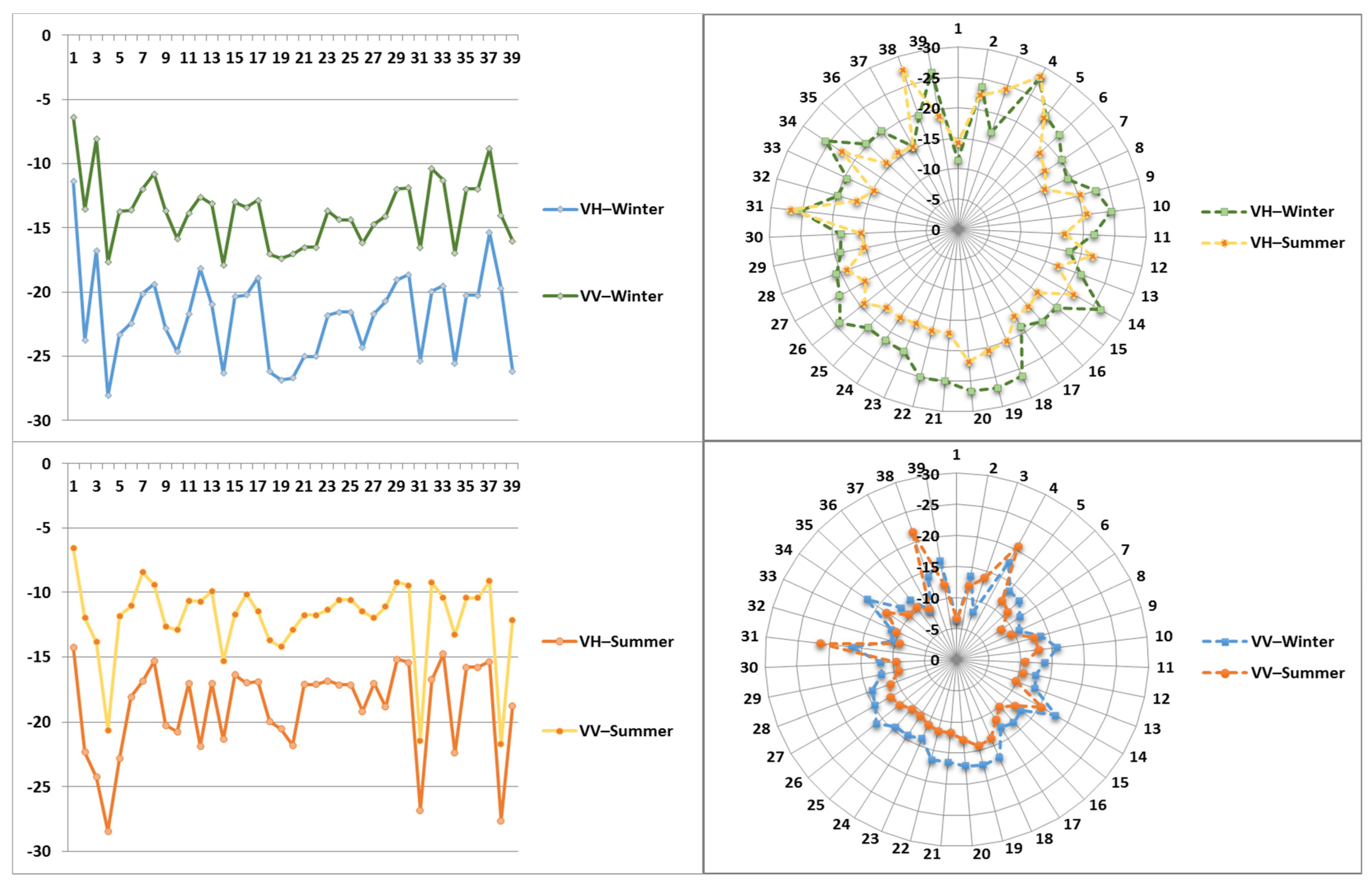
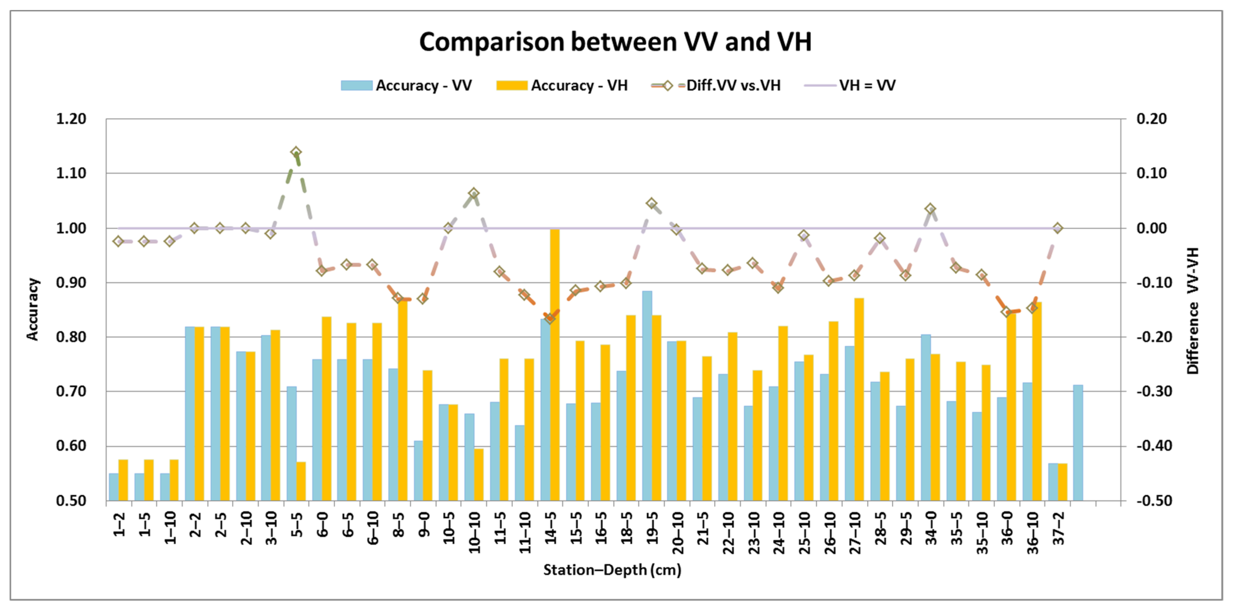
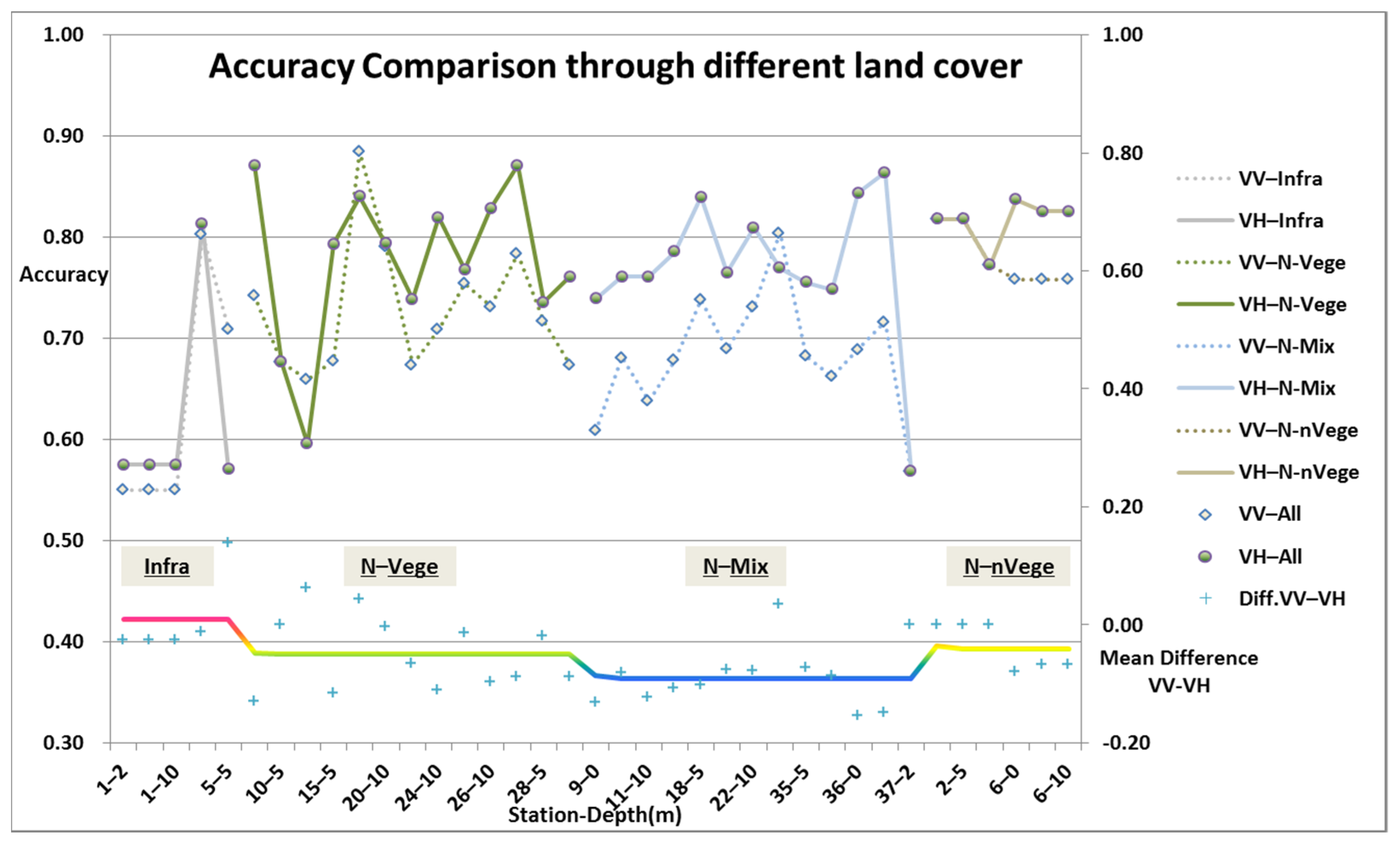
3.1. Backscatter Signal VH versus VV

As an essential component of the seasonal threshold approach, the backscatter signal from the Sentinel-1 data built the basis of the computation. In this study, the co-polarization vertical–vertical (VV) and the cross-polarization vertical–horizontal (VH) were used and tested separately. For each of the 39 possible validation test sites (

Table 1. Comparison of the results from datasets with and without values under −30 (Diff. > 0, blue; Diff. < 0, red).

Gamma3-Scale3
		Without < −30				With < −30
Station-Depth	Amount < −30	VV		VH		Diff. VV-VH	VH		Diff. VHwo-VHw
		Threshold	Accuracy	Threshold	Accuracy		Threshold	Accuracy
5–5	11	0.66	0.71	0.41	0.57	0.14	0.74	0.58	−0.01
6–0	5	0.62	0.76	0.64	0.84	−0.08	0.72	0.84	0.00
6–5	5	0.62	0.76	0.58	0.83	−0.07	0.72	0.84	−0.01
6–10	5	0.62	0.76	0.58	0.83	−0.07	0.72	0.84	−0.01
20–10	12	0.63	0.79	0.57	0.79	0.00	0.82	0.78	0.01
34–0	25	0.6	0.80	0.4	0.77	0.03	0.79	0.81	−0.05

), two SAR timeseries (VV and VH) containing 100 to over 200 data points from April 2014 to August 2020 were built.

The two timeseries from the same sites always had the same data size, whereas there was a significant difference between the values of the VV and VH timeseries. As shown in the left panel of Figure 3, the values of the VV timeseries from the chosen example sites were generally higher than the values of the VH timeseries. This phenomenon can be observed in all test sites, which means that, on a whole, the backscatter signal of the VH polarization was weaker than the signal of VV in the study area.

The overall trends of the two sets of timeseries were roughly similar, and seasonal fluctuations were fairly obvious. Compared with the more even distribution of VV data, there were more extreme values in VH data.

Considering the commonly used lower limit of −30, the quality of VH data was slightly worse since there were significantly more sites with substandard VH data, which were increasingly under −30. This difference can be observed at many sites. As shown in Figure 3, there were several points in each of the stations shown that were slightly lower than −30, while the whole timeseries was located in a value range clearly closer to −30 compared to their corresponding VV timeseries. This situation was particularly strong at the sites shown in the right panel of Figure 3. These stations were located in special or complex environments (P4 on a sandy plain with seashells; P31 close to Clearwater Lake; P38 on an island at the center of the Robert–Bourassa reservoir), for which the captured backscatter signal itself had a certain possibility of being negatively affected by the surrounding environment.

How this difference between VV and VH timeseries further affects the estimation result (Section 3.4) and whether some of these stations should be eliminated from the processing (Section 3.2) are tested and presented below.

3.2. Seasonal Reference Winter versus Summer

As one of the most important basic conditions in the algorithm, seasonal references have to be meaningful and representative. As shown in Figure 4, the references calculated from VV and VH for the 39 test sites shared almost the same curve for the same season, while the VH references were lower than the VV references overall, which also continues to confirm the observation in the previous section.

By comparing the references of summer (August) and winter (January + February), obvious seasonal differences can be observed in both polarizations. At most sites, the value of the summer reference was higher than that of the winter reference. There were also some counterexamples, mainly on the sites with controversial data quality mentioned in the previous site. In comparison, there were more sites from VH polarization that did not meet expectations than from VV polarization.

Considering the original quality and the performance of the timeseries data after preliminary calculations, some sites were carefully excluded in subsequent tests. The most relevant problem, leading to exclusion, was the limited data amount, at sites such as stations 12, 33, and 38, as well as the 10 cm layer of station 8. Here, the overlap between the in situ measured data and SAR data was too small to support the testing process. There were also arbitrary issues, such as the location pointed to by the coordinates of site 4 (in the water), which was inconsistent with the site description (on a sandy plain with seashells). Although these sites were not used for this work, they are still very valuable data in the Nunavik area; thus, they were kept in the summary of data to provide information for future work.

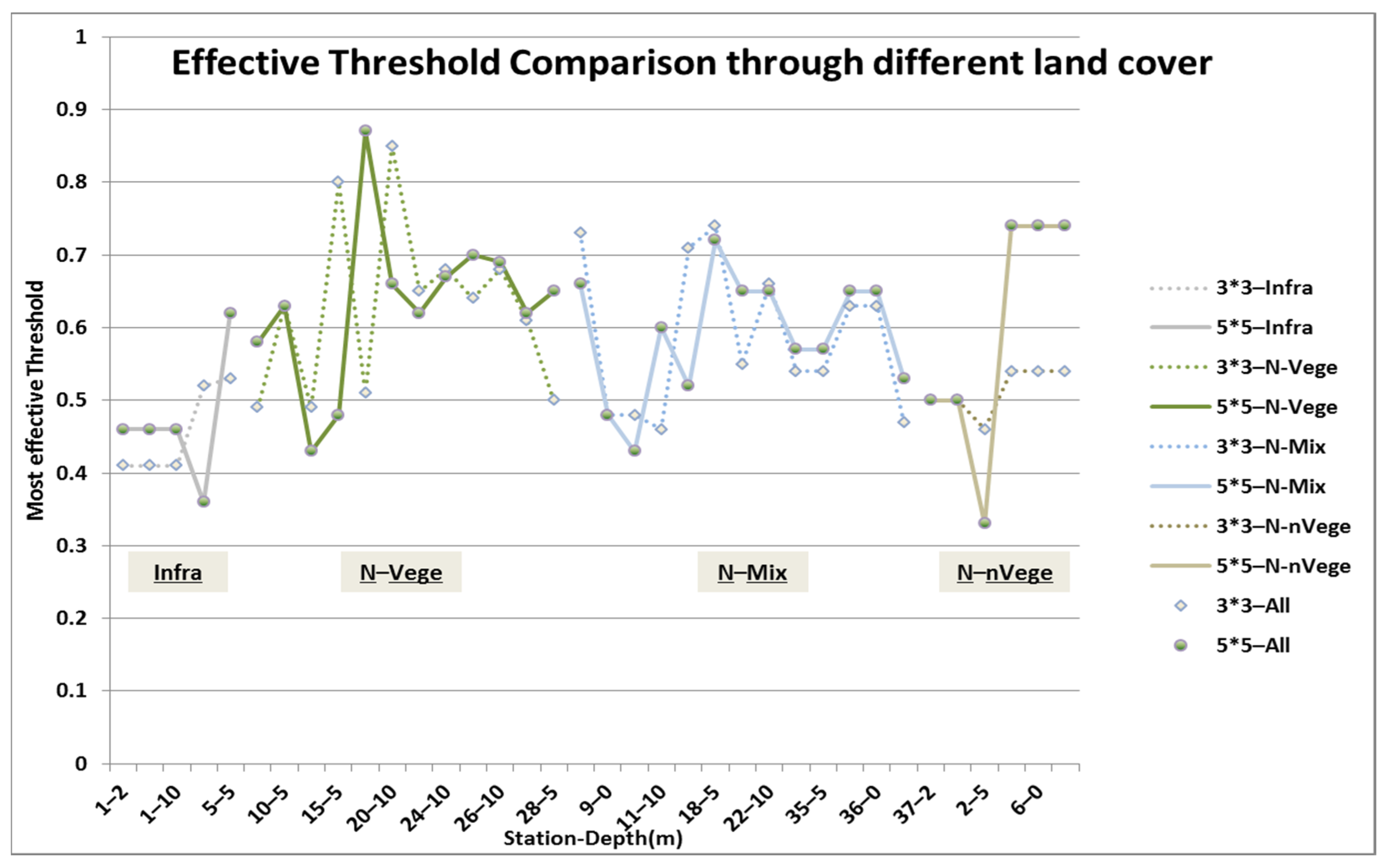
3.3. Threshold Distribution through All Selected Stations

As a result of the validation process with the 100-step threshold test, the accuracy distribution of each test site that varied with the changing thresholds was obtained. The threshold for each soil depth at each site to reach the highest accuracy is summarized in Figure 5. The accuracy of the sites had different forms of distribution, and there was not always a single threshold where the highest accuracy could be reached. This selection below is based on the statistics of the five thresholds that bring the top five accuracies of each depth of each site, and it shows the best-performing threshold or a representative of the best-performing thresholds.

As expected from the hypothesis, Figure 5 shows that the most effective threshold did not always fall within a fixed range. Many of the most effective thresholds were distributed between 0.55 and 0.65, which fits the commonly used range to a certain extent. However, in actual observations of each site, the fluctuation of the accuracy with the change in threshold was not the same. Meanwhile, there were also a non-negligible number of sites, which reached their optimal accuracy with a threshold that fell in other ranges. This could confirm the hypothesis that the reasonable adjustment of the threshold can help to improve accuracy, and test sites in different environments will respond differently to the threshold.

Within the same test site, the results from different depths shared almost the same distribution. For example, the 2 cm, 5 cm, and 10 cm layers of site 1 all reached their highest accuracy by setting the threshold as 0.45; the 2 cm, 5 cm, and 10 cm layers of site 2 reached their highest accuracy by setting the threshold as 0.8; the 0 cm, 5 cm, and 10 cm layers of site 6 reached their highest accuracy by setting the threshold as 0.63; the 5 cm and 10 cm layers of site 11 reached their highest accuracy by setting the threshold as 0.61; the 0 cm and 10 cm layers of site 36 reached their highest accuracy by setting the threshold as 0.59. Not only the best-performing threshold but also the overall change trend of the accuracy following the stepwise change in threshold was almost always the same between different testing depths from the same test site. This phenomenon indicates that the surficial 10 cm of soil reacts similarly in this approach without a significant difference in sensitivity to the thresholds.

This section mainly presents the analysis of the input data and the staged results in the calculation process. How well the seasonal threshold algorithm performs over the test sites, in other words, the exact accuracy, is shown in the next section.

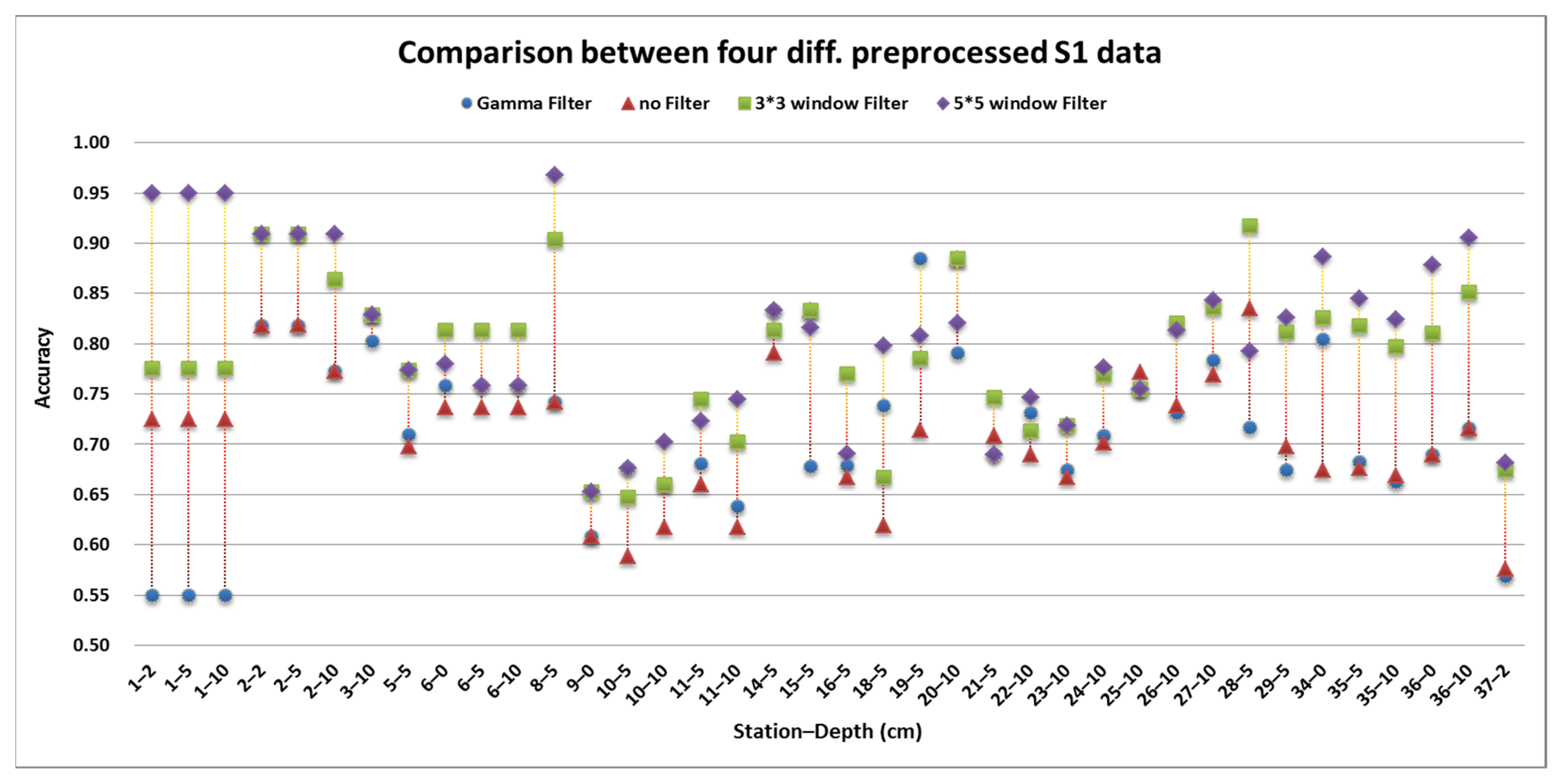
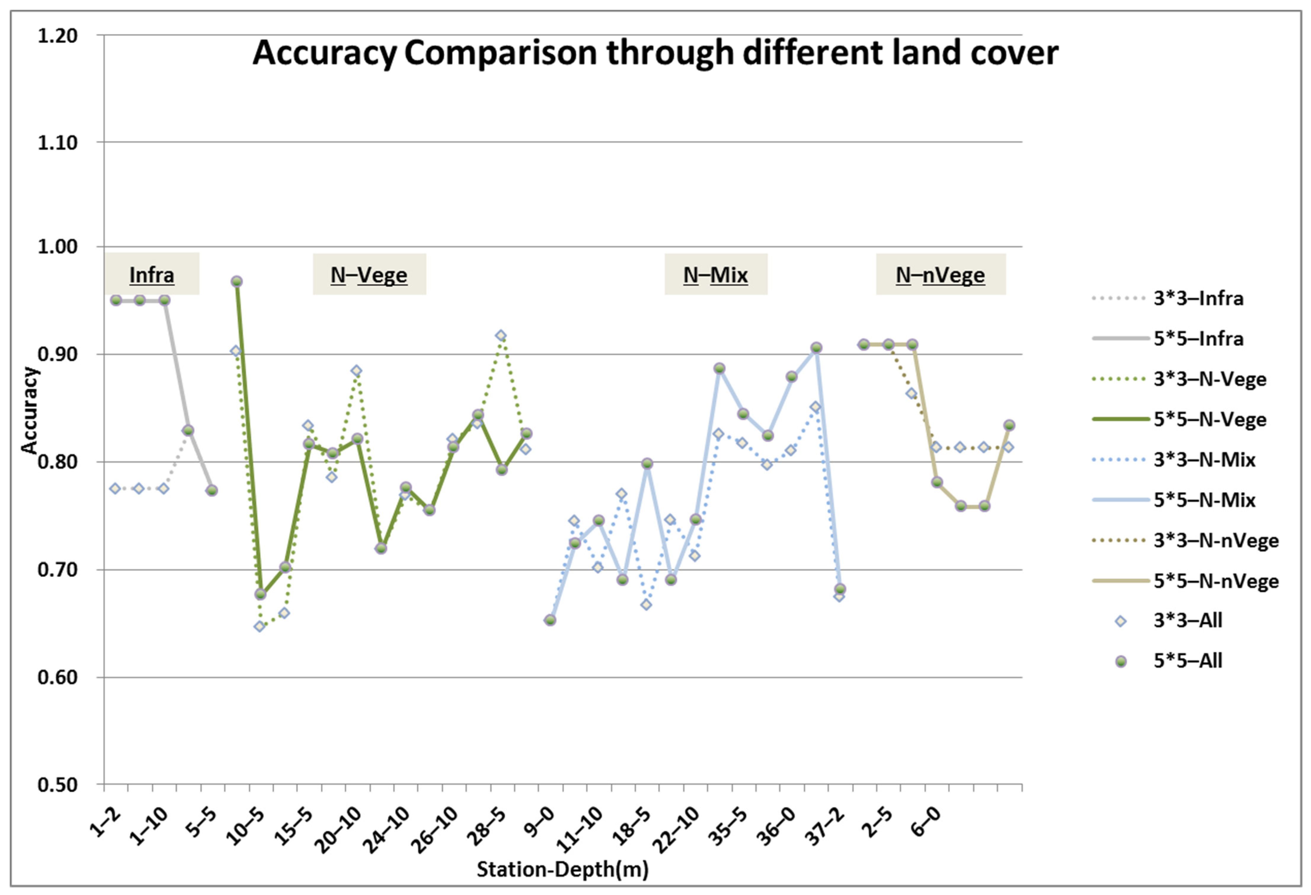
3.4. Accuracy and Analysis

This section mainly focuses on the comparison of the results from four test rounds. These four rounds differ by the settings of preprocessing of the Sentinel-1 data, i.e., the original backscatter signals without any spatial filter, the backscatter signals with a simple 3 × 3 window filter, the backscatter signals with a simple 5 × 5 window filter, and the backscatter signals with a 3 × 3 gamma filter. To reduce the repeatability, the comparison between the four rounds of tests focused only on the VV timeseries. The differences between the experimental results based on VV and VH data are presented under the setting with a gamma filter.

As shown in Figure 6, overall, relatively good results were achieved. On most tested layers, accuracy higher than 70% was achieved; the accuracy of the best-performing sites was higher than 90%. All the layers from the test round with a 3 × 3 window filter (green) had accuracies higher than 65%, except one with 64.7%, and the average accuracy reached 78.9%. The test round with a 5 × 5 window filter (purple) showed similarly good results, with the lowest accuracy of 65.2% and an even higher mean accuracy of 80.8%. The accuracy from the other two test rounds was overall lower, both with an average of approximately 71%, while there were very few layers with accuracies lower than 60%. The standard deviations of all four test rounds were not higher than 0.1; the lowest one was 0.072 from the test round with a 3 × 3 window filter, and the highest one was nearly 0.085 from the test round with a 5 × 5 window filter.

The different layers of the same sites again showed high similarity, which means that their highest accuracy was reached not only by setting the same threshold but also was very close or even the same value. In contrast, between different sites, the accuracy results were quite different. The ups and downs between the stations were relatively consistent in the three rounds of testing; in particular, the curves of the test rounds with the gamma filter and without the filter almost overlapped in multiple segments. This shows that the differences brought by different spatial filtering were relatively systematic adjustments. On the whole, the two window filters were most effective for this area, while each of them had better- and worse-performing sites, and the improvement effect brought by the gamma filter was less than expected.

Under the same filtering setting (gamma), there was also a difference in the sensibility between VV and VH polarization to be observed. Contrary to the observation in the previous section that the backscatter signals from VH polarization were generally weaker than those from VV, the accuracy achieved using VH data was almost always better than that achieved using VV data. As shown in Figure 7, there were a total of four layers where a higher accuracy was achieved in VV. There was no obvious commonality between these four layers, which may help to determine a common trigger for better performance of VV data. The accuracy difference of VV exceeding VH (green) was mainly within 10%, while the opposite difference (VH-VH, red) was approximately 10%, but no more than 20%. In general, VH data were not affected by a weaker signal and showed good usability in this approach. To further verify this statement, several test sites with remarkable but acceptable numbers of data points that were lower than −30 were chosen for testing. The test compared the accuracy of retaining and excluding data less than −30, and the results are summarized in Table 1. No significant differences were observed; in most layers, the result of not removing the too small value was even better than the result of removal. This shows that, in the range of the approach of this study, the lower VH value did not bring the expected adverse effects. At least when the number and range of values lower than −30 in the VH timeseries were controlled to a certain extent, there could be a certain degree of tolerance for usage of values lower than −30. Generally, for this study, VH polarization data can be considered a reliable or even better option than VV polarization data.

4. Discussion

4.1. Accuracy Aspect

In the previous section, it was shown that all rounds of testing showed good accuracy overall and there were differences between sites and between data from different preprocessing methods. To better understand these differences, we included statistics on the types and heterogeneity of land cover around the sites in our analysis.

The land cover around the test sites is classified into the following four categories according to the original site description and satellite data observations: one infrastructure-dominated category (Infra) and three natural environment-dominated categories: pure vegetation covered area (N-Vege), mixed environment (N-Mix), and area barely covered by vegetation (N-nVege).

The heterogeneity around the test sites was calculated on the basis of cloudless Sentinel-2 data in the summer of 2020. For each test site, the heterogeneity was calculated twice using two different buffers, with a radius of 17 m and a radius of 25 m, corresponding to the test rounds with a 3 × 3 window filter and a 5 × 5 window filter, respectively. For each test site, four values of heterogeneity were calculated, three based on three original bands of Sentinel-2 data (B2 blue, B3 green, and B4 red) and one based on NDVI data estimated using the red and NIR bands.

Considering that the results from the 5 × 5 window filter were obviously better than those of gamma- and non-filtering and were close to the results from the 3 × 3 window filter, while each had better- and worse-performing sites, the impact of heterogeneity on the accuracy is discussed by comparing the results from the 5 × 5 and 3 × 3 window filters.

By comparing the multiband heterogeneity of all test sites, a different level of correlation was found between the heterogeneity of the surrounding environment of the sites and the accuracy of the estimation. As shown in Figure 8, in most cases, the accuracy fluctuated in the opposite direction with the change in heterogeneity. Sites with large heterogeneity had relatively low accuracy. Conversely, sites with small heterogeneity had relatively high accuracy. Statistically, the overall correlation was not significant due to the different magnitude of the heterogeneity of the sites. When the land-cover information was taken into account, high correlation was found at the relatively bare sites, which were not dominated by vegetation (N-nVege and Infra), especially when a larger buffer was used.

When we further compared the performance of using two different buffers, we can see that, generally, the sites where the spatial heterogeneity was higher in the 5 × 5 buffer than in the 3 × 3 buffer tended to show better accuracy with the 3 × 3 window filtering process; conversely, when the heterogeneity around the station could be reduced by enlarging the buffer from 3 × 3 to 5 × 5, better accuracy was then reached with the 5 × 5 window filtering process. Additionally, a smaller spatial heterogeneity typically led to a smaller difference between the results from both filters.

Generally, the results of point-based testing reflect that the accuracy of the estimation was relatively affected by the heterogeneity of the surrounding environment. More homogeneous surroundings, which usually resulted in greater matching of the available signal to the exact land cover on the test site, enabled better accuracy. The spatial filter in the preprocessing, therefore, played an important role. For highly heterogeneous sites, a filter with a larger buffer could help to alleviate the influence of redundant signals, whereas using a coarser filter would also bring a greater risk of deviating from the original site environment. Therefore, in the use of the Sentinel-1 data, it is an important step to choose a suitable spatial filter that can effectively improve the quality of the data for extracting useful environmental information.

Furthermore, the results of the two polarizations VV and VH showed no obvious difference in response to heterogeneity. We sorted and counted the heterogeneity of the RGB and NDVI bands for sites with significantly better accuracy in VH than VV and sites with significantly better accuracy in VV than VH. The heterogeneity values of these two types of sites were very scattered, which means that the FT state at sites with a certain degree of (high/low) heterogeneity was not always better estimated in a certain polarization. In general, there is no direct indication that the difference in performance between the two polarizations was directly affected by the heterogeneity of the environment around the site.

When observing the accuracy of each soil layer at each site according to the land-cover grouping, the fluctuation of accuracy did not have direct directivity either. By using the gamma 3 × 3 filter (Figure 9), the results of the Infra group were overall lower than the others, and the results of the N-nVege group were relatively high, but this phenomenon was not repeated in the results using a 5 × 5 window filter. In general, according to the available results alone, there was no support for drawing strong conclusions about whether the land-cover type used by the algorithm in this study could perform better and how the land cover contributes to the detection process.

By further comparing the results of VV and VH considering the land cover, it can be seen that the difference between the results of VV and VH varied with the land cover (Figure 10). The N-Mix group showed the largest differences (VV vs. VH) with a mean of −0.09, the N-Vege and N-nVege groups had similar average differences of −0.05 and −0.04, respectively, and the Infra group had the only average difference greater than zero (0.01). VH was expected to show superiority over VV, especially in areas with dense vegetation coverage. The result is not entirely in line with the expectation. One regrettable point is that, because the analysis was based on sparsely distributed sites over large regions with very diverse surrounding environments, it could not meet the finer divisions, and the land cover could only be roughly classified to ensure the sample size of each type.

4.2. Threshold Aspect

Additionally, the effective threshold, on which the highest accuracy of a test site was reached, was further compared with the land-cover types (Figure 11). Observing from the average value alone, there was a clear distinction between the various categories. When the standard deviation and intuitive data distribution were taken into consideration (

Table 2. Average and standard deviation of each land-cover cluster.

Landcover	Infra		N-Vege		N-Mix		N-nVege
Filter	W 3*3	W 5*5	W 3*3	W 5*5	W 3*3	W 5*5	W 3*3	W 5*5
Mean	0.46	0.47	0.63	0.63	0.59	0.59	0.53	0.61
StD.	0.06	0.08	0.11	0.11	0.10	0.08	0.03	0.16

), the difference within a single category was relatively large, and there was no fundamental difference between categories.

In the practical optimization process, the distribution of the accuracies corresponding to thresholds of each site showed different forms. In the value range of 0 to 1, some sites had a clear and unique optimal threshold, some sites had multiple well-performing thresholds, some sites had continuous effective thresholds, and some sites had relatively smooth fluctuations in accuracy with the threshold. This situation increases the difficulty of finding a common useful optimal threshold directly based on land-cover categories.

In general, optimizing the threshold helps to achieve significantly better accuracy. The attempt to explore the optimal threshold with consideration of land cover is not meaningless; however, to obtain more effective results, it is necessary to perform more comprehensive statistics with larger data sizes, where more land-cover information, especially vegetation information, should be included.

5. Conclusions

Throughout the study, the seasonal threshold approach can be adequately used on C-band Sentinel−1 data. There is still space for accuracy improvement, for example, by improving preprocessing, such as filter adjustment, and further improving algorithms, such as threshold optimization. As a next step, it will be interesting to extend the recent point-based experiment to a larger area. The experiences collected in this study can be further used for testing and improving the functionality of the algorithm at the regional scale and for further exploration and discussion of the contribution of related variables such as land cover in the FT transition process.

Compared with L-band passive data, C-band SAR data have weaknesses in penetration depth and temporal coverage, but they can fill in the gaps of existing L-band products in spatial resolution. For more specific regional research, especially in permafrost landscapes with ever-changing environments, which have increasingly drastic changes in today’s climate change environment, the appropriate use of C-band data can provide more possibilities for detection and monitoring.

References

1. Burgess, M.M.; Smith, S.L.; Brown, J.; Romanovsky, V.; Hinkel, K. Global Terrestrial Network for Permafrost (GTNet-P): Permafrost Monitoring Contributing to Global Climate Observations: Current Research Report 2000-E14; Geological Survey of Canada: Ottawa, ON, Canada, 2000. Available online: http://dsp-psd.pwgsc.gc.ca (accessed on 10 December 2021).
2. Brown, J.; Hinkel, K.M.; Nelson, F.E. The circumpolar active layer monitoring (CALM) program: Research designs and initial results. Polar Geogr. 2000, 24, 166–258. [Google Scholar] [CrossRef]
3. Nelson, F.E.; Shiklomanov, N.I.; Hinkel, K.M.; Christiansen, H.H. The circumpolar active layer monitoring (CALM) workshop and the CALM II program. Polar Geogr. 2004, 28, 253–266. [Google Scholar] [CrossRef]
4. Ding, Y.; Ye, B.; Liu, S. Large-scale hydrological monitoring of frozen soil on the Qinghai-Tibet Plateau. Chin. Sci. Bull. 2000, 45, 208–214. [Google Scholar] [CrossRef]
5. Wang, L.; Derksen, C.; Brown, R. Recent changes in pan-Arctic melt onset from satellite passive microwave measurements. Geophys. Res. Lett. 2013, 40, 522–528. [Google Scholar] [CrossRef]
6. Mortin, J.; Schrøder, T.; Walløe Hansen, A.; Holt, B.; McDonald, K.C. Mapping of seasonal freeze-thaw transitions across the pan-Arctic land and sea ice domains with satellite radar. J. Geophys. Res. 2012, 117, C08004. [Google Scholar] [CrossRef] [Green Version]
7. Bartsch, A.; Kidd, R.; Wagner, W.; Bartalis, Z. Temporal and spatial variability of the beginning and end of daily spring freeze/thaw cycles derived from scatterometer data. Remote Sens. Environ. 2007, 106, 360–374. [Google Scholar] [CrossRef]
8. Bateni, S.M.; Huang, C.; Margulis, S.; Podest, E.; McDonald, K. Feasibility of characterizing snowpack and the freeze–thaw state of underlying soil using multifrequency active/passive microwave data. IEEE Trans. Geosci. Remote Sens. 2013, 51, 4085–4102. [Google Scholar] [CrossRef]
9. Jin, R.; Zhang, T.J.; Li, X.; Yang, X.G.; Ran, Y.H. Mapping surface soil freeze-thaw cycles in China based on SMMR and SSM/I brightness temperatures from 1978 to 2008. Arct. Antarct. Alp. Res. 2015, 47, 213–229. [Google Scholar] [CrossRef] [Green Version]
10. Judge, J.; Galantowicz, J.F.; England, A.W.; Dahl, P. Freeze/thaw classification for prairie soils using SSM/I radiobrightnesses. In Proceedings of the IEEE International Symposium on Geoscience and Remote Sensing, Singapore, 3–8 August 1997; pp. 827–832. [Google Scholar] [CrossRef]
11. Zhang, T.J.; Armstrong, R.L. Soil freeze/thaw cycles over snow-free land detected by passive microwave remote sensing. Geophys. Res. Lett. 2001, 28, 763–766. [Google Scholar] [CrossRef]
12. Zuerndorfer, B.; England, A.W. Radiobrightness decision criteria for freeze/thaw boundaries. IEEE Trans. Geosci. Remote Sens. 1992, 30, 89–102. [Google Scholar] [CrossRef]
13. Zuerndorfer, B.W.; England, A.W.; Dobson, M.C.; Ulaby, F.T. Mapping freeze/thaw boundaries with SMMR data. Agric. For. Meteorol. 1990, 52, 199–225. [Google Scholar] [CrossRef] [Green Version]
14. Jin, R.; Li, X.; Che, T. A decision tree algorithm for surface soil freeze/thaw classification over China using SSM/I brightness temperature. Remote Sens. Environ. 2009, 113, 2651–2660. [Google Scholar] [CrossRef]
15. Han, M.L.; Yang, K.; Qin, J.; Jin, R.; Ma, Y.M.; Wen, J.; Chen, Y.Y.; Zhao, L.; Lazhu Tang, W.J. An algorithm based on the standard deviation of passive microwave brightness temperatures for monitoring soil surface freeze/thaw state on the Tibetan Plateau. IEEE Trans. Geosci. Remote Sens. 2015, 53, 2775–2783. [Google Scholar] [CrossRef]
16. Derksen, C.; Xu, X.L.; Dunbar, R.S.; Colliander, A.; Kim, Y.; Kimball, J.S.; Black, T.A.; Euskirchen, E.; Langlois, A.; Loranty, M.M. Retrieving landscape freeze/thaw state from Soil Moisture Active Passive (SMAP) radar and radiometer measurements. Remote Sens. Environ. 2017, 194, 48–62. [Google Scholar] [CrossRef]
17. Kim, Y.; Kimball, J.S.; Mcdonald, K.C.; Glassy, J. Developing a global data record of daily landscape freeze/thaw status using satellite passive microwave remote sensing. IEEE Trans. Geosci. Remote Sens. 2011, 49, 949–960. [Google Scholar] [CrossRef]
18. Rautiainen, K.; Lemmetyinen, J.; Aalto, T.; Tsuruta, A.; Kangasaho, V.; Ikonen, J.; Cohen, J.; Kontu, A.; Vehvildäinen, J.; Pulliainen, J. Smos retrievals of soil freezing and thawing and its applications. In Proceedings of the IEEE International Geoscience and Remote Sensing Symposium, Valencia, Spain, 22–27 July 2018; pp. 1463–1465. [Google Scholar] [CrossRef]
19. Roy, A.; Royer, A.; Derksen, C.; Brucker, L.; Langlois, A.; Mialon, A.; Kerr, Y.H. Evaluation of spaceborne L-band radiometer measurements for terrestrial freeze/ thaw retrievals in Canada. IEEE J. Sel. Top. Appl. Earth Obs. Remote Sens. 2015, 8, 4442–4459. [Google Scholar] [CrossRef]
20. Roy, A.; Toose, P.; Williamson, M.; Rowlandson, T.; Derksen, C.; Royer, A.; Berg, A.A.; Lemmetyinen, J.; Arnold, L. Response of L-band brightness temperatures to freeze/thaw and snow dynamics in a prairie environment from ground-based radiometer measurements. Remote Sens. Environ. 2017, 191, 67–80. [Google Scholar] [CrossRef]
21. Kim, Y.; Kimball, J.S.; Glassy, J.; Du, J.Y. An extended global earth system data record on daily landscape freeze-thaw status determined from satellite passive microwave remote sensing. Earth Syst. Sci. Data 2017, 9, 133–147. [Google Scholar] [CrossRef] [Green Version]
22. Kou, X.K.; Jiang, L.M.; Yan, S.; Wang, J.; Gao, L.Y. Research on the improvement of passive microwave freezing and thawing discriminant algorithms for complicated surface conditions. In Proceedings of the IEEE International Symposium on Geoscience and Remote Sensing, Valencia, Spain, 22–27 July 2018; pp. 7161–7164. [Google Scholar] [CrossRef]
23. Wang, P.K.; Zhao, T.J.; Shi, J.C.; Hu, T.X.; Roy, A.; Qiu, Y.B.; Lu, H. Parameterization of the freeze/thaw discriminant function algorithm using dense insitu observation network data. Int. J. Digit. Earth 2018, 12, 980–994. [Google Scholar] [CrossRef]
24. Zhao, T.J.; Zhang, L.X.; Jiang, L.M.; Zhao, S.J.; Chai, L.N.; Jin, R. A new soil freeze/thaw discriminant algorithm using AMSR-E passive microwave imagery. Hydrol. Process. 2011, 25, 1704–1716. [Google Scholar] [CrossRef]
25. Rautiainen, K.; Lemmetyinen, J.; Schwank, M.; Kontu, A.; Ménard, C.B.; Mätzler, C.; Drusch, M.; Wiesmann, A.; Ikonen, J.; Pulliainen, J. Detection of soil freezing from L-band passive microwave observations. Remote Sens. Environ. 2014, 147, 206–218. [Google Scholar] [CrossRef]
26. Rautiainen, K.; Parkkinen, T.; Lemmetyinen, J.; Schwank, M.; Wiesmann, A.; Ikonen, J.; Derksen, C.; Davydov, S.; Davydova, A.; Boike, J. SMOS prototype algorithm for detecting autumn soil freezing. Remote Sens. Environ. 2016, 180, 346–360. [Google Scholar] [CrossRef]
27. Kim, Y.; Kimball, J.S.; Xu, X.; Dunbar, R.S.; Colliander, A.; Derksen, C. Global assessment of the SMAP freeze/thaw data record and regional applications for detecting spring onset and frost events. Remote Sens. 2019, 11, 1317. [Google Scholar] [CrossRef] [Green Version]
28. Colliander, A.; Mcdonald, K.; Zimmermann, R.; Schroeder, R.; Kimball, J.S.; Njoku, E.G. Application of QuikSCAT backscatter to SMAP validation planning: Freeze/thaw state over ALECTRA sites in Alaska from 2000 to 2007. IEEE Trans. Geosci. Remote Sens. 2012, 50, 461–468. [Google Scholar] [CrossRef]
29. Davitt, A.; Schumann, G.; Forgotson, C.; McDonald, K.C. The utility of SMAP soil moisture and freeze-thaw datasets as precursors to spring-melt flood conditions: A case study in the Red River of the North Basin. IEEE J. Sel. Top. Appl. Earth Obs. Remote Sens. 2019, 12, 2848–2861. [Google Scholar] [CrossRef]
30. Lyu, H.B.; McColl, K.A.; Li, X.L.; Derksen, C.; Berg, A.; Black, T.A.; Euskirchen, E.; Loranty, M.; Pulliainen, J.; Rautiainen, K.; et al. Validation of the SMAP freeze/thaw product using categorical triple collocation. Remote Sens. Environ. 2018, 205, 329–337. [Google Scholar] [CrossRef]
31. Roy, A.; Toose, P.; Derksen, C.; Rowlandson, T.; Sonnentag, O. Spatial variability of L-band brightness temperature during freeze/thaw events over a prairie environment. Remote Sens. 2017, 9, 894. [Google Scholar] [CrossRef] [Green Version]
32. Wang, J.; Jiang, L.; Cui, H.; Wang, G.; Yang, J.; Liu, X.; Su, X. Evaluation and analysis of SMAP, AMSR2 and MEaSUREs freeze/thaw products in China. Remote Sens. Environ. 2020, 242, 111734. [Google Scholar] [CrossRef]
33. Kativik Regional Government (KRG). Parc national des Monts-Pyramides Project. statues report. In Productive Safety Management; Kativik Regional Government: Kativik, QC, Canada, 2011. [Google Scholar]
34. Allard, M.; Fortier, R.; Sarrazin, D.; Calmels, F.; Fortier, D.; Chaumont, D.; Savard, J.P.; Tarussov, A. L’impact du Rechauffement Climatique Sur Les Aeroports du Nunavik: Caracteristiques du Pergelisol et Caracterisation des Processus de Degradation Des Pistes; Ouranos: Quebec City, QC, Canada, 2007. [Google Scholar]
35. Romanovsky, V.E.; Smith, S.L.; Christiansen, H.H. Permafrost thermal state in the polar Northern Hemisphere during the international polar year 2007–2009: A synthesis. Permafr. Periglac. Processes 2010, 21, 106–116. [Google Scholar] [CrossRef] [Green Version]
36. Allard, M.; Lemay, M.; Barrette, C.; L’Hérault, E.; Sarrazin, D.; Bell, T.; Doré, G. Permafrost and climate change in Nunavik and Nunatsiavut: Importance for municipal and transportation infrastructures. In Nunavik and Nunatsiavut: From Science to Policy. An Integrated Regional Impact Study (IRIS) of Climate Change and Modernization; ArcticNet Inc.: Quebec City, QC, Canada, 2012; pp. 171–197. [Google Scholar]
37. Obu, J.; Westermann, S.; Bartsch, A.; Berdnikov, N.; Christiansen, H.H.; Dashtseren, A.; Delaloye, R.; Elberling, B.; Etzelmüller, B.; Kholodov, A.; et al. Northern Hemisphere permafrost map based on TTOP modelling for 2000–2016 at 1 km2 scale. Earth-Sci. Rev. 2019, 193, 299–316. [Google Scholar] [CrossRef]
38. Beck, I.; Ludwig, R.; Bernier, M.; Lévesque, E.; Boike, J. Assessing permafrost degradation and land cover changes (1986–2009) using remote sensing data over Umiujaq, sub-arctic Québec. Permafr. Periglac. Processes 2015, 26, 129–141. [Google Scholar] [CrossRef] [Green Version]
39. Wang, L.; Marzahn, P.; Bernier, M.; Ludwig, R. Mapping permafrost landscape features using object-based image classification of multi-temporal SAR images. ISPRS J. Photogramm. Remote Sens. 2008, 141, 10–29. [Google Scholar] [CrossRef]
40. Wang, L.; Marzahn, P.; Bernier, M.; Ludwig, R. Sentinel-1 InSAR measurements of deformation over discontinuous permafrost terrain, Northern Quebec, Canada. Remote Sens. Environ. 2020, 248, 111965. [Google Scholar] [CrossRef]
41. Pelletier, M.; Allard, M.; Levesque, E. Ecosystem changes across a gradient of permafrost degradation in subarctic Québec (Tasiapik Valley, Nunavik, Canada). Arct. Sci. 2018, 5, 1–26. [Google Scholar] [CrossRef] [Green Version]
42. Ropars, P.; Lévesque, E.; Boudreau, S. How do climate and topography influence the greening of the forest-tundra ecotone in northern Québec? A dendrochronological analysis of Betula glandulosa. J. Ecol. 2015, 103, 679–690. [Google Scholar] [CrossRef]
43. Calmels, F.; Allard, M.; Delisle, G. Development and decay of a lithalsa in Northern Quebec: A geomorphological history. Geomorphology 2008, 97, 287–299. [Google Scholar] [CrossRef]
44. Allard, M.; Seguin, M.K. The Holocene evolution of permafrost near the tree line, on the eastern coast of Hudson Bay (northern Quebec). Can. J. Earth Sci. 1987, 24, 2206–2222. [Google Scholar] [CrossRef]
45. Hachem, S.; Allard, M.; Duguay, C. Using the MODIS land surface temperature product for mapping permafrost: An application to Northern Quebec and Labrador, Canada. Permafr. Periglac. Processes 2009, 20, 407–416. [Google Scholar] [CrossRef]
46. Gorelick, N.; Hancher, M.; Dixon, M.; Ilyushchenko, S.; Thau, D.; Moore, R. Google Earth Engine: Planetary-scale geospatial analysis for everyone. Remote Sens. Environ. 2017, 202, 18–27. [Google Scholar] [CrossRef]
47. Kumar, L.; Mutanga, O. Google Earth Engine applications since inception: Usage, trends, and potential. Remote Sens. 2018, 10, 1509. [Google Scholar] [CrossRef] [Green Version]
48. Mutanga, O.; Kumar, L. Google earth engine applications. Remote Sens. 2019, 11, 591. [Google Scholar] [CrossRef] [Green Version]
Figure 1. GlobPermafrost zonation, permafrost extent after Brown et al. (1997) and difference between borehole and modelled MAGT for Canada and Alaska, yellow frame: the Québec–Labrador Peninsula [37].
Remotesensing 14 00802 g001
Figure 2. Nunavik map with all test sites (base map: MODIS land cover type yearly global 500 m; https://lpdaac.usgs.gov/products/mcd12q1v006/, accessed on 10 December 2021).
Remotesensing 14 00802 g002
Figure 3. Backscatter signal time series of chosen test sites, left: stations 2, 6, and 36; right: stations 4, 31, and 38; blue, VV polarization; green, VH polarization.
Remotesensing 14 00802 g003
Figure 4. Backscatter signal reference of all test sites, left: comparison of references of different polarizations in the same season (top: winter, bottom: summer), right: comparison of references of the same polarization in different seasons (top: VH, bottom: VV).
Remotesensing 14 00802 g004
Figure 5. Best-performing threshold at different test soil depths at each site (0 cm, green; 2 cm, blue; 5 cm, yellow; 10 cm, red).
Remotesensing 14 00802 g005
Figure 6. Accuracy comparison of results based on differently preprocessed data.
Remotesensing 14 00802 g006
Figure 7. Comparison of the results from the two different polarizations.
Remotesensing 14 00802 g007
Figure 8. Environmental heterogeneity at each site of RGB and NDVI signals.
Remotesensing 14 00802 g008
Figure 9. Accuracy of different test soil depths, based on datasets from two preprocessing methods, clustered by four land-cover categories.
Remotesensing 14 00802 g009
Figure 10. Accuracy of different test soil depths: comparison between two polarizations, clustered by four land cover categories.
Remotesensing 14 00802 g010
Figure 11. Best-performing threshold at different soil depths, clustered by four land-cover categories.
Remotesensing 14 00802 g011