Abstract
Remote sensing is an effective method of evaluating building damage after a large-scale natural disaster, such as an earthquake or a typhoon. In recent years, with the development of computer vision technology, deep learning algorithms have been used for damage assessment from aerial images. In April 2016, a series of earthquakes hit the Kyushu region, Japan, and caused severe damage in the Kumamoto and Oita Prefectures. Numerous buildings collapsed because of the strong and continuous shaking. In this study, a deep learning model called Mask R-CNN was modified to extract residential buildings and estimate their damage levels from post-event aerial images. Our Mask R-CNN model employs an improved feature pyramid network and online hard example mining. Furthermore, a non-maximum suppression algorithm across multiple classes was also applied to improve prediction. The aerial images captured on 29 April 2016 (two weeks after the main shock) in Mashiki Town, Kumamoto Prefecture, were used as the training and test sets. Compared with the field survey results, our model achieved approximately 95% accuracy for building extraction and over 92% accuracy for the detection of severely damaged buildings. The overall classification accuracy for the four damage classes was approximately 88%, demonstrating acceptable performance.
1. Introduction
Over the past several decades, large-scale natural disasters have occurred much more frequently. According to the United Nations Office, disasters affected 4.2 billion people and resulted in approximately 2.97 trillion USD in economic losses globally [1]. To minimize economic loss and initiate appropriate rescue and recovery activities, a quick and accurate damage assessment is vital. Although a field survey could provide more detailed information, it also requires tremendous manpower and time. Under such circumstances, remote sensing technology becomes an alternate way to collect damage information effectively. Remote sensing systems have various platforms (i.e., spaceborne, airborne, and ground-based) using optical, synthetic aperture radar (SAR), and laser imaging detection and ranging (LiDAR) images to assess damage caused by nature disasters [2,3,4,5]. For example, Haq et al. [3] estimated how the flood affected land cover types and the number of people by using Moderate Resolution Imaging Spectro-radiometer (MODIS) onboard TERRA and AQUA images. As for building damage detection, various properties in spectra, textures, edges, spatial relationships, structures, shapes, and shadows of damaged buildings in post-event images have been used for damage detection. The visual interpretation of the optical images is still the basic approach for damage assessment, and the automatic damage detection process relies on the feature extractions. Although it is hard to determine the exact damage grade of a building using only post-event remote sensing images, they are useful to assess the damage as emergency responses.
Matsuoka and Yamazaki [6] visually estimated the building damage caused by the Boumerdes earthquake using the post-event QuickBird imagery. They found that the pre-event image was more important for the detection of lower damage grades in visual interpretation. In addition to visual interpretation, edges and textures are also used for post-event building damage detections. Vu et al. [7] developed an algorithm to detect the buildings affected by the Bam earthquake using post-event IKONOS and QuickBird images. More than 80% of the severely damaged buildings were classified correctly compared with the results of visual inspection.
SAR images are also employed for damage assessment of buildings. Although there are some difficulties in interpreting SAR imagery because of its oblique viewing geometry, occlusion, and ambiguity, especially for urban areas, it still has some benefits in disaster damage assessment due to its superior resolution and weather-independent surveillance. Matsuoka and Yamazaki [8] detected the phase information of backscattering echoes from ground objects to distinguish slight to moderate damage levels from SAR images. They found the degree of coherence was a good index to distinguish slight to moderate damage levels.
Airborne LiDAR systems allow fast and extensive acquisition of precise height data which can be used for detecting some specific damage types (e.g., pancake collapses) that cannot be identified from 2D images. Unfortunately, it is not a common practice to obtain laser scanning data right after a disaster only for the purpose of building damage detection. Therefore, methods with post-event LiDAR data alone have rarely been studied. However, if we can somehow obtain the pre-event LiDAR images, they may be very helpful for the building’s damage detection. Hussain et al. [9] applied the pre-event LiDAR data based on elevation information with post-event VHR imagery to improve the capability of building damage detection in the Haiti earthquake in 2010. It showed that elevation derived from LiDAR provides an important aid in determining first-floor collapsed buildings by introducing the missing dimension in the remote sensing imagery.
With the accumulation of data in recent decades, machine learning has played an increasingly important role in the detection of damages from natural disasters. As a subset of AI, machine learning allows software applications to become more accurate at predicting outcomes without being explicitly programmed with that ability. Machine learning algorithms use statistics to find patterns in massive amounts of stored data, including numbers, words, images, etc. In machine learning, supervised learning is the most preferred method for damage detection problems, such as support vector machine (SVM), random forests (RF), etc. Combining these methods with remote sensing images, many researchers have produced an accurate analysis and prediction of natural disaster damage [10,11,12,13]. Dornaika et al. [14] proposed a generic framework by applying a covariance descriptor to a building detection problem. They also tested classification performance with K-nearest neighbor, partial least squares, and SVM methods for the automatic and accurate detection of buildings from aerial orthophotos. Furthermore, with this concept, Naito et al. [15] developed machine learning models based on bag-of-visual words and SVM to predict the various damage grades within Mashiki town after the Kumamoto earthquake. The overall accuracy of different damage level classifications is approximately 57%. They also developed a deep learning model to compare with the machine learning method.
Deep learning is a subfield of machine learning that employs algorithms called artificial neural networks (ANNs), which are inspired by the structure and function of the brain. ANNs have several advantages. One of the most recognized advantages is that they can automatically learn from observations within datasets. However, as the image size increases, the number of trainable parameters of the ANN dramatically increases and results in non-optimal performance.
To solve this problem, an improved version of ANNs called convolutional neural networks (CNNs) has been suggested. The convolutional layer capability of this structure makes it an outstanding model for image processing among various image recantation tasks [16,17,18,19,20,21]. Krizhevsky et al. [22] presented AlexNet with five convolutional layers and three fully connected layers. Although AlexNet displays a more accurate performance than classical ANNs, when the stock layer increases, some problems such as gradient explosion begin to show up. To keep the gradient stable when training deep neural networks, two major improvements were created: residual blocks (ResNet) and identity mapping [23,24]. Long et al. [25] presented a new evolution architecture called fully convolutional network (FCN), in which the fully connected layers are replaced with convolutional layers in a CNN. This method produces an output image with the same size of input data.
Several methods were developed based on these improvements. In 2014, Girshick et al. [26] proposed a famous method called region-based convolutional neural networks (R-CNN) for object detection tasks. They indicated that the previous detection methods with a sliding window over all image pixels were wasting resources. Instead of running sliding windows, a region-based CNN only selects and runs some windows to obtain region proposals. In the following year, the same research group presented an evolutionary version called fast region-based convolutional network (Fast R-CNN) [27]. Compared with the previous methods, Fast R-CNN can reduce many redundant calculations due to highly overlapping regions. It also combined the classifier and the bounding box regression into a single network, enabling end-to-end training and boosting processing speed. Ren et al. [28] upgraded the Fast R-CNN into Faster R-CNN by switching the proposed method into region proposal networks (RPNs) for the calculation of anchor boxes. RPN takes a picture of arbitrary size as input and outputs a batch of rectangular region nominations, each corresponding to a target score and location information. Faster R-CNNs became state-of-the-art in 2015 and have been widely used in various object detection tasks since then [29,30]. In the detection of damages from natural disasters, Faster R-CNN still promises satisfying accuracy. Shetty et al. [31] compared the accuracy of building extraction between the traditional SVM and Faster R-CNN by training the model with the WorldView-2 dataset. Faster R-CNN method improved accuracy by 10% over SVM method within 2000 epochs.
While Faster R-CNN shows great performance in object detection, which is one of the three major focus areas of deep learning, researchers have begun new challenges to address both object detection and semantic segmentation simultaneously. He et al. and Lin et al. [32,33] provided a breakthrough with an instance segmentation method called Mask R-CNN and a feature extractor named feature pyramid networks (FPNs). With those improvements, Mask R-CNN is widely used in object recognition. Ullo et al. [34] used the images of landslides taken by a drone as the dataset to predict and mask the extent of landslides on mountains and gain a high accuracy result in the detection and segmentation tasks. Stiller et al. [35] investigated the correct detection rate of buildings with different architectural styles using a Mask R-CNN model, and the precision and recall exceeded 85% and 78%, respectively.
In Japan, local governments issue disaster victim certificates when a natural disaster occurs. The damaged buildings would be classified into several levels based on field investigation. However, according to the situations of past disasters, it took much time and labor to issue the certificates when the affected area was quite large. In the event of the Kumamoto earthquake, a total of 203,882 disaster victim certificates were issued in Kumamoto Prefecture until 11 May 2017 [36]. However, the certificates issued successfully in the first month were less than 30% of the requests. The delay of the certificate issuance was a severe problem for the life recovery of victims.
An effective and objective discrimination procedure of buildings’ damage level would help to shorten the issuance time of the disaster victim certificates. By visual interpretation of the pre- and post-event remote sensing images, we can assess the damage to buildings. Remote sensing images also support the automated change detection approaches which include image enhancements and post-classification comparisons. However, those methods require a professional knowledge in remote sensing or image processing field and might cause a human error. On the other hand, as a member of the R-CNN family, Mask R-CNN provides highly accurate results as reported in the previous studies, especially in the task with semantic segmentations.
Due to the improvement of efficiency and reduction of human errors and labor, the authors adopted Mask R-CNN for the damage assessment of the 2016 Kumamoto earthquake. We modified the Mask R-CNN model and applied it to post-event aerial images. The proposed model could extract buildings automatically and classify them with respect to the damage levels. The prediction results were verified after the comparison with the damage report of the field survey.
2. Datasets and Methods
2.1. Outline of the 2016 Kumamoto Earthquake
According to the Cabinet Office of Japan, the 2016 Kumamoto earthquake was a series of earthquakes, including two events: a moment magnitude (Mw) 6.2 foreshock and a Mw 7.0 mainshock. The mainshock occurred at 01:25 JST on 16 April 2016. Earthquakes of greater than 6 on a seismic intensity scale occurred 7 times from 14 April, as reported by the Japan Meteorological Agency (JMA). The distribution of the seismic intensity for the main shock in the Kyushu region is shown in Figure 1 [37]. A total of 273 people were killed and 2809 people were injured because of this event. More than 180,000 people were evacuated from the affected region after the earthquake. Severe damage to buildings was observed in the Kumamoto Prefecture. A total of 8657 houses completely collapsed, and approximately 190,000 residential buildings partially collapsed. In addition, the water supply was disrupted in 450,000 houses, power outage occurred in 480,000 houses, and the gas supply was shut off in 110,000 houses. The transportation network, including roads, railways, and air routes, was also severely damaged [38].
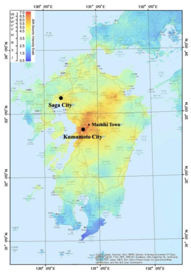
Figure 1.
Distribution of the JMA seismic intensity for the mainshock of the 2016 Kumamoto earthquake [37].
Mashiki Town, Kumamoto Prefecture, is one of the most affected areas. Ground motion with a JMA seismic intensity scale of 7 was observed twice in this area. In Mashiki Town, 28.2% of the buildings totally collapsed, 30.1% were severely damaged, 40.3% were partially damaged, and only 1.4% were undamaged [39].
2.2. Datasets
Five high-resolution post-event aerial images of Mashiki Town were used to create the dataset for building damage assessment. One aerial image consists of 14,430 × 9420 pixels. The resolution of the original aerial images is approximately 10 cm/pixel, and the bit depth is 24 bit. The aerial images were taken by the Geospatial Information Authority of Japan (GSI) using UltraCamX on 29 April 2016, two weeks after a series of earthquakes [40]. The five aerial images were mosaiced and covered the center of Mashiki Town, as shown in Figure 2. The most affected area was selected in the training and test sets. In Figure 2, the training area is covered with red, whereas the green color represents the test area.
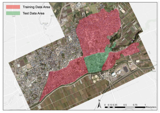
Figure 2.
Training and test sets generated from the five high-solution aerial images taken by GSI on 29 April 2016 [40].
Unlike the dataset of natural images, the viewpoint of remote sensing image datasets usually rests on the top, which makes the target objects appear relatively small. A single large-scale aerial image can contain over thousands of buildings. In this case, we cut the original image into 500 × 500 pixel square images by using the Photoshop slice function to obtain a total of 592 training images and 75 test images. The buildings located at the edge of the cut images would appear in two or more images. In this case, the key feature might be separated at different images, which leads to a decrease in detection accuracy. To solve this problem, we marked their complete shapes by shifting the cutting frame. Two examples are shown in Figure 3.
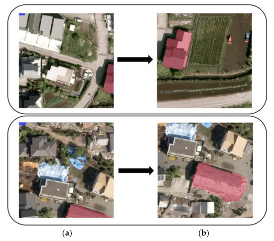
Figure 3.
Samples of buildings located at the edge, which are marked by the red masks. (a) Original cutting with incomplete shapes; (b) adjusted cropping frames with complete building shapes.
These cut images were labeled manually by the LabelMe tool into four damage categories [41]. The building damage categories were cited using the resources of the Architectural Institute of Japan (AIJ), from the report of the Ministry of Land, Infrastructure, Transport and Tourism (MLIT) [42]. The Kumamoto Earthquake Disaster Investigation Committee of the Kyushu Branch of the AIJ surveyed 2652 buildings, including the area around Mashiki Town’s Town Hall, the area around the strong motion observation station KiK-net Mashiki, and the southern area of Prefectural Road No. 28 up to the Akitsu River, where strong earthquakes had been recorded. The damage grades of the investigated buildings were classified based on the research of Okada and Takai [43,44]. The original damage grades of Okada and Takai were set from D0 up to D6. The MLIT report merged damage grades D5 and D6 into a “collapsed” label, including collapse and pancake collapse of the first floor, partial collapse, total crushing, and beam (roof) fracture. Damage grade D4 was transformed into the label “severe damage”. Damage grades D1 to D3 were merged into the label “slight damage”. The grade D0 was transformed as the label “no damage”. In this study, we used the same classification labels for the training and test sets. A detailed description of the damage classifications is shown in Table 1. Several samples of the labeled buildings are shown in Figure 4.

Table 1.
Definition of the damage grades used in this study [42,43,44].
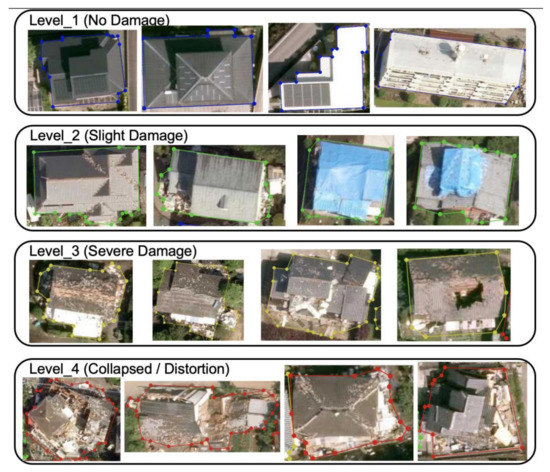
Figure 4.
Label examples of the buildings in levels 1 to 4.
2.3. Proposed Mask R-CNN Model
2.3.1. Mask R-CNN Architecture
Mask R-CNN is an object detection model based on Faster R-CNN developed by He et al. [32]. As shown in Figure 5, a mask prediction branch is added to Faster R-CNN. It also combines a feature pyramid network (FPN) with a residual network (ResNet) for feature extraction, to utilize multiscale information better. It replaces the Region of Interest Pooling (RoI Pooling) layer with the Region of Interest Align (RoI Align) layer. The bilinear interpolation method replaces the rounding method in the bounding box extraction to solve the problem of two quantization mismatches in the RoI pooling. This modification improves the accuracy of bounding box proposal.
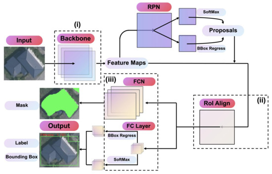
Figure 5.
Structure of the Mask R-CNN algorithm. (i) is the structure of Feature Pyramid Networks, (ii) is the structure of RoI, and (iii) is the original NMS structure.
The workflow of Mask R-CNN is as follows: (1) Mask R-CNN feeds the image to the residual network to extract features and generate multiscale feature maps; (2) side-joining is performed, and the feature maps at each stage are upsampled twice and tensor-summed with the adjacent underlying layers; (3) the feature maps are fed into RPN to generate candidate regions on the feature maps with different sizes that are input along with the feature maps to RoI Align to obtain the bounding boxes; and (4) the bounding boxes are classified and regressed, and a high-quality instance segmentation mask of the detected object is generated.
The feature extraction network of Mask R-CNN is formed by the union of an FPN and a ResNet, which is divided into two paths: bottom-up and top-down. The bottom-up path is the feedforward computation of the convolutional network, which is a residual module composed of different sizes of feature mappings of the residual network.
The RPN is an anchor-based structure that uses the feature map to calculate the position of the target object in the image. For k region proposals, the regression layer outputs 4 k coordinates, and the classification layer outputs 2 k scores to estimate the probability of object/nonobject for each proposal. RPN regresses each feature vector in the feature map and corrects the k anchors. The correction values of each anchor include coordinate values Δx, Δy, Δh, and Δw and classification values pf and pb. When the anchor correction is completed, a large number of bounding boxes are generated, and then only the more accurate bounding boxes will be filtered out by non-maximum suppression (NMS) based on the front and background scores of the bounding boxes to be passed into the subsequent RoI Align [26].
After acquiring the bounding boxes, the RoI pools the corresponding region into a fixed-size feature map according to the position coordinates of the bounding boxes for subsequent classification and envelope regression, as well as mask generation. RoI Align is a new regional feature aggregation method proposed in Mask-RCNN that directly crops the features at the corresponding positions of the candidate bounding box from the feature map and transforms the features into a uniform size by bilinear interpolation and pooling.
Finally, RoI Align extracts features from the region of interest and retains the exact location information of the pixels between the input and the output. The output from RoI Align forms two branches. The classification branch goes through a convolutional layer that has 7 × 7 convolutional kernels with 256 channels, then two fully connected layers with 1024-dimensional feature vectors, and finally completes the classification and the regression of the bounding box. The second mask branch goes through five 14 × 14 convolutional kernels with 256 channels, and then uses a 2 × 2 deconvolutional upsampling to generate a 28 × 28 feature map. Then, the feature map goes through a 1 × 1 convolutional kernel with a sigmoid loss function to obtain a 28 × 28 output, where every point in the output represents the front and background confidence of the bounding box in a certain category. Finally, a 0.5 confidence threshold is used to generate the object shape mask.
2.3.2. Model Modification
Although Mask R-CNN has a high-level capability in object detection, it still has some shortcomings when applied directly to damage detection from aerial images. Native Mask-RCNN has limitations of information loss in feature proposal network, and region proposal network (RPN) sometimes fails to localize either very big or small objects. Based on the above reasons, this paper proposes a Mask R-CNN-based model combined with the improved FPN presented by Liu et al. [45] and the online hard example mining (OHEM) proposed by Shrivastava [46] to improve the accuracy of objects of different sizes and solve the imbalance problems of positive and negative samples.
The structure of FPN has shown good performance in various applications; however, it has a side-joining step only for top-down paths, while a single size is selected from the paths of the final feature map input to the RPN layer. This design does not make full use of the feature information at each scale and may lose useful information on the remaining layers, resulting in a decrease in detection accuracy. To overcome this problem, Liu et al. proposed a modified feature pyramid network structure called the path aggregation network (PANet). The basic idea of this work is to shorten the information transmission path and use the precise location information of the lower-level features fully by adding bottom-up branches with reverse lateral connections to the feature pyramids [45]. As shown in Figure 6b, P2–P5 and N2–N5 are the feature mapping layers of FPN. The new bottom-up path is added by fusing the high-resolution feature map Ni with the coarser feature map Pi + 1 to generate a new feature map Ni + 1. The paper also suggested that both high- and low-level features are important for the feature map. The authors proposed pooling features from all levels and then fusing them to make predictions, which is called adaptive feature pooling and shown in Figure 6c. For each candidate region, the authors mapped it to different feature levels, as the gray regions in Figure 6b, and then use RoI Align to pool feature meshes from different levels and fuse the feature grids from different levels. The mask branch also used a fully connected fusion method by fusion the FPN and fully connected layer shown in Figure 6e. Better prediction results could be expected because of the merge of pixel-level prediction capability from FPN and the spatial location adaption capability from fully connected layer.
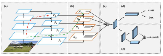
Figure 6.
Architecture of part (i) in Figure 5. (b) Bottom-up path augmentation was added to the original structure (a,c–e) [45].
When training the model, the RPN network randomly generates a large number of anchor boxes. Since the RPN provides the initial prediction and localization of the targets, it leads to the generation of too many background areas. If a single target object accounts for a small proportion of the image in a similar way to the remote sensing images used in this study, then it is easy to cause an imbalance between the number of positive and negative samples in the background and foreground, resulting in a difficult convergence of the network model and a poor detection performance. To solve the problem of imbalance between positive and negative samples during training, we use the online hard example mining (OHEM) algorithm presented by Shrivastava et al. in this framework to improve sample selection [46]. It does not require an artificial setting of the proportion of positive and negative samples, and neither does it degrade the network performance in real time. As mentioned in Section 2.2, the aerial photo was taken on 29 April, which the degree of cloudiness is under 10%. In this case, the main hard samples in this study are the nonresidential buildings as hard negative samples, such as secondary residences, garages, warehouses, etc. OHEM expands the original RoI network into two RoIs, one RoI with only forward propagation for calculating the loss and one RoI with normal forward-backward propagation, using the hard example as the input to calculate the loss and pass the gradient. The process of part (ii) of Figure 5 is shown in Figure 7 [46].
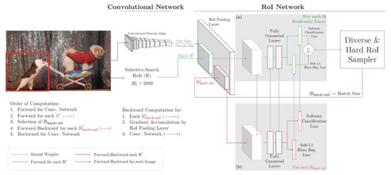
Figure 7.
Architecture of the proposed training algorithm specified as part (ii) in Figure 5: the proposed training algorithm: input image, selective search of RoIs, and computation of a conv feature map by the conv network. In (a), the read-only RoI network runs a forward pass on the feature map and all RoIs (shown by green arrows). Then, the Hard RoI module uses these RoI losses to select B examples. In (b), these hard examples are used to compute forward and backward passes by the RoI network (shown by red arrows) [46].
The greedy non-maximum suppression (NMS) algorithm is commonly used in object detection to solve the problem of overlapping prediction results, which was proposed by Girshick et al. [26] in 2014. However, the NMS algorithm addresses the case where there are multiple bounding boxes and masks overlapping in the same class. In this paper, because the appearance of buildings and their roof structures are similar, it is possible to have two different classes of bounding boxes for the same object. We modified the prediction process to fix this problem by simply applying the NMS algorithm again over the overlapping bounding boxes and masks. Only the results that have an intersection over union (IoU) with an over the threshold value will trigger this modification. The threshold value was defined by the data observations. The workflow of the modified NMS is shown in Figure 8.
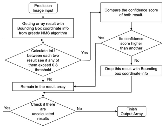
Figure 8.
Architecture of part (iii) in Figure 5: workflow (loop) of the modified NMS algorithm across multiple classes.
2.4. Details of Training and Evaluation Methods
The experimental environment is configured with an i7-4960X CPU, NVIDIA GeForce GTX 1080Ti GPU, CUDA: 11.2, Linux Ubuntu 18.04 LTS, with 23.4 GB memory. We used Python language to compile the code and used a PyTorch-based deep learning framework to test and train the relevant code. The original Mask R-CNN model was implemented with the mmdetection branch developed by open-mmlab [47]. The optimizer used in Mask R-CNN during training is stochastic gradient descent (SGD) with momentum. The details of the training parameters are shown in Table 2. Those parameters were optimized by several rounds of tests.
Table 2.
Details of the training parameters.
The Mask R-CNN model defines a multi-task loss on each sampled RoI as Equation (1) [32]
where stands for a classification loss used as a classical Binary Cross-Entropy loss, and the stands for bounding box regression loss used as a SmoothL1 loss [27]. The Binary Cross-Entropy loss was also used to evaluate . [32]. Equations mentioned above were shown in the Equations (2)–(4) [27,48]:
where is the distribution of the true values and is the distribution of the predicted values.
where , stands for the coordinate of the Ground Truth (GT) label, and , stands for the coordinate of the Predict Result (PR).
where x is the difference in values between the PR and GT.
To assess the performance of the proposed model, three sets of evaluation metrics were used. The first series of metrics consists of Precision, Recall, and Overall Accuracy (OAA), as defined in Equations (5)−(7) [49,50]. The definitions of True Positive (TP), True Negative (TN), False Positive (FP), and False Negative (FN) for multiclassification are shown in Table 3. Table 3 shows an example when the metrics are calculated for the label of Level_2.
Table 3.
An example of the definitions of TP, TN, FP, and FN for damage level_2.
The second metric is Intersection over Union (IoU). The IoU evaluates the overlap between the ground truth (GT) and predicted result (PR). In the object detection task, if the IoU value between the PR and GT is greater than a certain threshold value (normally set to 0.5), the model is considered to have correct outputs. IoU is defined as Jaccard index in Equation (8) [51]:
where J (A, B) stands for IoU. A is GT and B is PR.
The third series of metrics include average precision (AP) and mean average precision (mAP). AP is the area under a curve called the precision-recall curve (P-R curve, p (r)) for each class based on the recall and precision results. Its calculation is shown in Equation (9) [52], where mAP is the average of all APs.
The latest object detection works tend to use the COCO dataset to demonstrate the effectiveness of their models. For the COCO dataset, an interpolated AP calculation is used by sampling 100 points on the PR curve. Moreover, the threshold of IoU is taken in the range of 0.5–0.95 with intervals of 0.05, and average of AP values are calculated with these settings [53]. This average AP value will be taken as the final result.
3. Results
3.1. Experiment Results
Due to the narrow spacing between the buildings and unregular shapes, before training our modified model, we ran several tests on the original Mask R-CNN model to determine the best RPN parameters for this dataset. The results are shown in Table 4.
Table 4.
Comparison of the results using different RPN parameters in the original Mask R-CNN model.
Table 4 shows that the mAP of model-5 with the adapted RPN parameters is approximately 4% higher than that of the original model-1. Then, we experimented with several modified models based on the Mask R-CNN model-5. Several combinations of PANet and OHEM with different epochs are tested, for which results are shown in Table 5.
Table 5.
Comparison of the test results using modified models based on the Mask R-CNN model-5.
When we tested the parameters of RPN, we found that the current setting of 300 epochs tended to lead to overfitting and to cause low accuracy. Therefore, we decreased the epochs to 80, which gave us a direct mAP improvement of nearly 1%. We then tested the model with different strategies. When PANet and OHEM were applied independently, they both improved the results by approximately 2%. When they were both applied, the improvement reached 3–4%. Finally, we performed additional tests on model-9 with different numbers of epochs and chose 40 epochs as the final epoch value. The mAP of the bounding box was 0.365 and that of the segmentation was 0.373 in model-10. The curves of the training losses and accuracy in model-10 are shown in Figure 9. The training losses shown in Figure 9 include classifier loss (Classifier_loss), bounding box regression loss (BBOX_loss), mask branch loss (Mask_loss), and average loss (Avg_loss).
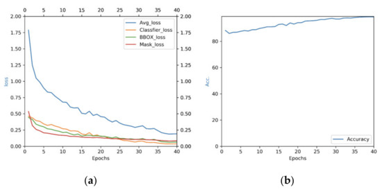
Figure 9.
Training curves of (a) losses and (b) accuracy associated with the best model (model-10).
We used the results of model-10 to make predictions on the data from the test set. In the test area, 95.1% of the buildings were identified successfully. The precision of building detection was 91.4%. The OAA of the building extraction was 87.3%. Even the severely damaged buildings (Level_3 and Level_4) could be extracted with 86.1% OAA. The precision and recall of building detection reached 92.0% and 94%, respectively. The misdetections were caused by delineations between two buildings or hidden shadows of other buildings. On the other hand, over detection was caused by buildings that were not investigated by the AIJ. However, our model detected those buildings and estimated their damage grades.
The classification precision of Level_1 exceeded 83%, and recall was 76%. The precision and recall of Level_2 were 72% and 88%, respectively. The precision of Level_3 was 83%, and recall was greater than 70%. For the total collapsed buildings in Level_4, the precision exceeded 93% and recall was approximately 85%. The OAA of the classification reached 82%. The confusion matrix for the test area is shown in Table 6, which showed acceptable results. Most of the damaged buildings were classified into the accurate class or its neighboring class. Two buildings in Level_2 were overestimated to Level_4, where one of them is shown in Figure 10(a1,b1). This Level_2 building was close to a Level_4 building, and our model detected them as one building with the label of Level_4. Eight collapsed buildings in Level_4 were underestimated to be Level_2. This type of error is mainly caused by the partial collapse or pancake collapse of the first floor, whereas the rooftop remained in good condition. An example is shown in Figure 10(a2,b2).
Table 6.
Confusion matrix of the damage classification for the buildings in the test area.
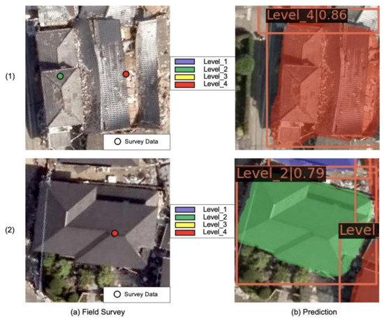
Figure 10.
Misclassification situations of the proposed model-10.
To evaluate the validity of PANet and OHEM, we also compared the building extraction accuracy and classification accuracy of model-10 with those of model-6. For model-6, the OAA of building extraction was 84.1%. As for the classification, the average precision of 4 classes is 74.9%; the average recall of 4 classes is 77.8%. On the other hand, model-10 performed 3.2% higher than model-6 with an 87.3% OAA of building extraction. The average precision and recall of model-10 are also 7% and 2% higher than those of model-6. The PANet and OHEM methods improved both classification and building extraction capability of the model.
Based on these results, we applied model-10 to the whole target area of Mashiki Town and obtained a prediction map of building damage, as shown in Figure 11. From the prediction map, we can see that most of the collapsed buildings (Level_4) were around the No. 28 Prefectural Road. More than half of the buildings were classified into Level_1 and Level_2, indicating no damage or less than moderate damage, respectively.
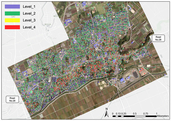
Figure 11.
Obtained prediction map of all the buildings in the target area using the proposed model-10.
3.2. Verification
To verify the accuracy of our prediction map, we compared it with the report of the AJI for the 2016 Kumamoto Earthquake. In the AIJ report, the ratios of collapsed buildings were summarized and calculated in 57-m grids. The grids were defined based on the Basic Grid Square, which was announced by the Administrative Management Agency of Japan [54]. One Basic Grid Square is divided into 20 sections in the east–west direction and 16 sections in the north–south direction. Thus, one grid in our study was approximately 57 m × 57 m.
The ratio of the number of collapsed buildings to that of all buildings in the grid was calculated. The grid map of the collapsed ratio is shown in Figure 12a. There were 414 grids in the target area of the field survey, which were classified into five classes according to the collapse rates. There were 262 grids in the class of 0%, 47 grids in the class of 0–25%, 53 grids in the class of 25–50%, 37 grids in the class of 50–75%, and 10 grids in the class of 75–100%. To verify our predication results, we calculated the ratio of Level_4 buildings in Figure 11 using the same grid scale, and it is shown in Figure 12b. There are 260 grids in the class of 0%, 45 grids in the class of 0–25%, 62 grids in the class of 25–50%, 36 grids in the class of 50–75%, and 11 grids in the class of 75–100%.

Figure 12.
Comparison of (a) the collapsed ratio in the report of the field survey [42] and (b) our prediction in a 57-m grid unit.
For each class of collapsed ratios, we obtained a decent result. The precision and recall for the collapsed ratio of 0% reached 99.2% and 98.9%, respectively. For the collapse ratio of 0–25%, the precision was 93.3%, and the recall was 89.4%. Additionally, the grids associated with the collapse ratio of 25–50% had 85.3% and 98.1% precision and recall, respectively. The precision and recall for a collapse ratio of 50–75% reached 100% and 88.5%, respectively. For the collapse ratio of 75–100%, the precision was 81.8%, and the recall was 90.0%. The OAA of all the classes of collapsed ratios reached approximately 96%. The confusion matrix is shown in Table 7. Most of the grids were classified either in the accurate class or neighboring classes. A single non-collapsed grid was mistakenly classified as 25–50%, and another grid with a collapse ratio of 75−100% was underestimated as 25–50%. These were both caused by the differing counts of buildings. While some houses in Japan have primary buildings, secondary buildings, and warehouses, the field survey from the AIJ only recorded damage to primary buildings. In addition, unoccupied houses were not counted in the report. This led to the difference between the prediction results and the true data.
Table 7.
Confusion matrix of grid prediction in the whole investigated area.
The aerial images of these two grids are shown in Figure 13. Only one building in Figure 13(a1) was investigated by the AIJ, and it was classified as Level 2, as successfully detected by our model. However, our model detected four other buildings, and two of them were classified as Level_4, as shown in Figure 13(b1). Thus, the collapse rate of this mesh was estimated as 25–50%. In Figure 13(a2), there are four buildings investigated by the AIJ, with three in Level 4 and one in Level_1. In our results shown in Figure 13(b2), seven buildings were detected, with two in Level_4, four in Level_2, and one in Level_1. The two collapsed buildings were misclassified since their damaged parts were difficult to identify from the aerial images. Thus, the collapse rate of this grid was misestimated as 25–50% instead of 75–100%.
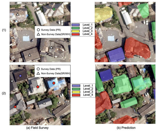
Figure 13.
Comparison of the buildings investigated by the AIJ (a) and those detected by our proposed model (b).
Since the prediction map in Figure 12 included the area used for the training set, we selected the grids containing only the test area, as shown in Figure 14. In a total of 37 grids reported by the field survey, there were 9 grids with the collapsed ratio of 0%, 7 grids with that of 0–25%, 9 grids with that of 25–50%, 9 grids with that of 50–75%, and 3 grids with that of 75–100%. For our prediction results, 9 grids were classified as the collapsed ratio of 0%, 7 grids as 0–25%, 12 grids as 25–50%, 7 grids as 50–75%, and 2 grids as 75–100%. The confusion matrix is shown in Table 8.
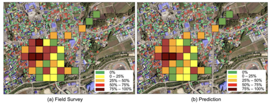
Figure 14.
Close-up of the comparison of the field survey and our prediction for the grids containing only the test area.
Table 8.
Confusion matrix of the grids in the test area.
The precision and recall for the grids with collapse ratios of 0% and 0–25% were 100%. The precision and recall for the grids with collapse ratios of 25–50% were 75%, and the recall remained at 100%. For the grids with collapse ratios of 50–75% and 75–100%, the precision for each reached 100%, and the recall reached 77.78% and 66.67%, respectively. The OAA of prediction for the test area reached 91%, which showed a high capability to detect severely damaged areas.
4. Discussion
To detect the buildings in aerial images and estimate their damage levels, we modified the Mask R-CNNs model and improved its performance on small object detection with similar features. A satisfactory accuracy suggests that the modification was successful and could obtain good predictions using the large-scale aerial images.
Firstly, we optimized the RPN hyperparameter through several cycles of experiments for a better adaptation of building spacing and building shapes. Two examples are shown in Figure 15. In Figure 15a, four neighboring buildings enclosed by the red line were close to each other with minimal space in between. In Figure 15b, the ratios of several buildings’ length and width were larger than 2, which is out of the range of the default RPN default parameter. With the anchor stride and the anchor ratios being expanded, the mAP of the detected buildings increased by 3–4% compared with the original parameter settings, and the prediction results of both detection and segmentation were better.
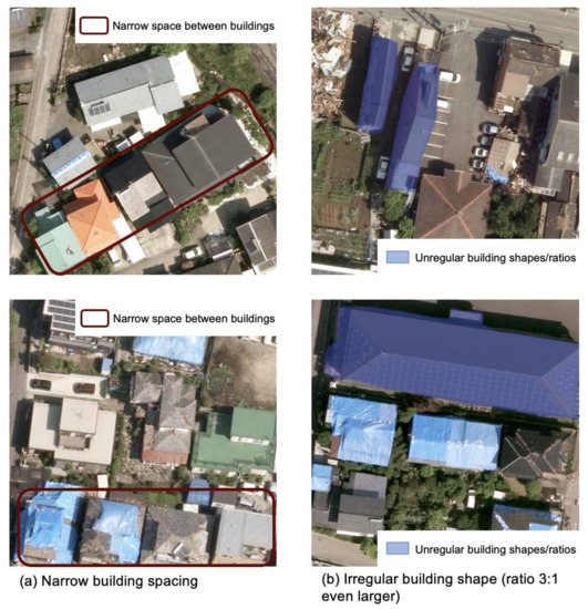
Figure 15.
Two examples of buildings that were difficult to detect by the original RPN parameters.
After hyperparameter optimization, three major modifications mentioned in Section 2.3.2 were conducted. In the dataset used in this paper, the features of the buildings damaged by the earthquake are quite similar. This makes it difficult to extract features using original FPN networks, especially in locating scattered rubble at the edges and subtle damage to the roofs. To overcome this problem, we applied PANet based on the best optimized model. In our experiments, the application of PANet alone led to an improvement in accuracy of approximately 2% for mAP.
When RPN generates anchor boxes on the feature map, due to the nature of aerial images, the building as the foreground target generates fewer anchors, while the rest of the contents as the background generates more anchors. Such an imbalance sampling of anchors will tip the scale toward negative anchor samples, and thus reduce the recall of the model and the classification OAA.OHEM embeds the hard example mining mechanism into the SGD algorithm, so that the model can automatically select suitable region proposals as either positive or negative examples during the training process based on the loss of region proposals. Additionally, the scores of RoI proposal prediction by the R-CNN subnetwork (b) in Figure 7 were used to determine the samples selected for each batch. In this way, the RoI proposal input to the R-CNN subnetwork (b) will always be the hard negative examples for which the current network performs worst, improving the efficiency of supervised learning. The mAP of the model increased 2% under the OHEM algorithm, and it increased 1% more when applied simultaneously with PANet.
The final modification is in NMS. We applied the model-10 to the test data, and the results are shown in Figure 16b. We noticed that the overlapping prediction bounding boxes occur in the plot of Figure 16(b1). The building in the lower left corner was detected and classified to be as the classes of level_3 and level_4 at the same time, while the bounding box of level_4 which overlapped at the top is not the optimal result. This is because the damaged buildings in adjacent categories have many similar features and are prone to have overlapping bounding boxes in different categories with lower confidence. The greedy NMS algorithm proposed by Girshick et al. [26] achieves a good result on a single object with only one class per image, but not good enough in crowded scenes or multi-class satiation [55]. Thus, we improved the NMS algorithm so that it can perform class filtering in the prediction task across classes and maintain the bounding boxes of the class with the highest confidence. The improved results are shown in Figure 16c. By applying these three modifications, the proposed model improved mAP by 3% both for the bounding box and the segmentation. Additionally, the OAA for the whole area was 96%, and that for the test area was 91%.
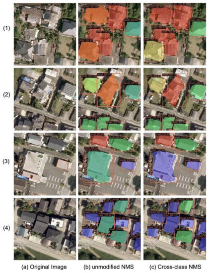
Figure 16.
Comparison of the results (a) without the NMS, (b) with default NMS, and (c) with those after applying the multiclass NMS approach without overlapping.
With the improvement mentioned above, we compared our results with previous studies for damage estimation of the buildings using the 2016 Kumamoto earthquake image. Liu et al. [56] achieved an OAA of approximately 46.8% in the classification of damaged buildings by using multitemporal PALSAR-2 data. Although SAR images can be obtained despite weather conditions, damage assessment from SAR images with high accuracy is still difficult. Naito et al. [15] developed both SVM and CNN models. For the SVM model, it performed 56.6% OAA for the damage classification; precision and recall rates also fluctuated between different categories. As for the CNN model, it performed an 88.4% OAA for the damage classification and average 80% precision and recall. However, both models are based on the evaluation indicators of personal visual interpretation, which might lead to a certain perceived error that may arise from human mistake. On the other hand, our model achieved the same level of OAA of 88.1% based on the verification of the report of the MLIT field survey. Compared with the verification using visual interpretation, the performance of our model is more objectively evaluated. In addition, our modified NMS approach gave a prediction map with an accuracy of 91% OAA for the collapsed ratio, which would be potentially useful for the emergency response after an earthquake.
Based on the above comparison, our proposed model can be applied for damage assessment after an actual earthquake. Buildings can be detected with an accuracy of approximately 90%, and their damage levels are classified properly with an accuracy of approximately 80%. Our model is helpful to reveal the most affected areas and accelerate the rescue process.
On the other hand, the accuracy of our model depends on the information in the dataset. Thus, when the resolution of images is not high enough to identify the debris surrounding the collapsed buildings, the prediction accuracy might decrease. The acquisition time of post-event images is also an important element in the actual damage detection. When the post-event images are obtained too late after the clear-up, the prediction accuracy for the severe damage including level_3 and level_4 might also decrease.
There are two major limitations for the proposed model. First, the damage to walls and the collapse of the first floor could not be detected by our model since aerial ortho-images were used in this study. That leads to an uncontrollable decrease in the accuracy of our results compared with the results of field survey. Several misclassifications are shown in Figure 10. The oblique aerial images may be useful to solve this problem. The second limitation is the lack of data. Our model was trained and tested using only the dataset from the 2016 Kumamoto earthquake. It might be difficult to apply to other events directly, but it can be used as the base model for transfer learning to other earthquake events.
5. Conclusions
In this paper, we aim to develop a faster means to extract damaged buildings and estimate their damage levels using high resolution aerial images taken after the 2016 Kumamoto earthquake. We modified the original Mask R-CNN model by adding PANet, OHEM, and the modified NMS, which improved the mAP of the model from 29% to 37% and enhanced the capability of detecting small objects with similar features. By training and testing the aerial images, 95.1% of the buildings were detected successfully, and the overall accuracy of the damage classification was 88%.
The best model was applied to the entire target area of Mashiki Town, Kumamoto Prefecture, Japan, and a prediction map of building damage was obtained. The prediction results were verified by comparison with the field survey report of the MLIT. The ratios of the collapsed buildings in the 57-m grids were calculated. The accuracy in the test area was approximately 91%. The results support that the proposed model is a viable method of quickly extracting damaged buildings due to earthquakes from post-event aerial images. For further research, we will focus on different regions or different earthquakes by using transfer learning to create a general solution for the damage detection after natural disasters.
Author Contributions
Y.Z.: conceived the work, processed the data, and wrote the paper. W.L. and Y.M. supervised the data processing and revised the manuscript. All authors have read and agreed to the published version of the manuscript.
Funding
This research was supported by “the Tokyo Metropolitan Resilience Project” of the Ministry of Education, Culture, Sports, Science, and Technology (MEXT) of the Japanese Government, the National Research Institute for Earth Science and Disaster Resilience (NIED), and Niigata University.
Institutional Review Board Statement
Not applicable.
Informed Consent Statement
Not applicable.
Data Availability Statement
No new data were created in this study. Data sharing is not applicable to this article.
Acknowledgments
The high-resolution aerial images used in this study are the property of the Geospatial Information Authority of Japan. The field survey data of building damage were investigated and owned by the AIJ.
Conflicts of Interest
The authors declare no conflict of interest.
References
- The Human Cost of Disasters: An Overview of the Last 20 Years (2000–2019). Available online: https://www.undrr.org/publication/human-cost-disasters-overview-last-20-years-2000-2019 (accessed on 27 October 2021).
- Plank, S. Rapid damage assessment by means of multi-temporal SAR—A comprehensive review and outlook to Sentinel-1. Remote Sens. 2014, 6, 4870–4906. [Google Scholar] [CrossRef]
- Haq, M.; Akhtar, M.; Muhammad, S.; Paras, S.; Rahmatullah, J. Techniques of remote sensing and GIS for flood monitoring and damage assessment: A case study of Sindh Province, Pakistan. Egypt. J. Remote Sens. Space Sci. 2012, 15, 135–141. [Google Scholar] [CrossRef]
- Wang, W.; Qu, J.J.; Hao, X.; Liu, Y.; Stanturf, A.J. Post-hurricane forest damage assessment using satellite remote sensing. Agric. For. Meteorol. 2009, 150, 122–132. [Google Scholar] [CrossRef]
- Jiménez, I.J.S.; Bustamante, O.W.; Capurata, E.O.R.; Pablo, J.M.M. Rapid urban flood damage assessment using high resolution remote sensing data and an object-based approach. Geomat. Nat. Hazards Risk 2020, 11, 906–927. [Google Scholar] [CrossRef]
- Matsuoka, M.; Yamazaki, F. Interferometric Characterization of Areas Damaged by the 1995 Kobe Earthquake Using Satellite SAR Images. In Proceedings of the 12th World Conference on Earthquake Engineering, Auckland, New Zealand, 30 January–4 February 2000. [Google Scholar]
- Vu, T.T.; Matsuoka, M.; Yamazaki, F. Detection and animation of damage using very high-resolution satellite data following the 2003 Bam, Iran earthquake. Earthq. Spectra 2005, 21, S319–S327. [Google Scholar] [CrossRef]
- Matsuoka, M.; Yamazaki, F. Use of interferometric satellite SAR for earthquake damage detection. In Proceedings of the 6th International Conference on Seismic Zonation, Palm Springs, CA, USA, 12–15 November 2000. [Google Scholar]
- Hussain, E.; Ural, S.; Kim, K.; Fu, F.; Shan, J. Building extraction and rubble mapping for city Port-au-Prince post-2010 earthquake with GeoEye-1 imagery and lidar data. Photogramm. Eng. Remote Sens. 2011, 77, 1011–1023. [Google Scholar]
- Choi, C.; Kim, J.; Kim, J.; Kim, D.; Bae, Y.; Kim, H.S. Development of heavy rain damage prediction model using machine learning based on big data. Adv. Meteorol. 2018, 2018, 5024930. [Google Scholar] [CrossRef]
- Kim, H.I.; Han, K.Y. Linking hydraulic modeling with a machine learning approach for extreme flood prediction and response. Atmosphere 2020, 11, 987. [Google Scholar] [CrossRef]
- Harirchian, E.; Kumari, V.; Jadhav, K.; Rasulzade, S.; Lahmer, T.; Raj Das, R. A synthesized study based on machine learning approaches for rapid classifying earthquake damage grades to RC buildings. Appl. Sci. 2021, 11, 7540. [Google Scholar] [CrossRef]
- Castorrini, A.; Venturini, P.; Gerboni, F.; Corsini, A.; Rispoli, F. Machine learning aided prediction of rain erosion damage on wind turbine blade sections. In Proceedings of the ASME Turbo Expo 2021: Turbomachinery Technical Conference and Exposition, Rotterdam, The Netherlands, 7–11 June 2021. [Google Scholar] [CrossRef]
- Dornaika, F.; Moujahid, A.; Merabet, E.Y.; Ruichek, Y. Building detection from orthophotos using a machine learning approach: An empirical study on image segmentation and descriptors. Expert Syst. Appl. 2016, 58, 130–142. [Google Scholar] [CrossRef]
- Naito, S.; Tomozawa, H.; Mori, Y.; Nagata, T.; Monma, N.; Nakamura, H.; Fujiwara, H.; Shoji, G. Building-damage detection method based on machine learning utilizing aerial photographs of the Kumamoto Earthquake. Earthq. Spectra 2020, 36, 1166–1187. [Google Scholar] [CrossRef]
- Dong, Z.; Lin, B. Learning a robust CNN-based rotation insensitive model for ship detection in VHR remote sensing images. Int. J. Remote Sens. 2020, 41, 3614–3626. [Google Scholar] [CrossRef]
- Ishii, Y.; Matsuoka, M.; Maki, N.; Horie, K.; Tanaka, S. Recognition of damaged building using deep learning based on aerial and local photos taken after the 1995 Kobe Earthquake. J. Struct. Constr. Eng. 2018, 83, 1391–1400. [Google Scholar] [CrossRef][Green Version]
- Sun, X.; Liu, L.; Li, C.; Yin, J.; Zhao, J.; Si, W. Classification for remote sensing data with improved CNN-SVM method. IEEE Access 2019, 7, 164507–164516. [Google Scholar] [CrossRef]
- Yang, J.; Guo, J.; Yue, H.; Liu, Z.; Hu, H.; Li, K. CDnet: CNN-based cloud detection for remote sensing imagery. IEEE Trans. Geosci. Remote Sens. 2019, 57, 6195–6211. [Google Scholar] [CrossRef]
- Zhang, C.; Wei, S.; Ji, S.; Lu, M. Detecting large-scale urban land cover changes from very high resolution remote sensing images using CNN-based classification. ISPRS Int. J. Geo.-Inf. 2019, 8, 189. [Google Scholar] [CrossRef]
- Chaoyue, C.; Weiguo, G.; Yongliang, C.; Weihong, L. Learning a two-stage CNN model for multi-sized building detection in remote sensing images. Remote Sens. Lett. 2019, 10, 103–110. [Google Scholar]
- Krizhevsky, A.; Hinton, G. Image net classification with deep convolutional neural networks. In Proceedings of the 25th International Conference on Neural Information Processing Systems, Lake Tahoe, NV, USA, 3–6 December 2012; Volume 1, pp. 1097–1105. [Google Scholar]
- He, K.; Zhang, X.; Ren, S.; Sun, J. Deep residual learning for image recognition. In Proceedings of the 2016 IEEE Conference on Computer Vision and Pattern Recognition (CVPR), Las Vegas, NV, USA, 27–30 June 2015; pp. 770–778. [Google Scholar]
- He, K.; Zhang, X.; Ren, S.; Sun, J. Identity mappings in deep residual networks. In Proceedings of the 14th European Conference on Computer Vision, Amsterdam, The Netherlands, 8–16 October 2016; Volume 4, pp. 630–645. [Google Scholar]
- Long, J.; Shelhamer, E.; Darrell, T. Fully convolutional networks for semantic segmentation. In Proceedings of the 2015 IEEE Conference on Computer Vision and Pattern Recognition (CVPR), Boston, MA, USA, 7–12 June 2015; pp. 3431–3440. [Google Scholar]
- Girshick, R.; Donahue, J.; Darrell, T.; Malik, J. Rich feature hierarchies for accurate object detection and semantic segmentation. In Proceedings of the 2015 IEEE Conference on Computer Vision and Pattern Recognition (CVPR), Columbus, OH, USA, 23–28 June 2014; pp. 580–587. [Google Scholar]
- Girshick, R. Fast R-CNN. In Proceedings of the 2015 IEEE International Conference on Computer Vision (ICCV), Santiago, Chile, 7–13 December 2015; pp. 1440–1448. [Google Scholar]
- Ren, S.; He, K.; Girshick, R.; Sun, J. Faster R-CNN: Towards real-time object detection with region proposal networks. IEEE Trans. Pattern Anal. Mach. Intell. 2017, 39, 1137–1149. [Google Scholar] [CrossRef]
- Jiang, H.; Learned-Miller, E. Face detection with the Faster R-CNN. In Proceedings of the 12th IEEE International Conference on Automatic Face & Gesture Recognition, Washington, DC, USA, 30 May–3 June 2017; pp. 650–657. [Google Scholar] [CrossRef]
- Yahalomi, E.; Chernofsky, M.; Werman, M. Detection of distal radius fractures trained by a small set of X-Ray images and Faster R-CNN. Adv. Intell. Syst. Comput. 2019, 997, 971–981. [Google Scholar] [CrossRef]
- Shetty, A.R.; Krishna Mohan, B. Building extraction in high spatial resolution images using deep learning techniques. Lect. Notes Comput. Sci. 2018, 10962, 327–338. [Google Scholar] [CrossRef]
- He, K.; Gkioxari, G.; Dollár, P.; Girshick, R. Mask R-CNN. In Proceedings of the IEEE International Conference on Computer Vision, Venice, Italy, 22–29 October 2017; pp. 2961–2969. [Google Scholar]
- Lin, T.Y.; Dollár, P.; Girshick, R.; He, K.; Hariharan, B.; Belongie, S. Feature pyramid networks for object detection. In Proceedings of the IEEE Conference on Computer Vision and Pattern Recognition, Honolulu, HI, USA, 21–26 July 2017; pp. 2117–2125. [Google Scholar]
- Ullo, L.S.; Mohan, A.; Sebastianelli, A.; Ahamed, E.A.; Kumar, B.; Dwivedi, R.; Sinha, R.G. A new Mask R-CNN-based method for improved landslide detection. IEEE J. Sel. Top. Appl. Earth Obs. Remote Sens. 2021, 14, 3799–3810. [Google Scholar] [CrossRef]
- Stiller, D.; Stark, T.; Wurm, M.; Dech, S.; Taubenböck, H. Large-scale building extraction in very high-resolution aerial imagery using Mask R-CNN. In Proceedings of the 2019 Joint Urban Remote Sensing Event (JURSE), Vannes, France, 22–24 May 2019; pp. 1–4. [Google Scholar]
- Kyushu District Administrative Evaluation Bureau, Ministry of Internal Affairs and Communications: Survey on the Issuance of Disaster Victim Certificates during Large-Scale Disasters—Focusing on the 2016 Kumamoto Earthquake. Available online: https://www.soumu.go.jp/main_content/000528758.pdf (accessed on 28 October 2021). (In Japanese).
- Geological Survey of Japan (GSJ), National Institute of Advanced Industrial Science and Technology (AIST), 2016. Quick Estimation System for Earthquake Map Triggered by Observed Records (QuiQuake). Available online: https://gbank.gsj.jp/QuiQuake/QuakeMap/ (accessed on 27 October 2021).
- Cabinet Office of Japan. Summary of Damage Situation in the Kumamoto Earthquake Sequence. 2021. Available online: http://www.bousai.go.jp/updates/h280414jishin/index.html (accessed on 27 October 2021).
- Record of the Mashiki Town Earthquake of 2008: Summary Version. Available online: https://www.town.mashiki.lg.jp/kiji0033823/3_3823_5428_up_pi3lhhyu.pdf (accessed on 27 October 2021).
- Microsoft Photogrammetry. UltraCam-X Technical Specifications. Available online: https://www.sfsaviation.ch/files/177/SFS%20UCX.pdf. (accessed on 28 October 2021).
- Wada, K. Labelme: Image Polygonal Annotation with Python. Available online: https://github.com/wkentaro/labelme (accessed on 28 October 2021).
- Ministry of Land, Infrastructure, Transport and Tourism (MLIT). Report of the Committee to Analyze the Causes of Building Damage in the Kumamoto Earthquake. 2016. Available online: https://www.mlit.go.jp/common/001147923.pdf (accessed on 28 October 2021).
- Okada, S.; Takai, N. Classifications of structural types and damage patterns of buildings for earthquake field investigation. J. Struct. Constr. Eng. 1999, 64, 65–72. [Google Scholar] [CrossRef]
- Takai, N.; Okada, S. Classifications of damage patterns of reinforced concrete buildings for earthquake field investigation. J. Struct. Constr. Eng. 2001, 66, 67–74. (In Japanese) [Google Scholar] [CrossRef]
- Liu, S.; Qi, L.; Qin, H.; Shi, J.; Jia, J. Path aggregation network for instance segmentation. In Proceedings of the 2018 IEEE Conference on Computer Vision and Pattern Recognition (CVPR), Salt Lake City, UT, USA, 18–22 June 2018; pp. 8759–8768. [Google Scholar]
- Shrivastava, A.; Gupta, A.; Girshick, R. Training region-based object detectors with online hard example mining. In Proceedings of the 2016 IEEE Conference on Computer Vision and Pattern Recognition (CVPR), Las Vegas, NV, USA, 27–30 June 2016; pp. 1063–6919. [Google Scholar]
- Chen, K.; Wang, J.; Pang, J.; Cao, Y.; Xiong, Y.; Li, X.; Sun, S.; Feng, W.; Liu, Z.; Xu, J.; et al. MMDetection: Open mmlab detection toolbox and benchmark. arXiv 2019, arXiv:1906.07155. [Google Scholar]
- Jadon, S. A survey of loss functions for semantic segmentation. arXiv 2020, arXiv:2006.14822v4. [Google Scholar]
- Saito, T.; Rehmsmeier, M. The precision-recall plot is more informative than the ROC plot when evaluating binary classifiers on imbalanced datasets. PLoS ONE 2015, 10, e0118432. [Google Scholar] [CrossRef]
- Powers, D. What the F-measure doesn’t measure: Features, flaws, fallacies and fixes. arXiv 2015, arXiv:1503.06410. [Google Scholar]
- Paul, J. Etude de la distribution florale dans une portion des Alpes et du Jura. Bull. Soc. Vaud. Sci. Nat. 1901, 37, 547–579. [Google Scholar] [CrossRef]
- mAP (mean Average Precision) for Object Detection. Available online: https://jonathan-hui.medium.com/map-mean-average-precision-for-object-detection-45c121a31173 (accessed on 1 November 2021).
- Lin, T.-Y.; Maire, M.; Belongie, S.; Hays, J.; Perona, P.; Ramanan, D.; Dollár, P.; Zitnick, C.L. Microsoft coco: Common objects in context. In Proceedings of the European Conference on Computer Vision (ECCV), Zurich, Switzerland, 6–12 September 2014; pp. 740–755. [Google Scholar]
- Statistics Bureau of Japan, Ministry of Internal Affairs and Communications. Standard Grid Square and Grid Square Code Used for the Statistics. Available online: https://www.stat.go.jp/english/data/mesh/02.html (accessed on 1 February 2022).
- Hosang, J.; Benenson, R.; Schiele, B. Learning non-maximum suppression. arXiv 2017, arXiv:1705.02950v2. [Google Scholar]
- Liu, W.; Yamazaki, F. Extraction of collapsed buildings in the 2016 Kumamoto earthquake using multi-temporal PALSAR-2 data. J. Disaster Res. 2017, 12, 241–250. [Google Scholar] [CrossRef]


Publisher’s Note: MDPI stays neutral with regard to jurisdictional claims in published maps and institutional affiliations. |
© 2022 by the authors. Licensee MDPI, Basel, Switzerland. This article is an open access article distributed under the terms and conditions of the Creative Commons Attribution (CC BY) license (https://creativecommons.org/licenses/by/4.0/).